Local Group Velocity Versus Gravity:
Nonlinear Effects

ABSTRACT

We use numerical simulations to study the relation between the velocity of the Local Group (LG) and its gravitational acceleration. This relation serves as a test for the kinematic origin of the CMB dipole and as a method for estimating $\beta$. We calculate the misalignment angle between the two vectors and compare it to the observed value for the PSCz survey. The latter value is near the upper limit of the $95$ % confidence interval for the angle; therefore, the nonlinear effects are unlikely to be responsible for the whole observed misalignment. We also study the relation between the amplitudes of the LG velocity and gravity vectors. In an $\Omega=1$ Universe, the smoothed gravity of the LG turns out to be a biased low estimator of the LG (unsmoothed) velocity. In an $\Omega=0.3$ Universe, the estimator is biased high. The discussed biases are, however, only a few per cent, thus the linear theory works to good accuracy. The gravity-based estimator of the LG velocity has also a scatter that limits the precision of the estimate of $\beta$ in the LG velocity–gravity comparisons. The random error of $\beta$ due to nonlinear effects amounts to several per cent.

1 Introduction

The dipole anisotropy of the Cosmic Microwave Background (CMB) temperature is widely believed to reflect, via the Doppler shift, the motion of the Local Group (LG) with respect to the CMB rest frame. When transformed to the barycenter of the LG, this motion is towards $(l,b)=(276^{\circ}\pm 3^{\circ},30^{\circ}\pm 2^{\circ})$, and of amplitude $v_{\rm LG}=627\pm 22$ $\hbox{km}\cdot\hbox{s}^{-1}$, as inferred from the 4-year COBE data (Lineweaver et al. 1996). Alternative models which assume that the dipole is due to a metric fluctuation (e.g., Paczyński & Piran 1990) have problems with explaining its observed achromaticity and the relative smallness of the CMB quadrupole.

An additional argument in favour of the kinematic interpretation of the CMB dipole is its remarkable alignment with the LG acceleration, inferred from galaxy distribution. The acceleration on the LG (i.e., the galaxy dipole), inferred from the IRAS 1.2 Jy survey points $\sim 25^{\circ}$ away from the CMB dipole (Strauss et al. 1992; hereafter S92). The recently completed IRAS PSCz survey allowed to make further progress on this topic. Schmoldt et al. (1999; hereafter S99) found the PSCz galaxy dipole to be within $15^{\circ}$ of the CMB dipole. Rowan-Robinson et al. (1999), performing a similar analysis of the galaxy dipole but out to a larger distance $300$ $h^{-1}\,\hbox{Mpc}$, obtained the misalignment angle as small as $13^{\circ}$.

In the linear theory, (e.g., Peebles 1980) the peculiar velocity of any galaxy, ${\bf v}$, is directly proportional to its gravitational acceleration, ${\bf g}$: ${\bf v}=(2f/3H\Omega){\bf g}\,$. Here, $\Omega$ denotes the cosmic matter density parameter, $H$ is the Hubble constant and

$$f(\Omega,\Lambda)\simeq\Omega^{0.6}+\frac{\Lambda}{70}\left(1+\frac{\Omega}{2}\right)$$ (1)

(Lahav et al. 1991; note a very weak dependence on the cosmological constant).

The acceleration is caused by the gravitational pull of the surrounding matter,

$${\bf g}({\bf r})=G\rho_{b}\int{\rm d}^{3}r^{\prime}\delta({\bf r}^{\prime})\frac{{\bf r}^{\prime}-{\bf r}}{|{\bf r}^{\prime}-{\bf r}|^{3}}\,.$$ (2)

Here, $G$ is the gravitational constant, $\rho_{b}$ is the background density, and $\delta$ is the mass density fluctuation field. If we define the scaled gravity, $\tilde{\bf g}\equiv(2f/3H\Omega){\bf g}$, then in the linear theory

$${\bf v}=\tilde{\bf g}\,.$$ (3)

The vector $\tilde{\bf g}$ can be measured from redshift surveys which give an estimate of the three-dimensional galaxy density field, $\delta_{g}$. In the simplest biasing model the galaxy and mass distributions are linearly related, $\delta_{g}=b\delta$, where $b$ is a linear biasing factor. The scaled gravity is then

$$\tilde{\bf g}({\bf r})=\beta\int\frac{{\rm d}^{3}r^{\prime}}{4\pi}\delta_{g}({\bf r}^{\prime})\frac{{\bf r}^{\prime}-{\bf r}}{|{\bf r}^{\prime}-{\bf r}|^{3}}\,,$$ (4)

where $\beta\equiv f/b$ and we express distances in units of $\hbox{km}\cdot\hbox{s}^{-1}$.

The amplitude of the scaled gravity depends on $\beta$. Therefore, a comparison between the LG scaled gravity and the CMB dipole can serve not only as a test for the kinematic origin of the latter but also as a measure of the parameter $\beta$. Combined with other constraints on bias, it may yield an estimate of $\Omega$ itself.

However, the estimate (4) of the LG velocity from a particular redshift survey will in general differ from its true velocity, for a number of reasons. We enumerate them here following S99:

• The finite volume of the survey – the galaxy dipole may be affected by contributions from outside;

• Unsurveyed regions within the volume;

• The shot noise – the galaxy density field is sampled discretely, at galaxy’s positions;

• Redshift-space distortions – in redshift surveys the radial coordinate is not the true distance to a galaxy but rather a sum of the distance and the radial component of its a priori unknown peculiar velocity;

• Nonlinear effects – the scaled acceleration is equal to the velocity only in the linear regime, while redshift surveys unveil nonlinear structure of the galaxy distribution.

In the proper process of the LG gravity–velocity comparison, all these effects should be accounted for. In the present paper, we will concentrate on the nonlinear effects (hereafter NE). In general, the NE can be due to both nonlinear gravity and nonlinear biasing. Here, we will only consider the effects of nonlinear gravity, and we will use the term ‘NE’ in this, more narrow, meaning.

NE modify the linear relation (3) in a number of ways. Non-local nature of gravity, somewhat hidden at linear order, manifests itself at higher orders. The relation between the velocity and the scaled gravitational acceleration becomes not only non-linear but also non-local, so at a given point it has a scatter. The NE may also spoil the alignment between the two vectors. Thus, the NE may influence not only the accuracy of estimating $\beta$ from Local Group dipole comparisons, but also its precision. In this paper we address both issues.

A common method of constraining cosmological parameters by the LG gravity–velocity comparison is to apply a maximum-likelihood analysis. In a given cosmological model, one maximizes the likelihood of measuring the scaled gravity of the LG given the true (CMB-inferred) value of the LG velocity (Juszkiewicz, Vittorio & Wyse 1990, Lahav, Kaiser & Hoffman 1990, S92, S99). In such an analysis, a proper object describing the nonlinear effects is the decoherence function, i.e. the cross-correlation coefficient of the Fourier modes of the gravity and velocity fields (S92).

Here, we will study the NE in real space. In particular, we will study the evolution of the misalignment angle, and the relation between the amplitudes of the gravity and velocity vectors. This approach is more appropriate in the case of the ‘numerical analysis’ of S99, where they simply equated the LG gravity, inferred from the IRAS PSCz catalog, to the LG velocity. To account for the NE (and other effects mentioned earlier), S99 used mock catalogs to compute the ratio between the reconstructed gravity dipole at the observer’s position and its true N-body velocity. Then they used the average of the ratios calculated from mock catalogs as a multiplicative factor which relates the reconstructed gravity dipole to the real LG velocity. The mock catalogs were constructed for different cosmologies. In our opinion, if the factor varies systematically from model to model, averaging it makes no sense. Rather, the results should be expressed explicitly in a model-dependent way. (This is the case of the likelihood analysis of S99.) One of the goals of the present paper is to clarify this issue.

The NE in real space were studied by means of N-body simulations by Davis, Strauss & Yahil (1991); however, only in a standard CDM model. Here we investigate the effects of varying $\Omega$ on the NE, also using numerical simulations. Instead of using a N-body scheme, we model cold dark matter as a pressureless cosmic fluid (see Peebles 1987). The outline of this paper is as follows: In Section 2 we present our numerical model of the large scale structure evolution and how we select Local Group candidates in the data. Next we discuss the differences between the Local Group velocity and acceleration: in Section 3 we discuss the angle between the two vectors, in Section 4 – their amplitudes. We summarize our results in Section 5.

2 The simulations

2.1 The Numerical Model

We have performed our simulations using an Eulerian, uniform-grid based code – CPPA (Cosmological Pressureless Parabolic Advection, see Kudlicki, Plewa & Różyczka 1996, Kudlicki et al. 2000a, Kudlicki et al. 2000c). The main features of CPPA are parabolic density and velocity profiles, variable timestep, periodic boundary conditions and a flux interchange procedure, implemented as an approximation to the solution of the Boltzmann equation. We have studied two cosmological models with $\Omega=1$ and $\Omega=0.3$, assuming Gaussian initial conditions. For better statistics we performed 4 realizations of each of the models, varying random phases of the initial density field. The grid we used was $64^{3}$, and the comoving size of the simulation box was $100$ $h^{-1}\,\hbox{Mpc}$ on a side.

The linear velocity depends on the cosmological constant very weakly (see eq. 1); this holds also for higher orders (see Appendix B.3 of Scoccimarro et al. 1998 and Nusser & Colberg 1998), so we were free to assume $\Lambda=0$ in all our models. To make the simulated gravity of the LG as close as possible to that inferred from the IRAS PSCz survey, for the mass power spectrum we adopted the power spectrum of the PSCz galaxies (Sutherland et al. 1999):

$$P(k) = \frac{Bk}{\{1+[ak+(bk)^{3/2}+(ck)^{2}]^{\nu})^{2/\nu}\}}$$ (5)

$$a = 6.4/\Gamma{\,h^{-1}\rm Mpc}\,,~{}~{}~{}b=3.0/\Gamma{\,h^{-1}\rm Mpc}\,,$$

$$c = 1.7/\Gamma{\,h^{-1}\rm Mpc}\,,~{}~{}~{}\nu=1.13$$

with $\Gamma=0.2$ as best fitted value. To normalize the power spectrum we used the observed local abundance of galaxy clusters. The present value of $\sigma_{8}$, $\sigma_{8,0}$, is a function of $\Omega$ and for the case of $\Lambda=0$, considered here, it is given by the relation (Eke, Cole & Frenk 1996)

$$\sigma_{8,0}=(0.52\pm 0.04)\Omega^{-0.46+0.10\Omega}\,.$$ (6)

This relation changes only slightly with the shape of the power spectrum. It is also very similar for the case $\Lambda=1-\Omega$. For $\Omega=1$, $\sigma_{8,0}\simeq 0.52$, while for $\Omega=0.3$, $\sigma_{8,0}\simeq 0.87$.

2.2 Selection of LG candidates

To study the relation between the velocity and the gravity of the LG, from the simulation grid we selected the cells which have properties resembling those of the LG. We chose these ‘LG candidates’ following the criteria presented in Górski et al. (1989), and used by Davis, Strauss & Yahil (1991): the peculiar velocity of the candidate must be $|{\bf v}|=600\pm 10$ $\hbox{km}\cdot\hbox{s}^{-1}$, the candidate must be in a region in which the fractional overdensity, averaged in a radius $R=500$ $\hbox{km}\cdot\hbox{s}^{-1}$, $\delta^{R}$, is in the range $-0.2<\delta^{R}<1.0$, and the cosmic flow within this volume is quiet: $|{\bf v}-{\bf v}^{R}|<0.3|{\bf v}|$, where ${\bf v}^{R}$ is the mean velocity within the averaging sphere. In general, the symbol $x^{R}$ denotes the quantity $x$ averaged with a top-hat filter of radius $R$. The chosen value $600$ $\hbox{km}\cdot\hbox{s}^{-1}$ is not exactly equal to the present estimate of the LG velocity, given in Section 1. However, for the purposes of the present paper the difference between the two is not significant, while the value $600$ $\hbox{km}\cdot\hbox{s}^{-1}$ facilitates a visual analysis of the results.

3 The misalignment angle

3.1 Analytic predictions

As stated in Section 1, the NE spoil the alignment between the velocity and gravity vectors. In this Section we study the evolution of their misalignment angle, $\alpha$, given by

$$\cos\alpha=\frac{{\bf v}\cdot{\bf g}}{vg}\,.$$ (7)

In the linear regime, ${\bf v}$ is proportional to ${\bf g}$ and the misalignment angle is exactly zero. The linear velocity depends on $\Omega$ (and only weakly on $\Lambda$) solely via the multiplicative factor $f$ (eq. 1). This is also approximately true for the nonlinear velocity (Appendix B.3 of Scoccimarro et al. 1998 and Nusser & Colberg 1998). Moreover, the gravity field scales linearly with $\Omega$ (see eq. 2). As a result, in equation (7) the factors $f$ and $\Omega$ cancel out and we expect the misalignment angle to be practically independent of $\Omega$.

If the fields are smoothed on mildly nonlinear scales, the perturbation theory can be applied to predict qualitatively the evolution of $\alpha$. Note first that the angle between the velocity and the acceleration equals to the angle between the velocity and the scaled acceleration (eq. 4). Expanding the velocity and the scaled gravity in perturbative series, ${\bf v}={\bf v}_{1}+{\bf v}_{2}+\ldots$, $\tilde{\bf g}=\tilde{\bf g}_{1}+\tilde{\bf g}_{2}+\ldots$, and calculating the expectation value of the angle to the leading order we obtain

$$\langle\alpha^{2}\rangle=\left\langle\frac{({\bf v}_{2}-\tilde{\bf g}_{2})^{2}-[\hat{{\bf v}}_{1}\cdot({\bf v}_{2}-\tilde{\bf g}_{2})]^{2}}{v_{1}^{2}}\right\rangle\,.$$ (8)

Here, $\hat{{\bf v}}_{1}={\bf v}_{1}/v_{1}$, and the symbol $\langle\cdots\rangle$ denotes ensemble averaging. Perturbative solutions for ${\bf v}_{2}$ and $\tilde{\bf g}_{2}$ (e.g., Goroff et al. 1986) yield the following approximate scaling relations: $v_{2}\sim\tilde{g}_{2}\sim v_{1}\delta_{1}$. Since to the leading order $\delta_{1}=\delta$ and typically $\delta\sim\sigma$, we have

$$\langle\alpha^{2}\rangle^{1/2}\propto\sigma\,,$$ (9)

where $\sigma\equiv\langle\delta^{2}\rangle^{1/2}$ is the r.m.s. fluctuation of the mass density field. As described earlier, we expect the coefficient of proportionality in the above relation to be insensitive to $\Omega$. On the other hand, we expect it to depend on the relative amount of power on small (nonlinear) scales. In equation (8), $\alpha$ is expressed in terms of only first and second-order perturbative contributions to the velocity and gravity fields. Despite this, an analytic calculation of the misalignment angle is impossible, because it involves averaging of a ratio of two non-Gaussian variables. In short, the resulting series cannot be truncated.

Thus far, our analysis concerned the evolution of the misalignment angle of the smoothed velocity and gravity fields. In practice, the reconstruction of the LG gravitational acceleration from the redshift-space galaxy field does involve smoothing (to mitigate strong nonlinear effects, to reduce shot-noise and distance uncertainty, etc.). The LG velocity, however, is inferred directly from the CMB dipole, so it is not a subject to any smoothing, except the one needed to reflect the finite size of the LG. As that smoothing, S92 adopt a top-hat of radius $100$ $\hbox{km}\cdot\hbox{s}^{-1}$ (1 $h^{-1}\,\hbox{Mpc}$). Thus, while the LG acceleration is smoothed, the LG velocity is (almost) unsmoothed. Though in the linear regime ${\bf v}^{R}={\bf g}^{R}$, if ${\bf v}\neq{\bf v}^{R}$, then ${\bf v}\neq{\bf g}^{R}$. In other words, if some part of the central velocity is due to matter distribution within the smoothing radius (what is quite natural to expect) we cannot expect unsmoothed velocity to equal smoothed acceleration even in the linear regime (see also Berlind, Narayanan & Weinberg 2000).

3.2 Numerical results

We have calculated the misalignment angle from our simulations. First we smoothed both velocity and gravity fields with a top-hat of radius $500$ $\hbox{km}\cdot\hbox{s}^{-1}$. This radius is equal to the minimum radius of smoothing used for the IRAS gravitational field calculations. As a characteristic angle we adopted the quantity $\langle\alpha^{2}\rangle^{1/2}$, which, for simplictity, we will denote $\alpha$.

Figure 1: The characteristic angle between the smoothed velocity and smoothed acceleration of all points, for models with $\Omega=1$ (solid lines) and $\Omega=0.3$ (dotted lines), as a function of the density dispersion in spheres of comoving radius $800$ $\hbox{km}\cdot\hbox{s}^{-1}$.

Figure 1 shows the  time-evolution of $\alpha$ for all points of the simulation as a function of the r.m.s. value of mass fluctuations in spheres of canonical radius $800$ $\hbox{km}\cdot\hbox{s}^{-1}$, $\sigma_{8}$. The angle depends linearly on $\sigma_{8}$ up to $\sigma_{8}\simeq 0.5$. Moreover, it is practically independent of $\Omega$: the systematic difference between the values for models with the same phases of the initial inhomogeneities and different $\Omega$ is not greater than the scatter for models with the same $\Omega$ and different phases.

Our second step is to apply different smoothings to the final gravity and velocity vectors, to mimic better real situation. The gravitational acceleration is smoothed with a filter described earlier, but the velocity should now be smoothed with a top-hat of radius $100$ $\hbox{km}\cdot\hbox{s}^{-1}$ (to reflect the finite size of the LG). Since the cell volume in our simulations corresponds to that of a sphere with radius of 97 $\hbox{km}\cdot\hbox{s}^{-1}$, the unsmoothed velocity field is used for simplicity.

Figure 2 shows distributions of $\alpha$ for different $\Omega$ models with the above normalizations. The mean values of the characteristic angle are $7.0^{\circ}$ for $\Omega=1$ and $7.7^{\circ}$ for $\Omega=0.3$. On the confidence level of 95 %, $\alpha$ is smaller than respectively $12.6^{\circ}$ and $13.9^{\circ}$ in the model with $\Omega=1$ and $\Omega=0.3$. Thus, the measured misalignment angle between the LG velocity and PSCz galaxy dipole ($13$–$15^{\circ}$) is rather unlikely to be caused entirely by nonlinear effects. Other effects must play a role here as well, like, e.g., incomplete sky coverage and shot noise.

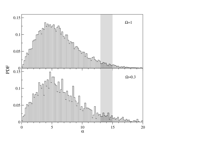
Figure 2: The simulated PDF of the misalignment angle between velocity and smoothed gravity for LG candidates. Upper panel: $\Omega=1.0$; lower: $\Omega=0.3$. Shaded area represents observational constraints from the PSCz catalogue.

The values of the angle we obtained are smaller than the value obtained by Davis et al. (1991) from N-body simulations, $10.2^{\circ}$. However, we use the spectrum of the PSCz galaxies, while the power spectrum they used was a standard CDM. This model has more power on small (nonlinear) scales, so we expect a larger effect in this case. We additionally calculated the angle in a standard CDM model (the power spectrum given by eq. 5 with $\Gamma=0.5$). The mean angle indeed increased from $7.0^{\circ}$ to $8.1^{\circ}$. The rest of the difference we attribute to differencies between the numerical codes (hydro vs. N-body).

4 The relation for amplitudes

In the previous Section we have shown that the misalignment angle between the vectors of velocity and gravitational acceleration is small. Therefore, most information about the relation between the two vectors is contained in the relation between their amplitudes. This is also the crucial point in determining $\Omega$ from the LG dipole. Figure 3 shows this relation for the LG candidates in models with $\Omega=1$ and $\Omega=0.3$. Here, both gravity and velocity fields are smoothed with a top-hat filter of radius $500$ $\hbox{km}\cdot\hbox{s}^{-1}$.

Figure 3: Modules of 500 $\hbox{km}\cdot\hbox{s}^{-1}$ top-hat smoothed velocity and gravity for the LG candidates (scatter plots). Top panel: $\Omega=1$, bottom: $\Omega=0.3$. Solid line represents the linear relation, dashed – mean values of $g^{R}$ and $v^{R}$.

In the top panel of Figure 3, the points agree with the linear prediction (solid line) quite well. The reason of this is twofold. First, the model with $\Omega=1$ has a low normalization, so the velocity and gravity fields are only weakly nonlinear. Second, the velocity $600$ $\hbox{km}\cdot\hbox{s}^{-1}$ is rather typical for an $\Omega=1$ universe, while the velocity–gravity relation deviates more significantly from the linear prediction only in the high-velocity tail (Kudlicki et al. 2000b). Specifically, the r.m.s. value of the velocity of all points in the simulation is $458$ $\hbox{km}\cdot\hbox{s}^{-1}$.

Contrary to the previous case, in the lower panel of Figure 3 the points lie farther off the line. This is not surprising, because the normalization of the model with $\Omega=0.3$ is higher, so the fields are more nonlinear. Moreover, the LG velocity of $600$ $\hbox{km}\cdot\hbox{s}^{-1}$ is less typical for an $\Omega=0.3$ Universe. Higher normalization of the model compensates for this effect only partly. The r.m.s. value of the velocity of all points in this model is $340$ $\hbox{km}\cdot\hbox{s}^{-1}$.

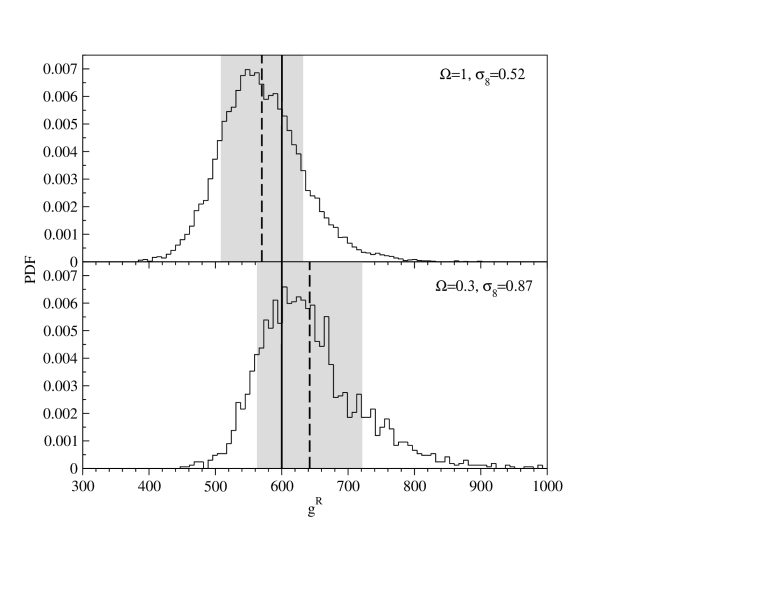
Figure 4: PDF of the smoothed gravity field (histogram). Solid vertical line marks the value of 600 $\hbox{km}\cdot\hbox{s}^{-1}$, dashed – mean values of $g^{R}$ and shaded strips – 1$\sigma$ intervals around the mean values.

The above discussion does not, however, imply that the gravitational acceleration of the LG is a better estimator of the LG velocity in a $\Omega=1.0$ than in a $\Omega=0.3$ Universe. As described earlier, in actual comparisons one uses the smoothed gravity of the LG as an estimator of its unsmoothed velocity. In Figure 3 we see that, for both models, the mean smoothed velocity of the LG candidates (dashed horizontal line) is smaller than their unsmoothed velocity, $v=600$ $\hbox{km}\cdot\hbox{s}^{-1}$. As stated in the previous Section, it means that part of the central velocity has been induced by mass fluctuations within the smoothing radius. Since $\langle v^{R}\rangle<v$, though for the flat model $\langle v^{R}\rangle\simeq\langle g^{R}\rangle$, $\langle g^{R}\rangle$ should be smaller than $v$. Figure 4 show distributions of the values of $g^{R}$. For $\Omega=1$, $\langle g^{R}\rangle=570$ $\hbox{km}\cdot\hbox{s}^{-1}$(dashed vertical line), so indeed $\langle g^{R}\rangle<v$. Thus, the smoothed gravitational acceleration of the LG is in this case a slightly biased estimator of its unsmoothed velocity, and essentially all bias results from estimating unsmoothed velocity by its smoothed counterpart, and not from nonlinear gravity. The difference between $\langle g^{R}\rangle$ and $v$ results in a systematic error of the estimate of $\beta$ of 5.3 %.

As for the model with $\Omega=0.3$, the situation is different. The effects of nonlinear gravity act in the opposite direction than the effects of smoothing and turn out to dominate over them. The mean value of $g^{R}$ is here $642$ $\hbox{km}\cdot\hbox{s}^{-1}$. In other words, in the $\Omega=0.3$ model the smoothed gravitational acceleration of the LG overestimates its unsmoothed velocity. This results in a systematic error of the estimate of $\beta$ of $6.5$ %.

To sum up, smoothed gravity of the LG underestimates its velocity in a high-$\Omega$ Universe, while it overestimates the velocity in a low-$\Omega$ Universe. Thus, there is no common bias, independent of the assumed model, that can be corrected for in the data analysis. Therefore, the results should be either expressed in a model-dependent way or they are a subject to this systematic error. Fortunately, this error is in any case relatively small, of a few per cent.

Thus far, we have left aside the scatter in the velocity–gravity relation. This scatter results in a random error in the estimate of $\beta$ from the LG velocity–gravity comparison. Unlike the systematic error, this error cannot be reduced in any model, because in practice one does not have at his disposal a whole set of the LG observers, but merely one observer (us). Thus, the NE put also an upper limit on the precision of this method of determining $\beta$. The dispersion of the values of $g^{R}$, $\delta g^{R}$, is $62$ and $79$ $\hbox{km}\cdot\hbox{s}^{-1}$, respectively for the models with $\Omega=1$ and $\Omega=0.3$. This implies that the $1\sigma$ random error in the estimate of $\beta$ due to the NE is $12.3$ % and $10.9$ %, respectively.

The summary of systematic and random errors is presented in Table 1.

$\Omega$ $v/\langle g^{R}\rangle-1$ $\delta g^{R}/\langle g^{R}\rangle$ 0.3 -6.5 % 10.9 % 1.0 5.3 % 12.3 %

Table 1: Systematic and random errors in determining $\beta$ from the LG dipole comparisons due to non-linear effects, for two cosmological models.

5 Summary

Using numerical simulations we have studied the relation between the velocity of the Local Group and its gravitational acceleration. This relation underlies both a test for the kinematic origin of the CMB dipole and a method of estimating $\beta$.

First, we have investigated the mean misalignment angle between the two vectors. For the case of $\Omega=1$, we have confirmed the result of Davis et al. (1991), that this angle is small. Actually, the value we have obtained ($\sim 7^{\circ}$) is even smaller than that of Davis et al. ($\sim 10^{\circ}$). We attribute a part of the difference to the different power spectrum we used, namely, that of the PSCz survey. The rest of the difference is likely caused by the differences between the numerical codes (hydro vs. N-body). We have verified that the misalignment angle is fairly insensitive to $\Omega$, in agreement with our theoretical prediction.

The observed misalignment angle is $\sim 14^{\circ}$, close to the upper limit for the $95$ % confidence interval for the simulated angle. Therefore, the NE are unlikely to be responsible for all of the observed misalignment. Other effects must play a role here as well, like, e.g., incomplete sky coverage and/or shot noise.

Next, we have studied the relation between the amplitudes of the LG velocity and gravity vectors. This relation has a scatter, resulting in a $11$–$12$ % random error of the estimate of $\beta$. In the model with $\Omega=1$, the smoothed gravity of the LG turns out to be a biased low estimator of the LG velocity. On the contrary, in the model with $\Omega=0.3$, the estimator is biased high.

Using mock catalogs constructed for different cosmologies, S99 computed the ratio between the reconstructed gravity dipole at the observer’s position and its true N-body velocity. In a ‘numerical analysis’, they subsequently used the average of all ratios as a multiplicative factor which relates the reconstructed gravity of the LG to the true LG velocity. Since biases due to the NE are distinct for different cosmologies (and this is also true for other effects, like, e.g., the effect of finite volume), an attempt to derive a model-independent estimate of $\beta$ is illegitimate. Rather, the results should be expressed explicitly in a model-dependent way. Indeed, the estimates of $\beta$ for models with $\Omega=1$ and with $\Omega=0.3$, obtained by S99 using an alternative, model-dependent maximum-likelihood analysis are clearly different. We conclude that the ‘numerical analysis’ of S99 is formally incorrect.

While in principle important, in practice the discussed biases are small: of the order of a few per cent. With this accuracy, therefore, to the LG velocity–gravity comparisons the linear theory can be applied. Furthermore, the random error of the estimate of $\beta$ due to the nonlinear effects is small compared to the total random error ($\sim$ 40%: S99). We thus conclude that in the LG velocity–gravity comparisons the NE are not the major concern.

Acknowledgements. We thank Michał Różyczka for useful comments. This research has been supported in part by the Polish State Committee for Scientific Research grants No. 2.P03D.014.19 and 2.P03D.017.19. The numerical computations reported here were performed at the Interdisciplinary Centre for Mathematical and Computational Modeling in Warsaw, Poland.

REFERENCES

• Berlind, A.A., Narayanan, V.K., Weinberg, D.H. 2000, Astrophys. J., 537, 537.

• Davis, M., Strauss, M.A., Yahil, A. 1991, Astrophys. J., 372, 394.

• Eke, V.R., Cole, S., Frenk, C.S. 1996, MNRAS, 282, 263.

• Goroff, M. H., Grinstein, B., Rey, S.-J., Wise, M. B. 1986, Astrophys. J., 311, 6.

• Górski, K., Davis, M., Strauss, M.A., White, S.D.M., Yahil, A. 1989, Astrophys. J., 344, 1.

• Juszkiewicz, R., Vittorio, N., Wyse, R.F.G. 1990, Astrophys. J., 349, 408.

• Kudlicki A., Plewa T., Różyczka M. 1996, Acta Astron., 46, 297.

• Kudlicki A., Chodorowski, M. J., Plewa T., Różyczka M. 2000a, MNRAS, 316, 464.

• Kudlicki, A., Chodorowski, M. J., Strauss, M. A., Cieciela̧g, P. 2000b, MNRAS, in press.

• Kudlicki A., Chodorowski, M. J., Plewa T., Różyczka M. 2000c, in preparation.

• Lahav, O., Rees, M.J., Lilje, P.B., Primack, J.R. 1991, MNRAS, 251, 128.

• Lahav, O., Kaiser, N., Hoffman, Y. 1990, Astrophys. J., 352, 448.

• Lineweaver, C. H., Tenorio, L., Smoot, G. F., Keegstra, P., Banday, A. J., Lubin, P. 1996, Astrophys. J. Letters, 470, 38.

• Nusser, A., Colberg, J.M. 1998, MNRAS, 294, 457.

• Paczynski, B., Piran, T. 1990, Astrophys. J., 364, 341.

• Peebles, P.J.E. 1980, Princeton: Princeton University Press.

• Peebles, P.J.E. 1987, Astrophys. J., 317, 576.

• Rowan-Robinson, M. et al.  2000, MNRAS, 314, 375.

• Strauss, M.A., Yahil, A., Davis, M., Huchra, J.P., Fisher, K. 1992, Astrophys. J., 397, 395.

• Schmoldt, I. et al.  1999, MNRAS, 304, 893.

• Scoccimarro, R., Colombi, S., Fry, J. N., Frieman, J.A., Hivon, E., Melott, A. 1998, Astrophys. J., 496, 586.

• Sutherland, W. et al.  1999, MNRAS, 308, 289.