*

Abstract

We describe here an iterative method for jointly estimating the noise power spectrum from a CMB experiment’s time-ordered data, together with the maximum-likelihood map. We test the robustness of this method on simulated Boomerang datasets with realistic noise.

1 Introduction

The map-making problem for CMB anisotropy measurements was first considered in the context of the COBE-DMR mission [7, 13]. It was further extended to quick algorithms for differential measurements [14] taking into account $1/f$ noise [15]. Given the size of the upcoming datasets ($\geq 10^{6}$ pixels for MAP) it is essential that the map-making algorithm remains quick (typically $O(n_{d}\log L_{N})$ where $n_{d}$ is the number of time-samples, and $L_{N}$ the effective noise-filter length). Another related question, which has been pioneered by [5], is how to determine the noise statistical properties from the data itself. We present a map-making method, based on Wright’s fast algorithm, to compute iteratively a minimum variance map together with an estimate of the detector noise power spectrum which is needed to compute unbiased power spectrum estimators of the cosmological signal.

2 Iterative map-making - Application to simulations

2.1 Method

We model the data stream in the following way:

$${{\rm\bf d_{t}}}={{\rm\bf P_{tp}\Delta_{p}}}+{{\rm\bf n_{t}}}$$ (1)

where ${{\rm\bf\Delta_{p}}}$ is a pixelized version of the observed sky (i.e. convolved by the experimental beam), and ${{\rm\bf n_{t}}}$ is the detector noise after primary deconvolution of any filter present in the instrumental chain (e.g. bolometer time constant, read-out filters). We will assume here that the experiment is a total power measurement, i.e. that the pointing matrix ${{\rm\bf P_{tp}}}$ contains only one non-zero element per row. We now want to estimate the minimum variance map from this data, i.e. the map that minimizes $\chi^{2}=({{{\rm\bf d}}}-{{{\rm\bf P}}\Delta})^{\dagger}{{{\rm\bf N}}}^{-1}({{{\rm\bf d}}}-{{{\rm\bf P}}\Delta})$. The solution is given by:

$$\tilde{\Delta}=\left({{{\rm\bf P}}}^{\dagger}{{{\rm\bf N}}}^{-1}{{{\rm\bf P}}}\right)^{-1}{{{\rm\bf P}}}^{\dagger}{{{\rm\bf N}}}^{-1}{{{\rm\bf d}}}$$ (2)

A few remarks are necessary at this point. First, the matrix to be inverted is huge ($n_{pix}\times n_{pix}$) so that an iterative linear solver is needed. Secondly, the noise correlation matrix $N^{-1}_{tt^{\prime}}$ has to be determined from the data itself. To make this tractable we assume that, at least over subsets of the time-stream, the noise is reasonably stationary, so that the multiplication by ${{\rm\bf N}}^{-1}$ becomes a convolution operator, in other words that it is diagonal in Fourier space . We thus implemented the following algorithm:

          for each stationary noise subset • ${{\rm\bf n}}^{(j)}={{\rm\bf d}}-{{\rm\bf P\tilde{\Delta}}}^{(j)}\Rightarrow{{\rm\bf N}}^{(j)-1}=\langle{{\rm\bf nn}}^{\dagger}\rangle^{-1}$ • ${{\rm\bf\tilde{\Delta}}}^{(j+1)}-{{\rm\bf\tilde{\Delta}}}^{(j)}=\left({{\rm\bf P^{\dagger}W^{*}P}}\right)^{-1}{{\rm\bf PN}}^{(j)-1}{{\rm\bf n}}^{(j)}$ endfor

To keep the algorithm as fast as possible, we took ${{\rm\bf W^{*}}}$ to be diagonal and constant, so that ${{\rm\bf P^{\dagger}W^{*}P}}$ is diagonal, with each element being equal to the number of observations per pixel, up to a multiplicative constant. The choice of the numerical value of this constant is only important for the convergence properties of the algorithm. In this form, the algorithm is very similar to a Jacobi iterative solver (in which we would have $\left(diag\{{{\rm\bf P^{\dagger}N}}^{-1}{{\rm\bf P}}\}\right)^{-1}$ instead of $\left({{\rm\bf P^{\dagger}W^{*}P}}\right)^{-1}$). It has the additional advantage of being very easy to compute, for very similar convergence properties. Since we made the assumption that each noise matrix is diagonal in Fourier space, all time-domain operations are done in Fourier space using FFTs, thus reducing the number of floating point operations to $O(L_{N}\log L_{N})$ for each subset.

The advantages of this iterative method are obvious: it is fast ($O(n_{d}\log L_{N})$ operations) and cheap in memory ($O(L_{N})$ storage). However, since we try to estimate both the noise power spectrum and the map in a leap-frog manner, the convergence properties must be studied with numerical simulations. In particular, the stability of the algorithm is function of the number of parameters that we use to describe the noise power spectrum. In other words, we have to assume some regularity in the latter, which translated in practice in fitting the amplitude of the noise in frequency band powers of varying width.

2.2 Simulations

To test the properties of the algorithm, we made simulations of Boomerang LDB time-streams with an sCDM sky, i.e. with precisely the same scanning strategy and a beam smoothing comparable to the 150a channel. We chose this channel because it was used to determine the angular power-spectrum $C_{\ell}$ of the CMB anisotropies [2]. The 10 days of data are approximately divided in two halves corresponding to two different azimuthal scan speeds (2 degrees, then 1 degree per second) at a mean elevation of $\sim 45$ degrees. These two scan-speeds excited differently mechanical/thermal resonances in the instrument payload, and therefore were characterized by different noise power-spectra at low frequency; we simulated the noise time-streams for both halves according to the noise power spectra as measured by our method over the 150a data.

These power spectra are shown in figure 1 (left panel), for both scan velocities. One can see in particular that for the two degree per second spectrum (dotted line) the scan-synchronous harmonics are much stronger than in the one degree per second spectrum (where the scan-synchronous signal is actually dominated by the dipole emission). For a more complete description of these effects, as well as a precise description of the instrument, we refer the reader to Brendan Crill’s thesis ([3]).

The right panel of figure 1 shows the (1 degree per second) spectrum of the simulated (signal+noise) data (magenta) together with the recovered noise spectrum (black). One can see that most of the signal power is concentrated in a smooth continuum contribution between $\sim 0.1\,{\rm Hz}$ and $\sim 3-4\,{\rm Hz}$ (which corresponds approximately to the beam size). This plot shows that a naive estimation of the noise from the data time-stream would typically result in overestimating the noise by $\sim 10\,\%$ at the degree scale.

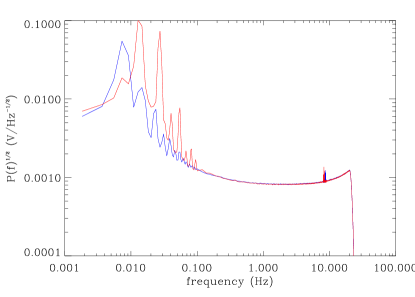
Figure 1: Left panel: Time-stream noise spectra of the two halves of the 150a channel data, estimated with the method described in section2.1. The blue line corresponds to one degree per second data (1 dps), the red line to 2 dps data. Note the difference of amplitude in the scan-synchronous lines. Right panel: Spectrum of the (signal+noise) 1 dps simulated data (magenta) together with the recovered noise power spectrum (black).

In principle, the presence of strong scan-synchronous lines in the noise power spectra at low frequency, as well as the overall $1/{\rm f}$ property of the noise could be taken into account by the method which would down-weight those frequencies accordingly, but in practice, because of the phase-coherent, non-gaussian nature of those scan-synchronous patterns we had to high-pass filter the data at $0.06\times{\rm scan\,speed\,(Hz)}$. This changes the effective pointing matrix ${{\rm\bf P}}$ to ${{\rm\bf FP}}$ where $F$ is the high-pass filter; however, looking at Eq. 2, this is equivalent to leaving ${{\rm\bf P}}$ unchanged, and replacing ${{\rm\bf N}}^{-1}$ by ${{\rm\bf F^{\dagger}N}}^{-1}{{\rm\bf F}}$, which is straightforward in Fourier space.

The Boomerang data set provides a flag with each sample data, indicating the mode of observation (CMB scans, source scans, SZ regions, etc.) and the quality of the data (either good or bad, where bad data corresponds to cosmic ray contamination or a scan elevation change resulting in fluctuations of the cold plate temperature). We thus flagged as bad in our simulations all samples not corresponding to good CMB scan data. In principle, the proper way to deal with such a data with gaps would be to construct the orthonormal noise eigenmodes basis with support constrained to the valid chunks, and do the whole analysis on this basis instead of Fourier space. However, given the length of the time-stream considered here ($\sim 5\times 10^{7}$ time samples) it is completely impractical. The solution we adopted was to model those gaps as being samples spent on the observation of a $0\,{\rm K}$ internal calibrator considered as an additional fake pixel. We had thus to make constrained realizations of the noise time-stream as measured by the algorithm at each iteration step in those gaps, and assign their pointing matrix element outside the map to this fake pixel.

Here again, the length of the time-stream comes again as a problem, since the constrained realizations involve in the best case (when the separation between gaps is bigger than the noise correlation length $N_{\rm cor}$) inverting a matrix of linear size $N_{\rm cor}$, and in the worse case a matrix of linear size comparable to the entire time-stream. Fortunately, fast algorithms have been developed to answer this problem (known as linear prediction). In particular, we implemented a version of Burg’s algorithm (see e.g. [8]) to solve this problem.

Finally, we used HEALpix $7^{\prime}$ pixels [6], resulting in a $138620$ pixel map. The input simulated map (i.e. “before observation”) is shown in figure 2 (upper left panel), together with the corresponding sky coverage (lower left panel). The different “broad bands” in the coverage file correspond to distinct scan periods of the flight at different constant sky elevations, illustrating the compromise between a uniform sky coverage and a constant elevation scanning strategy (to avoid atmospheric gradients). The lower right panel shows the difference between the input map and the map recovered from the time-stream by the iterative method. We can see several important things in this error map, namely:

• The net effect of the high-pass filtering in the time-stream is to kill the largest scales in the map. The fact that the pointing matrix has been effectively changed by the filtering has been properly taken into account by the algorithm (see discussion above).

• There is no apparent residual striping in the error map, although a more precise way to quantify this statement may be necessary to be able to compare this method with alternative map-making algorithms.

• The apparent horizontal features in the error map are related to non-uniform coverage (compare to coverage map in the lower-left panel), and are not caused by residual striping.

Residual striping can be seen in the upper right panel of figure 2, where the difference of the coadded (“naive”) and iterative maps is shown. We can in particular see that the features follow the mean direction of the scan (as expected from striping) and form a non-zero angle to the iso-dec direction.

The method is not free of caveats however. As in any iterative linear solver, the convergence of the solution, decomposed on the (noise) kernel eigenmodes, is a function of the associated eigenvalue. Thus the noisiest pixel modes (usually at large scales since the time-stream is high-pass filtered, either by hand or as part of the algorithm if the noise is higher at low frequency) take (exponentially) more time to converge. The problem scales as the noise matrix condition number, which is a direct function of the noise power spectrum dynamical range and of the scanning strategy. A solution to this problem [4] is a multi-grid version of the present algorithm, exploiting the hierarchical structure of the HEALPix pixelization, and rebinning the time-stream accordingly. [4] have shown that the convergence rate on large scales is then drastically reduced. Another caveat is that the distribution of the noise power spectrum estimation is skewed, leading to a small bias in the noise estimation. This is similar to the “cosmic bias” discussed by [1] in the case of the $C_{\ell}$’s. A possible solution would be to approximate the likelihood distribution of the noise spectrum estimator to correct for this bias. Finally, this method does not deal yet with beam asymmetry, but fast convolution methods [11] are being developed, and will be ultimately integrated, allowing the addition of different channels with different beams to the same map.

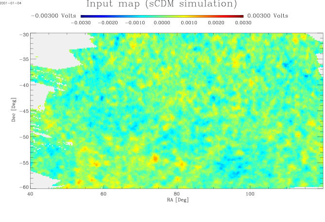
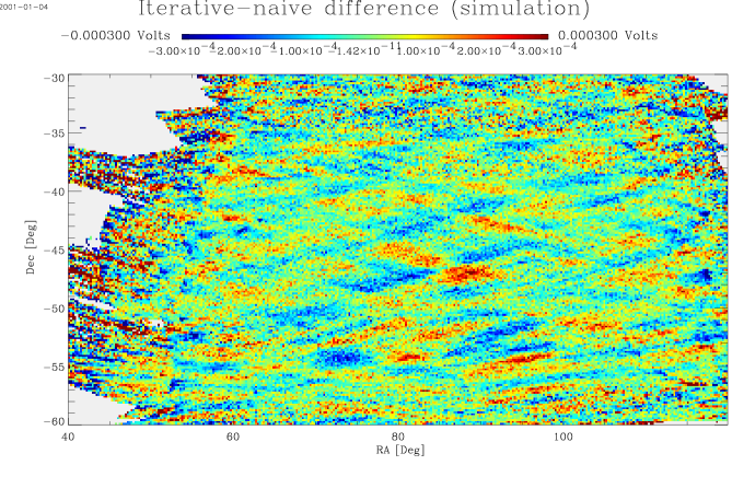
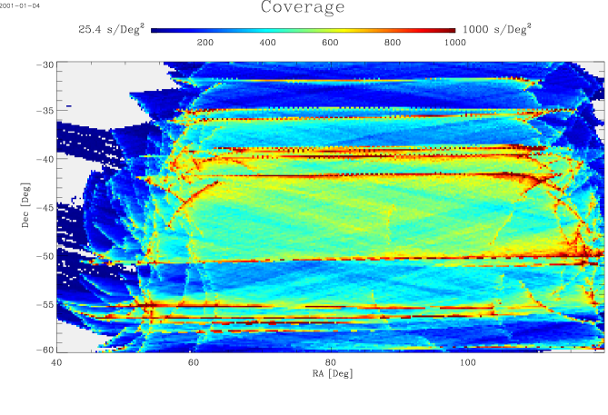
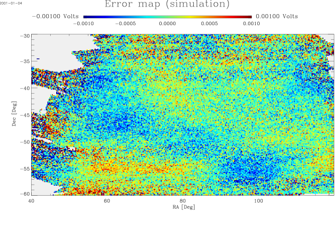
Figure 2: Simulations - Upper left: Input map - Lower left: Coverage - Upper right: Striping map (difference between iterative and coadded map). - Lower right: error map (iterative case). Note the different color scales used for the difference maps.

3 Conclusions - Perspectives

We described a fast iterative map-making method to simultaneously generate the maximum-likelihood map and the noise power spectrum from a scanning experiment time stream. We tested its convergence properties on realistic Boomerang simulations, including the effect of complex scan strategy and noise power spectra, resulting in a complicated noise matrix. We concluded that, except for the spatially largest (and ill conditioned) modes, the map and noise power spectra converge very quickly. This caveat can be cured by means of a “convergence accelerator”, where multi-grid methods provide a very promising solution. In addition, this method, coupled to a fast $C_{\ell}$ quadratic estimator [12, 9], provide a practical way to compute the angular power spectrum of CMB fluctuations in the future megapixel experiments.

References

- [1] J.R. Bond, A.H. Jaffe, L. Knox, Astrophys. Journal 533, 19 (2000)
- [2] P. de Bernardis et al, Nature 404, 955 (2000)
- [3] B.P. Crill, Ph.D. thesis, CalTech. (2000)
- [4] O. Doré, this volume
- [5] P.G. Ferreira & A.H. Jaffe, MNRAS 312, 89 (2000)
- [6] K.M. Górski, E. Hivon, B.D. Wandelt in proceedings of the MPA/ESO Conference, Garching, 2-7 August 1998, eds A.J. Banday, R.K. Sheth and L. Da Costa. See also http://www.tac.dk/ healpix/
- [7] C.H. Lineweaver et al, Astrophys. Journal 436, 452 (1994)
- [8] W.H. Press, B.P. Flannery, S.A. Teukolsky, W.T. Vetterling, 1992, Numerical Recipes, Cambridge University Press
- [9] I. Szapudi, S. Prunet, D. Pogosyan, A. Szalay & J.R. Bond, astro-ph/0010256
- [10] M. Tegmark, Astrophys. Journal Lett. 480, 87 (1997)
- [11] B.D. Wandelt, this volume
- [12] B.D. Wandelt, E. Hivon, K.M. Gorski, astro-ph/0008111
- [13] E.L. Wright, in proceedings of the BCSPIN Puri Winter School
- [14] E.L. Wright, G. Hinshaw, C.L. Bennett, Astrophys. Journal Lett. 458, 53 (1996)
- [15] E.L. Wright, proceeding of the IAS CMB Workshop, astro-ph/9612006