Theory of Extrasolar Giant Planet Transits

Abstract

We present a synthesis of physical effects influencing the observed lightcurve of an extrasolar giant planet (EGP) transiting its host star. The synthesis includes a treatment of Rayleigh scattering, cloud scattering, refraction, and molecular absorption of starlight in the EGP atmosphere. Of these effects, molecular absorption dominates in determining the transit-derived radius $R$, for planetary orbital radii less than a few AU. Using a generic model for the atmosphere of EGP HD209458b, we perform a fit to the best available transit lightcurve data, and infer that this planet has a radius at a pressure of 1 bar, $R_{1}$, equal to 94430 km, with an uncertainty of $\sim 500$ km arising from plausible uncertainties in the atmospheric temperature profile. We predict that $R$ will be a function of wavelength of observation, with a robust prediction of variations of at least $\pm 1$% at infrared wavelengths where H₂O opacity in the high EGP atmosphere dominates.

1 Introduction

Measurements of the diminution of starlight during transit of a planet across the disk of a star provide an almost direct means to detect extrasolar giant planets (EGPs) with orbital inclinations close to $90\arcdeg$. When coupled with measurements of the radial velocity variation of the orbited star during motion about the common barycenter, the mass $M$ of the planet can be measured, and the radius $R$ of the planet can be deduced from the depth of the transit lightcurve.

To date, only one transiting extrasolar planet has been observed: HD209458b (Charbonneau et al., 2000; Henry et al., 2000). A high-quality composite transit lightcurve has been obtained using the STIS spectrograph on the Hubble Space Telescope (HST; Brown et al. 2000), and a model fit to the lightcurve and radial velocity data yields the following results: inclination $i=86.68\pm 0.14\arcdeg$, mass $M$=0.69 $M_{\rm J}$ (where $M_{\rm J}$ is the mass of Jupiter), and radius $R=1.347\pm 0.060R_{\rm J}$ (where $R_{\rm J}$ is the radius of Jupiter). Thus, HD209458b has been confirmed as a genuine hydrogen-rich EGP (Burrows et al., 2000). Spectroscopic radial velocity data for HD209458 give a precise value for the planet’s orbital period, $P$=3.524738 days.

Brown et al. (2000) modeled planet HD209458b as a uniform occulting disk of radius $R$. However, as Seager and Sasselov (2000) first pointed out, the value of $R$ for a real planet will be a function of wavelength, depending on the transmissive properties of the planet’s atmosphere, as well as on other properties of the atmosphere, such as the location of dense cloud layers. In this paper, an unsubscripted $R$ will denote such a wavelength-dependent radius, while subscripted $R$s will denote values of the radius at a fixed level in the planet’s atmosphere. Specifically, for purposes of comparing the inferred values of $R$ and $M$ with theoretical models of EGPs of specified age $t$, one should relate the inferred $R$ to the radius of the planet at a specific fiducial pressure, as is done for Jupiter, where $R_{\rm J}$ is customarily expressed as $R_{\rm J}=71492\pm 4$ km, the equatorial radius at a pressure of 1 bar (Lindal et al., 1981). The purpose of the present paper, then, is to fit the HST lightcurve of Brown et al. (2000) to explicit atmospheric models of HD209458b, in order to derive the EGP’s radius at 1 bar pressure, which we will call $R_{1}$. Along the way, we obtain further predictions of the variation of $R$ with wavelength, over a broader range of wavelengths than in the analysis of Seager and Sasselov (2000). Our model for the atmospheric structure is a generic one, but it differs in some respects from that of Seager and Sasselov (2000).

The transit lightcurve depends on (a) Rayleigh scattering of light from the host star, (b) refraction of the stellar surface brightness distribution, and (c) the slant optical depth $\tau$ through the planet’s atmosphere, as determined by molecular opacity and clouds. All of these effects depend in turn upon the atmospheric pressure ($P$) vs. temperature ($T$) profile, and upon the surface gravity $g$.

In the following, we consider the $P$ vs. $T$ profile, effects (a) through (c), and then present results for the relation of $R$ as a function of wavelength $\lambda$ and the best-fit results for $R_{1}$ for HD209458b.

2 Atmospheric Model

2.1 $P-T$ Profile

Our philosophy in constructing the $P-T$ profile of our baseline model for HD209458b is that this profile should be representative for the planet’s albedo class (either Class IV or V), as defined in Sudarsky, Burrows, and Pinto (2000, SBP). The specifics of this profile are not important as long as the basic molecular composition of the atmosphere is respected and the mapping between pressure and areal mass density is correct for a given gravity. The surface gravity of HD209458b is measured to be close to the Earth’s value. Hence, we used the [T_eff=1270 K/gravity=10³ cm s^-2] model for Class IV EGPs, similar to that found in SBP. (Note that the actual $P-T$ profile will be a function of dynamic processes that redistribute heat from pole to equator and to the night side, processes that are difficult to model [Guillot and Showman 2001].)

Figure 1 shows the nominal $P-T$ profile used in the model (solid heavy line on left side), along with high-temperature and low-temperature versions used to explore the sensitivity of the results to the profile. At $P$ = 1 mbar, the difference between the high-temperature and low-temperature profiles is about 500 K, or about 50 percent of the nominal temperature. As we discuss below, the transit radius of HD209458b is primarily determined by opacity sources in the vicinity of $P$ $\sim 10$ mbar. In §7 we discuss the sensitivity of the transit radius to the alternative temperature profiles.

The right-hand side of Fig. 1 shows adiabatic $P-T$ profiles for various interior models of the planet, to be discussed in §8.

2.2 Clouds and Condensates

We predict the altitude at which clouds of various condensable species form using a code summarized in Burrows et al. (2001) and Marley et al. (1999). Vapor pressure relations for the rocky condensates are from Lunine et al. (1989). Above the altitude at which a given condensate first appears, growth rates for particles and droplets are calculated using analytic expressions (Rossow, 1978). The cloud model assumes that the atmospheric thermal balance at each level is dominated by a modal particle size that is the maximum attainable when growth rates are exceeded by the sedimentation, or rainout rate, of the particles. In convective regions, equating the upwelling (convective) velocity and the sedimentation velocity sets the particle size. The amount of condensate at each altitude within the cloud is given by the vapor pressure at that level multiplied by a “supersaturation factor” usually set to 0.01 by analogy with terrestrial clouds. The particle size and the mass density of the condensate at each level thus determine the number density of particles.

The enstatite cloud layer is potentially the most important for affecting the value of $R$. Scattering and extinction cross sections for this major cloud forming species were obtained for the computed particle sizes by a full Mie theory (SBP). The optical properties of enstatite were taken from Dorschner et al. (1995).

Ackerman and Marley (2001) develop a model of cloud formation that extends the foregoing to include a more realistic rainout prescription. However, as shown in Fig. 2, the major cloud forming species for HD209458b, enstatite, does not contribute opacity in the right altitude range to have a significant effect on the transit profiles. More refractory cloud-forming species, e.g., aluminum silicates, occur deeper in the atmosphere. Less refractory cloud formers such as water and sulfur-bearing species would condense out at higher altitude, but the atmosphere is too warm for these species to occur as clouds. Therefore, for HD209458b, our cloud model is more than adequate. It is possible that very minor cloud forming species that are slightly less refractory than enstatite would put some cloud opacity at modestly higher altitudes, but their smaller abundance relative to enstatite would proportionately diminish their effect. We therefore argue that, for this particular extrasolar planet and those with similar effective temperatures, cloud opacity is not significant in determining the transit radius. Adopting the Ackerman and Marley (2001) prescription would likely result in an even less significant role for the enstatite clouds, since such a model would result in rainout of more condensate and lead to a less optically-thick cloud.

3 Rayleigh Scattering

Rayleigh scattering was treated in an approximate manner. As we demonstrate below, Rayleigh scattering has only a minor effect on the value of $R$, so an approximate treatment is sufficient. The effect of Rayleigh scattering (or any other scattering) is complex, because stellar photons incident on the planet’s atmosphere in a given pencil with incident intensity $I$ are partially removed from the pencil and scattered into different solid angles. Thus, if only conservative Rayleigh scattering were occurring, the limb at $R$ would be defined by the radius at which a high probability of such removal occurs. However, photons are scattered into the beam to the observer as well as removed. Rather than treat the full three-dimensional problem of Rayleigh scattering in a spherically-stratified atmosphere, we replaced the atmosphere with a series of slabs located in a plane containing the center of the planet and orthogonal to the star-observer line. In the following, we will denote the two-dimensional vector separation of a point in this plane from the projected planetary center by r, and the scalar value by $r$. The three-dimensional vector position of an atmospheric point from the planetary center will be denoted by r^′′.

Each slab, located at a two-dimensional radius $r$ from the projected planet center, has a Rayleigh-scattering optical depth $\tau_{\rm R}$ given by

$$\tau_{\rm R}=2\int_{r}^{\infty}r^{\prime\prime}dr^{\prime\prime}\sigma_{\rm R}N(r^{\prime\prime})/\sqrt{r^{\prime\prime 2}-r^{2}},$$ (1)

where $N$ is the number density of molecules in the atmosphere, and $\sigma_{\rm R}$ is the Rayleigh-scattering cross-section per molecule, given by

$$\sigma_{\rm R}={{8\pi^{3}(2+\nu)^{2}\nu^{2}}\over{3\lambda^{4}N^{2}}},$$ (2)

where $\nu$ is the refractivity (refractive index minus 1) of the gas (Chandrasekhar, 1960). Since $\nu\ll 1$ and $\nu\propto N$, $\sigma_{\rm R}$ is a function only of $\lambda$ and the gas composition.

We wrote a Monte Carlo scattering code to investigate the effects of Rayleigh scattering in the planet’s atmosphere. The code follows every photon as it travels through a plane-parallel slab of a given optical thickness. Incident photons can arrive at the top of the slab from any direction on an imaginary hemisphere. Inside the slab, after every scattering event, a new photon direction in three dimensions is calculated, based on the Rayleigh-scattering phase function. Photons are followed until they emerge from either side of the slab, and the total path traveled, in units of optical depth, is tabulated. When the photon finally emerges from the bottom of the slab it is placed into a bin that corresponds to its final direction. Upon completion, the total number of photons in each bin is obtained, along with the average path traveled per photon in that bin.

Our code was tested against the analytical results of van de Hulst (1974) and Chandrasekhar (1960). To within the noise in the Monte Carlo simulations ($\sim 1$%), we were able to match van de Hulst’s results for an isotropic distribution of photons and Chandrasekhar’s for isotropic and “pencil beam” distributions at a variety of incident angles.

We ran our simulations for radiation at normal incidence to the slab for a variety of different optical thicknesses, logarithmically spaced from 0.01 to 28. If we assume an imaginary observer looks at normal incidence from the other side of the slab, the observer will see photons that pass through the slab unobstructed, as well as those that are multiply scattered back into the beam and emerge normal to the surface. Of most interest to us in this situation are those photons that, although scattered, emerge normal to the slab surface and ultimately reach the observer. These photons create a Rayleigh-scattering “glow” from the slab. We found that the glow intensity in the direction of the observer increases until $\tau_{\rm R}\sim 3.4$, as fewer and fewer photons are able to pass through the slab unscattered. At $\tau_{\rm R}>3.4$, up to $\tau_{\rm R}=28$, the greatest thickness we ran, Rayleigh-scattered intensity decreases more or less exponentially, as a larger fraction of the photons are scattered back out the top of the slab, rather than scattering all the way through. We fitted an equation to both sides of this curve so that the glow intensity could be interpolated, and extrapolated to higher $\tau_{\rm R}$ if necessary. We also fitted an equation to the average optical path length traveled for these photons, using this result to estimate the total molecular-absorption optical depth, $\tau_{\rm M}$, and cloud optical depth, $\tau_{\rm C}$. The total optical depth for photons initially incident with impact parameter r is then given by $\tau=\tau_{\rm R}+\tau_{\rm M}$+$\tau_{\rm C}$. In practice, for all cases that we have investigated, $\tau_{\rm M}$ becomes large long before $\tau_{\rm R}$ or $\tau_{\rm C}$ does. Likewise, refractive effects are still negligible when $\tau_{\rm M}$ becomes significant, as discussed below. Thus, for purposes of computing $\tau_{\rm M}$, the photon path can be taken to be a straight line through the planetary atmosphere, such that

$$\tau_{\rm M}=2\int_{r}^{\infty}r^{\prime\prime}dr^{\prime\prime}\sigma_{\rm M}N(r^{\prime\prime})/\sqrt{r^{\prime\prime 2}-r^{2}},$$ (3)

where $\sigma_{\rm M}$ is the average absorption cross-section per molecule for a solar-composition planetary atmosphere. We estimate $\tau_{\rm C}$ with a similar formula, although strictly speaking, it becomes appreciable at levels where refraction is important.

Since in our transit calculations the planet is a disk passing in front of its star, we assume the atmosphere of the planet is a flat slab with an optical thickness that decreases with increasing distance from the planet center. In this way, our results for different slab thicknesses can be used directly in our planetary atmosphere calculations.

In our transit simulations, the atmosphere of the planet was broken up into many small annuli, each with its own optical thickness, which is dependent on wavelength, as calculated using our model for the structure of the planet’s atmosphere. At a given wavelength of light, for every optical thickness in the atmosphere, the Rayleigh glow intensity was calculated. This intensity results in a small additive component to the star plus planet signal outside of transit, but in general has no detectable effect on the observed light curve. In addition, since the total average path traveled for a scattered photon is also known, the effects of absorption due to molecular opacity can be calculated. At high optical thicknesses, most scattered photons that would emerge from the slab are actually absorbed by opacity sources in the atmosphere.

4 Refraction

The theory used to compute refractive effects is essentially identical to that of the standard theory for occultations of stars by planetary atmospheres (Hubbard, Yelle, and Lunine, 1990). In the following, we let $I({\bf r})$ denote the photon intensity within a differential solid angle whose coordinates are labeled by the two-dimensional vector r measured in the plane of the sky, from the center of the planet. The intensity $I({\bf r})$ of the observed image of star plus planet is then given by the mapping

$$I({\bf r})=I^{\prime}({\bf r^{\prime}})e^{-\tau(r)},$$ (4)

where $I^{\prime}({\bf r^{\prime}})$ is the stellar surface brightness distribution, $\tau$ is the total optical depth integrated along a ray path with impact parameter $r$, and ${\bf r^{\prime}}$ and r are two-dimensional vectors in a plane normal to the propagation direction, marking the starting point of a ray on the stellar surface and its closest-approach position in the planet’s atmosphere, respectively.

The mapping from ${\bf r^{\prime}}$ to r is obtained by computing the total phase shift $\Phi$ imposed by the refractivity distribution on a photon with impact parameter $r$,

$$\Phi(r)=(4\pi/\lambda)\int_{r}^{\infty}r^{\prime\prime}dr^{\prime\prime}\nu(r^{\prime\prime})/\sqrt{r^{\prime\prime 2}-r^{2}},$$ (5)

then computing the two-dimensional bending angle ${\boldsymbol{\alpha}}$ according to ${\boldsymbol{\alpha}}=(\lambda/2\pi)\nabla\Phi$, where the gradient is taken in the two-dimensional plane.

Figure 2 shows the calculated values of $\tau_{\rm M}$, $\tau_{\rm R}$, and cloud optical depth, $\tau_{\rm C}$, for our best-fit planetary model, as discussed in §6. Figure 2 also shows the atmospheric radius where refraction begins to be important. Specifically, the shaded region in Fig. 2 shows the difference between $r$ and $r^{\prime}$ at a level where the difference,

$$r-r^{\prime}=D\alpha,$$ (6)

becomes equal to 500 km, or about one atmospheric scale height ($D$ is the distance from the star to the planet). The upper edge of the shaded region corresponds to $r$ and the lower edge to $r^{\prime}$. Since $\alpha$ varies exponentially with $-r$, considerable ray bending occurs for impact parameters below the shaded region. However, $\tau_{\rm M}$ is always so large in this region that refraction is unimportant for defining $R$, for values of $D$ similar to that of HD209458b.

We do not include general-relativistic ray bending in the theory presented in this paper, as it is unimportant for the parameters of HD209458b. However, it is straightforward to include gravitational lensing. One simply adds to the refractive $\alpha$ discussed above, an additional term for general-relativistic ray bending, $\alpha_{\rm GR}=4GM/rc^{2}$ (where $G$ is the gravitational constant, $M$ is the planet’s mass, and $c$ is the speed of light). The total bending angle used in Eq. (6) is then $\alpha+\alpha_{\rm GR}$.

5 Gaseous Opacities

The primary gaseous absorptive opacity sources in the atmospheres of hot EGPs include H₂, H₂O, CH₄, CO, and the important alkali metals, Na and K. We take the temperature- and pressure-dependent opacities from theoretical and experimental data referenced in Burrows et al. (1997) and Burrows et al. (2001). In the near infrared ($\sim$1 to 2.6 $\mu$m), absorption by H₂O molecules figures most prominently, with strong ro-vibrational bands centered at $\sim$0.95, 1.15, 1.4, 1.85, and 2.6 $\mu$m. The strong pressure-broadened resonance lines of neutral Na and K – the strengths of which depend on the level of ionization by stellar irradiation – appear prominently at $\sim$0.59 and 0.77 $\mu$m, respectively. The dominant carbon-bearing molecule is a function of both temperature and pressure. At lower temperatures, CH₄ is dominant, but CO overtakes CH₄ at higher temperatures ($\sim$950 K at 0.1 bar, $\sim$1100 K at 1 bar). Hence, the strengths of CH₄ features (1.4, 1.7, 2.2 $\mu$m) and CO features (1.2, 1.6, 2.3 $\mu$m) are highly temperature-dependent. Finally, an important continuous opacity source in cloud-free EGPs is H₂-H₂ collision induced absorption at high pressures and temperatures (Zheng and Borysow, 1995).

All of the opacity sources mentioned above were used to calculate $\sigma_{\rm M}$, and then incorporated in Eq. (3); the results are plotted in Fig. 2.

6 Transit Lightcurve

The next step in calculating a transit lightcurve was to synthesize images of the two-dimensional distribution of starlight around the planet. We created a synthetic square aperture of size $361\times 361$ pixels (1 pixel = spatial scale of 700 km), centered on the planet. The star was taken to be a disk with a pixel intensity of $1$ at its center, with a prescribed darkening law to the limb. At each pixel in the array, the pixel intensity was calculated using the calculated values of the various $\tau$s, adding the Rayleigh-scattered component into the beam and the refracted stellar component, from each pixel on the stellar disk (including contributions from virtual pixels on the part of the stellar profile outside the synthetic aperture). The total pixel sum over the aperture was then calculated, with and without the planet present, allowing us to calculate the total intensity subtracted and added by the planet.

We then synthesized a transit lightcurve, incorporating all the physical effects described above, and using most of the fitted parameters of Brown et al. (2000): $i$, stellar radius, and orbital radius and period. The lightcurve was obtained by averaging over the bandpass of the Brown et al. (2000) experiment, weighted by a blackbody distribution for the effective temperature of HD209458. The value of $R_{1}$ for HD209458b was adjusted in our model until we matched the depth of the theoretical transit lightcurve to the depth of the composite observed lightcurve, as shown in Fig. 3. The match of our model, which has only the adjustable parameter $R_{1}$, to the data is quite good. We obtain $R_{1}=94430$ km for HD209458b, for the nominal $P-T$ profile shown in Fig. 1. For the cold profile, we obtain $R_{1}=95000$ km, and for the hot profile, $R_{1}=94260$ km.

The flux from the star was computed using limb-darkening coefficients from Van Hamme (1993). The two equations used were the nonlinear logarithmic and square-root laws. These laws are (logarithmic):

$$I(\mu)/I(1)=1-A(1-\mu)-B\mu\ln(\mu),$$ (7)

and (square root):

$$I(\mu)/I(1)=1-C(1-\mu)-D(1-\sqrt{\mu}),$$ (8)

where $I(1)$ is the specific intensity at the center of the stellar disk, $A$, $B$, $C$, and $D$ are wavelength-dependent constants, and $\mu$ is the cosine of the angle between the line of sight and the emergent intensity.

The curve shown in Fig. 3 is for the logarithmic law; we found that use of the square root law instead changed the lightcurve by less than 1 part in 400. The coefficients used were interpolated from the Van Hamme monochromatic coefficient tables, for $\log g=4.3$, $T_{\rm eff}$ of 6000 K, and solar metallicity. The very slight mismatch with the data is perhaps due to a difference in the calculated stellar intensities, which are based on the stellar models of Kurucz (1991), and the actual change in stellar intensity across the disk.

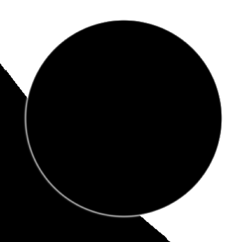
Figure 4: (a) Synthetic image of a transit of HD209458b (pixel scale is from 0 to 1, with 1 corresponding to the intensity at the center of the stellar disk), with the planet at an orbital position $5\arcdeg$ from inferior conjunction, at a wavelength of 0.45 $\mu$m. Close scrutiny will show a faint Rayleigh-scattering ring around the planet’s limb exterior to the stellar limb. (b) An image of the same geometry, but with molecular opacity reduced by a factor 1000, and with the pixel scale stretched over the range 0 to 0.1. The Rayleigh-scattering ring is thus wider and brighter.

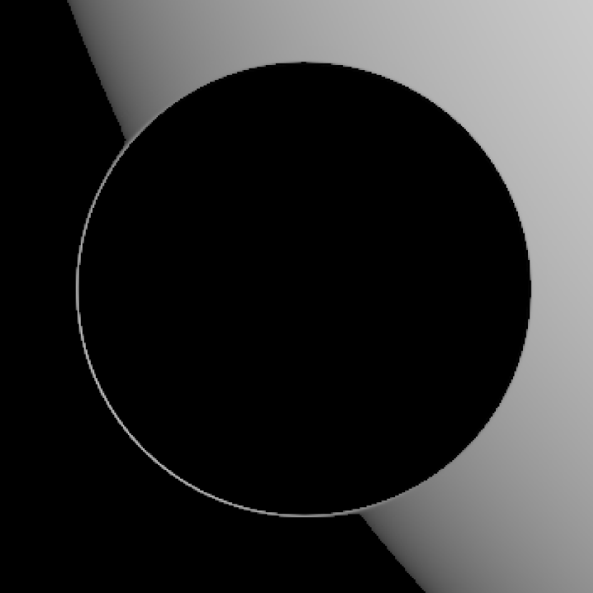
Figure 5: Image of the same atmosphere as in Fig. 4(a) (pixel scale is again from 0 to 1), but with the distance $D$ from the planet to the star increased from the value for HD209458b to a value $10^{4}$ times greater. The bright limb outlining the planet’s disk is far brighter than the Rayleigh “glow”, and is produced by refractive mapping of the stellar disk’s intensity distribution.

Figures 4 and 5 show examples of synthetic images and provide more details about the contributions of Rayleigh scattering and refraction to the shape of a transit lightcurve, which are generally negligible for the specific case of HD209458b. In Fig. 4a, we show that even at a short wavelength of 0.45 $\mu$m, the forward-scattered Rayleigh glow is almost invisible. In Fig. 4b, we reduce $\tau_{\rm M}$ by a factor $10^{3}$ and stretch the image to make the narrow Rayleigh glow annulus more apparent.

In Fig. 5, we retain the atmospheric structure for the nominal model corresponding to Fig. 4(a), but we increase the distance $D$ to $10^{4}$ times the value for HD209458b, thus bringing the refracting layers of the atmosphere into play. According to Eq. (6), for $r-r^{\prime}$ fixed at, say, one scale height ($\sim 500$ km), then if $D$ increases by $10^{4}$, $\alpha$ must decrease by the same factor. Since $\alpha$ is roughly proportional to pressure in the atmospheres considered here, a decrease in $\alpha$ by this factor corresponds to displacing the layer responsible for the prescribed refraction upward by about nine scale heights, to a region where the slant optical depth $\tau$ is negligible. The atmospheric depth where the limb of bright refracted starlight terminates is determined by the abrupt increase of $\tau$ to appreciable values.

As $D$ increases further, our theory smoothly transforms to conventional ray-optical stellar occultation theory in the limit $\tau=0$ (Hubbard, Yelle, and Lunine, 1990), appropriate to observation of the passage of a planet in front of a star of smaller apparent angular size than the planet.

Except for such conventional stellar occultations, we are unlikely to observe a transit dominated by refractive effects, as the probability of a transit by an EGP at an orbital radius of hundreds of AU is exceedingly small.

7 Variation of $R$ with $\lambda$

As discussed above, the relation $R(\lambda)$ is almost entirely determined by molecular absorption features. Seager and Sasselov (2000) discussed a possible dramatic variation of $R(\lambda)$ due to alkali absorption features in the visual wavelength bands. We predict dramatic effects at infrared wavelengths as well, due to strong features of H₂O; however, detection of infrared variations in $R(\lambda)$ may require observations above the Earth’s atmosphere.

Figure 6 shows, for HD209458b parameters, the $R(\lambda)$ relation predicted by our three $P-T$ models. This relation is computed by evaluating binned averages of opacities (for specified temperatures) at 500 individual frequencies spaced across several $\times 10^{4}$ original frequencies. Note that the variation of $R$ vs. $\lambda$ increases with $T$ at some wavelengths, and decreases at others. Note also that though a flattened temperature gradient in the upper atmosphere will smooth out the reflection/emission spectrum of the planet itself, the variation $R(\lambda)$ with wavelength will not be similarly flattened. For example, even though the Na/K alkali metal features in the planet’s spectrum may be smoothed by stellar irradiation, the transit size will still vary appreciably across these features as long as Na/K are not ionized.

Because the variations with wavelength are quite rapid in some wavelength intervals, it may be possible to strategically choose wavelengths of observations which will span these rapid variations and still be close enough together to allow the limb-darkening of HD209458 to be removed by fitting a smooth model. Note that $R$ is typically about 2000 km larger than $R_{1}$, and thus pertains to atmospheric layers which are at pressures near $\sim 10$ mbar.

8 Conclusions

Referring back to Fig. 1, note that an adiabat in a solar-composition object with a mass of 0.69 $M_{\rm J}$, which would yield a value of $R_{1}$ compatible with the one determined here, must have a significantly lower specific entropy than the atmospheric layers heated by the star. It follows that there must be a significant region in the planet, possibly spanning pressures from $\sim 10$ to $\sim 10^{4}$ bar, where the $T$ vs. $P$ relation must be substantially subadiabatic or even isothermal. Detailed thermal evolution models for this layer remain to be calculated.

We have shown that apparent variations of at least $\pm 1$% in the radius of giant planets occur as a function of wavelength. This variation is potentially discernable with the next generation of transit-observing spacecraft in Earth orbit, provided that they possess the capability of multi-wavelength observation with sufficient spectral resolution. We therefore recommend that proposers or designers of such missions consider the possibility of transit-based probing of extra-solar planet atmospheric composition, via multi-wavelength observations.

Finally, as is suggested by Fig. 6, there could be considerable variation in $R(\lambda)$ at ultraviolet wavelengths. Indeed, as is well known (Smith and Hunten, 1990), the location of the level where $\tau\sim 1$ in our own giant planets is a strong function of ultraviolet wavelength, and in the UV is typically at much lower pressures than 1 $\mu$bar. Observation of an EGP transit at UV wavelengths is, in many experimental aspects, equivalent to a solar-occultation UV experiment in our solar system, and may have similar diagnostic power for chemical composition of the high planetary atmosphere. To be sure, Jupiter has a rather warm stratosphere/mesosphere, with photochemical aerosols, so the UV radius could be a sensitive function of the external boundary conditions within which an EGP planet finds itself.

Figure 1: Heavy line on the left shows the nominal atmospheric pressure-temperature profile used in these calculations; light solid line shows the low-temperature version and open-dotted line shows the high-temperature version. Dashed lines show interior H-He adiabats, with the corresponding entropy (in units of Boltzmann’s constant per baryon) and total radius $R_{1}$ for a planet mass of 0.69 $M_{\rm J}$. Heavy dashed line shows the approximate interior adiabat that matches the transit-derived value of $R_{1}$.

Figure 2: Radius vs. optical depth for $\tau_{\rm M}$ (dashed), $\tau_{\rm R}$ (dotted), and $\tau_{\rm C}$ (dot-dashed), for the nominal $P-T$ profile and for parameters of HD209458b. Below the shaded zone near 1 bar pressure, refraction is also significant. Molecular opacity profiles are plotted for wavelengths spanned by the observations of Brown et al. (2000).

Figure 3: Synthetic transit lightcurve for our model (solid curve), compared with composite lightcurve of Brown et al. (2000). The three $P-T$ profiles give indistinguishable solid curves.

Figure 6: Predicted variation of transit radius $R$ with wavelength (heavy curve, nominal $P-T$ profile; light curve, cold $P-T$ profile; open dots, hot $P-T$ profile; see Fig. 1). The right-hand scales show, in percent, the variation of $R$ with respect to $R_{1}$ and with respect to $R_{\rm T}$, an $\sim$“average” transit radius in the visual wavelength band, adopted as $R_{\rm T}=96500$ km $=1.35R_{\rm J}$. At wavelengths where slant optical depth is high, $R$ is larger. “Absorption” features thus appear upside-down on this plot. Prominent features are labeled with the responsible molecule.