Attractors and Isocurvature Perturbations in Quintessence Models

Abstract

We investigate the evolution of cosmological perturbations in scenarios with a quintessence scalar field, both analytically and numerically. In the tracking regime for quintessence, we find the long wavelength solutions for the perturbations of the quintessence field. We discuss the possibility of isocurvature modes generated by the quintessence sector and their impact on observations.

I Introduction

Observational data seems to indicate that we live in an accelerating Universe [1]. As an alternative to the scenario where the acceleration is fueled by a cosmological constant $\Lambda$, models with a scalar field capable of dominating recently and of developing a negative pressure have been proposed [2]. This scalar field which pervades our universe has been dubbed quintessence.

Compared to the cosmological constant, quintessence has two important differences. First, quintessence can be interpreted as a fluid with a time dependent equation of state. Therefore quintessence models may alleviate the so-called coincidence problem, which is the apparent cosmic collusion that the dark energy component is fine-tuned in a way that it is starting to dominate the energy density of the universe just at the present time. And second, in contrast to the cosmological constant, the quintessence field can fluctuate [2, 3, 4, 5, 6, 7].

One interesting possibility is that the quintessence field $Q(\vec{x},t)$ can, in combination with the other cosmic fluids (radiation, baryons, cold dark matter, etc.), lead not only to adiabatic (curvature) perturbations, but to a mixture which includes an isocurvature component. Isocurvature (or entropy) perturbations appear when the relative energy density and pressure perturbations of the different fluid species combine to leave the overall curvature perturbations unchanged. In quintessence models, the presence of potentially relevant isocurvature modes could be generic, just as in multi-field inflationary models [8]. Indeed, quintessence is constructed is such a way that it is an unthermalized component subdominant for most of the history of the Universe. Since quintessence is uncoupled from the rest of matter because of astrophysical and cosmological constraints [9], its fluctuations may lead to an isocurvature component, whose nature will be preserved except for the known integrated feeding of the adiabatic component, expressed by the relation [10, 11]:

$$\dot{\zeta}=\frac{2}{3H(1+w)}\left[c_{s}^{2}\frac{\nabla^{2}\Phi}{a^{2}}+\frac{1}{2}\delta p_{\rm nad}\right]\;,$$ (1)

where $\zeta$ is the gauge-invariant curvature perturbation, a dot denotes time derivative, $w\equiv p/\rho$ and $c_{s}^{2}\equiv\dot{p}/\dot{\rho}$ denote respectively the equation of state and the speed of sound of the total matter content, $p_{\rm nad}$ is the total non-adiabatic pressure perturbation and we employ units such that $8\pi G=1$.

This latter effect was studied [12] in the context of axion perturbations, and [13] in the context of the baryon isocurvature model [14]. This effect is also responsible for the growth of super-Hubble adiabatic perturbations during preheating [15]. Considering axions as Cold Dark Matter (CDM) [12], an isocurvature perturbation due to the angle misalignment produced during inflation induces an adiabatic component of comparable amplitude at the moment of reentry of the perturbation inside the Hubble radius. This is due to the fact that the CDM component is going to dominate about the time of decoupling, and thus the integrated effect is almost completed by the time that mode reenters inside the Hubble radius.

However, the quintessence case is different from the axion/CDM since in most of the models quintessence fluctuations are damped inside the Hubble radius. This is required in order to minimize the impact of an additional dynamical degree of freedom on structure formation. The quintessence and the axion/CDM differ also in either one of two ways: i) Q was still a negligible component before the time of decoupling, or ii) Q was comparable to normal matter, $\Omega_{Q}={\cal{O}}(1)$, but in a so-called tracking regime [4, 16] whereby its equation of state $w_{Q}\equiv p_{Q}/\rho_{Q}$ was approximately that of dust or radiation — whichever was dominating at the time. In the first case (which happens, for example, in the PNGB scenario [17]) isocurvature perturbations are irrelevant simply because the field $Q(\vec{x},t)$ is a negligible component until a redshift of at least $z\sim 10$. In the second case the energy density in $Q$ need not be small, however due to the tracking of the quintessence field, perturbations in the $Q$-fluid behaved similarly to the perturbations in the background for most of the observable history of the Universe, and isocurvature perturbations are therefore suppressed until the end of the tracking phase. In either case, a primordial isocurvature perturbation could still be present, but it would not have had enough time to induce an adiabatic component.

From an observational point of view, isocurvature perturbations have a very distinctive imprint on the spectrum of the temperature anisotropy of the Cosmic Microwave Background (CMB) [18, 19, 20]. With the accuracy that future CMB experiments such as MAP [21] and Planck [22] will be able to reach, the constraints on the ratio of uncorrelated isocurvature perturbations in CDM-radiation to the adiabatic component will be of the order of percents [23, 24]. Recently the impact of generic isocurvature modes on the estimation of cosmological parameters has been also investigated [25]. Therefore it is important to understand the evolution of isocurvature modes in quintessence models where an unthermalized, uncoupled relic survives until the present era, and dominates very recently. In most of the literature a primordial adiabatic spectrum for quintessence perturbations is assumed. If the notion of adiabaticity among different components is related to their thermal equilibrium, then the weakly coupled nature of quintessence could evade this condition. The primordial spectrum could be generated during inflation and/or influenced through its evolution until the decoupling time.

The outline of the paper is as follows. In section II we give necessary notions of the background evolution of quintessence models. In section III we study the evolution of cosmological perturbations and we identify the attractor solution for quintessence perturbations during the tracking regime. In section IV we study the evolution of isocurvature perturbations and their feedback on the adiabatic component. In section V we discuss the initial condition for quintessence perturbations after nucleosynthesys. We conclude in section VI.

II Background evolution with quintessence

For simplicity we consider only radiation, pressureless matter and quintessence, and ignore the neutrinos as well as the distinction between baryons and CDM. Each component $i$ ($i=r,m,Q$) has an energy density $\rho_{i}$ and pressure $p_{i}$. The sum of the energy densities determines the Hubble parameter via the usual Einstein equation, $3H^{2}=\rho=\sum_{i}\rho_{i}$. The equation of state $w_{i}\equiv p_{i}/\rho_{i}$ is $1/3$ and zero in the case of radiation and matter, respectively. The background energy density and the pressure of the quintessence field are:

$$\rho_{Q}=\frac{1}{2}\dot{Q}^{2}+V(Q)\quad,\quad p_{Q}=\frac{1}{2}\dot{Q}^{2}-V(Q)\;,$$ (2)

where the background scalar field $Q(t)$ obeys the equation $\ddot{Q}+3H\dot{Q}+V_{,Q}=0$. This means that $w_{Q}$ is in general time-dependent.

The main requirement of quintessence is that it starts to dominate the energy density of the Universe only at the present time, with an equation of state $w_{Q}(z=0)\equiv w_{Q0}<0$. Conservative phenomenology dictates that $\rho_{Q0}/\rho_{0}=\Omega_{Q0}<0.8$ — to allow time for galaxy formation — and that $w_{Q0}<-0.5$ — to accommodate the SNIa data [26]. In addition, nucleosynthesis demands that $\Omega_{Q}<0.2$ at $z\simeq 10^{9}$.

Model building should obtain these values and still manage to solve (or at least alleviate) the coincidence problem without too much fine tuning (see, e.g., [27].) The main problem seems to be that in order to solve the coincidence problem one needs a period of tracking, but it is hard to get a period of tracking and still obtain $w_{Q0}<-0.5$. It is certainly possible to construct potentials which implement both conditions [7], however we prefer to look at simpler potentials which contain features which are generic to most of the models. As it turns out, the relevant features of the cosmological perturbations do not depend on the specific form of the potential, but only on its generic phenomenology.

In a typical scenario, nicely reviewed in [7], the scalar field starts out subdominant deep in the radiation era, in a kinetic phase with an equation of state $w_{Q}=+1$ (see Fig. 1.) The kinetic energy $\frac{1}{2}\dot{Q}^{2}$ eventually decays, leaving only the quintessence potential energy, which is nearly constant and as a result $w_{Q}\rightarrow-1$ (of course, the quintessence field could also start already in the potential-energy dominated regime). This is the so called potential phase. When $\Omega_{Q}$ becomes of order unity, the quintessence field undergoes a transition which puts it into a tracking regime, where it follows approximately the equation of state of the background. Finally, at some point late in the matter era $Q$ starts to dominate and the Universe begins the accelerated expansion phase that we observe today (the Q-dominated phase.)

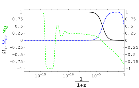
FIG. 1.: Densities of radiation (solid line, black) and matter (dotted line, blue), and the equation of state for the scalar field (dashed line, green), as a function of redshift for a model with potential $V(Q)=M^{4}e^{f/Q}$. In this plot $M^{4}=10^{-70}M_{pl}^{4}$ and $f=1\,M_{pl}$ (with $8\pi G=M_{pl}^{-2}$.)

As long as we keep away from the time of equal matter and radiation ($z_{eq}\simeq 10^{4}$ in our flat models with $H_{0}=65$ Km s^-1 Mpc^-1), one of the two barotropic fluids (radiation or matter) can be neglected. The equation of state of the total matter content then reads:

$$w\equiv\frac{p}{\rho}=w_{F}+(w_{Q}-w_{F})\Omega_{Q}\;,$$ (3)

where the subscript $F$ stands for either radiation, when $t\ll t_{eq}$, or matter, when $t\gg t_{eq}$. The total speed of sound $c_{s}^{2}$ has a simple expression as well:

$$c_{s}^{2}\equiv\frac{\dot{p}}{\dot{\rho}}=w_{F}+\frac{\dot{Q}^{2}}{\rho+p}(c_{Q}^{2}-w_{F})\;,$$ (4)

where $c_{Q}^{2}\equiv\dot{p}_{Q}/\dot{\rho}_{Q}$. It is useful to note that

$$c_{Q}^{2}=1+\frac{2V_{,Q}}{3H\dot{Q}}=w_{Q}-\frac{\dot{w}_{Q}}{3H(1+w_{Q})}\;.$$ (5)

When $c_{Q}^{2}=$constant, then $\dot{Q}\propto V_{,Q}/H$. Taking the time derivative of $c_{Q}^{2}$ we also obtain:

$$\frac{2V_{,QQ}}{3H^{2}}=\frac{1}{H}\frac{d}{dt}c_{Q}^{2}+(c_{Q}^{2}-1)\left[1+\frac{\dot{H}}{H^{2}}-\frac{1}{2}\left(3c_{Q}^{2}+5\right)\right]\;.$$ (6)

When $w_{Q}$ is approximately constant, then from Eq. (5) $c_{Q}^{2}$ is constant as well. By using the background relation $\dot{H}/H^{2}\simeq-3(1+w_{F})/2$ we obtain

$$V_{,QQ}\simeq\frac{9}{4}H^{2}(1-c_{Q}^{2})(w_{F}+c_{Q}^{2}+2)\equiv\alpha H^{2}\;.$$ (7)

We observe that quintessence fluctuations are effectively massless ($V_{QQ}\simeq 0$) during the kinetic phase ($c_{Q}^{2}=1$) and the potential phase ($c_{Q}^{2}=-2-w_{F}$ [7]).

A good quantity to measure how closely the quintessence field $Q$ tracks the background is the quantity $\gamma\equiv V_{,QQ}V/(V^{2}_{,Q})$ — which was named $\Gamma$ in [2]. When $w_{Q}$ is approximately constant in time, then:

$$\gamma\simeq 1+\frac{w_{F}-w_{Q}}{2(1+w_{Q})}\,.$$ (8)

If tracking is exact (as is the case in the exponential potential models), $w_{F}=w_{Q}$, then $\gamma=1$ and $V_{,QQ}/V_{,Q}=V_{,Q}/V$.

If $w_{Q}$ is approximately constant, then the kinetic and potential energies of the scalar field $Q$ must be proportional to each other. Taking the time derivative of $\rho_{Q}\propto\dot{Q}^{2}\propto V$ we obtain that during a tracking phase:

$$\frac{V_{,Q}}{V}=-3(1+w_{Q})\frac{H}{\dot{Q}}\simeq{\rm constant}\;,$$ (9)

where we have used the fact that $\dot{Q}^{2}\propto a^{-3(1+w_{Q})}$ to find $H/\dot{Q}\propto a^{-3(w_{F}-w_{Q})}\propto$ constant, if $w_{Q}\simeq w_{F}$.

We note that during the phases in which $w_{Q}$ is constant $\Omega_{Q}$ goes as:

$$\Omega_{Q}\equiv\frac{\rho_{Q}}{\rho_{\rm TOT}}=a^{3(w_{\rm TOT}-w_{Q})}\,.$$ (10)

Therefore in the radiation epoch $\Omega_{Q}$ redshifts as $a^{-2}$ during its kinetic phase, and it grows as $a^{4}$ during its potential phase. During the tracking regime $\Omega_{Q}$ is approximately constant (depending on how accurate is the tracking) and in the Q-dominated regime it is evidently constant (since $\Omega_{Q}\rightarrow{\cal O}(1)$ when $Q$ dominates.)

III Evolution of perturbations

We compute the evolution of the cosmological perturbations in longitudinal (or conformal-Newtonian) gauge [10]:

$$ds^{2}=(1+2\Phi)dt^{2}-a^{2}(t)(1-2\Phi)d{\bf x}^{2}\;.$$ (11)

In the matter sector, the perturbed energy density and pressure of quintessence are, as usual,

$$\delta\rho_{Q} = \dot{Q}\delta\dot{Q}-\dot{Q}^{2}\Phi+V_{,Q}\delta Q\;,$$ (12)

$$\delta p_{Q} = \dot{Q}\delta\dot{Q}-\dot{Q}^{2}\Phi-V_{,Q}\delta Q\;,$$ (13)

where the Fourier transforms of the scalar field fluctuations obeys the equation:

$$\delta\ddot{Q}+3H\delta\dot{Q}+\frac{k^{2}}{a^{2}}\delta Q+V_{,QQ}\delta Q=+4\dot{Q}\dot{\Phi}-2V_{,Q}\Phi\;.$$ (14)

The density fluctuations in radiation and matter, on the other hand, obey the conservation equations for the density contrasts $\delta_{F}\equiv\delta\rho_{F}/\rho_{F}$:

$$\dot{\delta}_{F}-3(1+w_{F})\dot{\Phi}=(1+w_{F})\frac{k}{a(t)}V_{F}\;,$$ (15)

where $V_{F}$ is the fluid velocity. In the long wavelength limit ($k\ll aH$) this equation is extremely useful, since it reads:

$$\delta_{F}-3(1+w_{F})\Phi={\rm constant}=\delta_{F}^{i}-3(1+w_{F})\Phi^{i}\;,$$ (16)

where the superscript $i$ indicates that the fluctuations have been evaluated at some initial time $t_{i}$. We can also combine Eq. (15) for $\delta_{F}$ with the equation for conservation of momentum,

$$\dot{V}_{F}=-\frac{k}{a(t)}\left(\frac{w_{F}}{1+w_{F}}\delta_{F}+\Phi\right)\;,$$ (17)

and obtain a simple second order equation for $\delta_{F}$:

$$\delta_{F}\,^{\prime\prime}+w_{F}k^{2}\delta_{F}=3(1+w_{f})\left(\Phi\,^{\prime\prime}-\frac{k^{2}}{3}\Phi\right)\;,$$ (18)

where a prime denotes, as usual, derivative with respect to conformal time $\eta$, where $d/d\eta\equiv a(t)d/dt$.

We consider now the evolution of the quintessence field perturbations. At first, let us neglect the metric perturbations, i.e. take Eq. (14) without its right-hand side. By using the rescaled variables $\delta\tilde{Q}=a^{1/2}\delta Q$, Eq. (14) can be rewritten as:

$$\delta\tilde{Q}^{\prime\prime}+{\cal H}\delta\tilde{Q}^{\prime}+\left[k^{2}+a^{2}V_{,QQ}-\frac{a^{\prime\prime}}{2a}-\frac{{\cal H}^{2}}{4}\right]\delta\tilde{Q}=0\;,$$ (19)

where ${\cal{H}}=a^{\prime}/a=aH$.

In a radiation dominated universe $a\propto\eta$ and the term proportional to the second time derivative of the scale factor vanishes; when Eq. (7) holds, then the solutions for the field perturbations in rigid space-times are:

$$\delta Q\sim\eta^{-1/2}\times\left\{\begin{array}[]{c}J_{|\nu|}(k\eta)\\ J_{-|\nu|}(k\eta)\end{array}\right.\;,$$

where

$$\nu^{2}=\frac{1}{4}-\alpha\,.$$ (20)

If $\alpha\neq 0$ both the solutions decay in time. If $\alpha\rightarrow 0$ then there is a constant mode.

The argument above holds for a matter dominated universe as well: if $\alpha=0$ there is a constant mode, otherwise both the solutions decay in time (for a matter dominated universe the appropriate rescaled variable is $\delta\tilde{Q}=a^{3/4}\delta Q$.)

The inclusion of gravitational fluctuations in Eq. (14) leads to a constant solution for the quintessence perturbations in the long-wavelength limit. From Eq. (14) we immediately see that in this limit there are constant solutions $\Phi(t)\rightarrow\Phi^{c}$ and $\delta Q(t)\rightarrow\delta Q^{c}$:

$$\delta Q^{c}\simeq-2\frac{V_{,Q}}{V_{,QQ}}\Phi^{c}\;,$$ (21)

as long as $V_{,Q}/V_{,QQ}$ is approximately constant. But this is precisely what happens during the tracking regime: from Eqs. (9) and (8) we see that $V_{,Q}/V_{,QQ}\simeq V/V_{,Q}\simeq$ constant in the tracking period. We stress that the type of solution (21) does not hold in the kinetic and potential phases, since in these cases $V_{,QQ}\rightarrow 0$.

We can use the $0-0$ component of the Einstein equations to relate the Newtonian potential to the energy densities of other fluids

$$-6H^{2}\Phi-6H\dot{\Phi}-2\frac{k^{2}}{a^{2}}\Phi=\delta\rho_{r}+\delta\rho_{m}+\delta\rho_{Q}\;.$$ (22)

In the long wavelength limit, assuming that $\Phi$ is stationary and ignoring the subdominant barotropic fluid we obtain:

$$-2\Phi\simeq\Omega_{F}\delta_{F}+\Omega_{Q}\delta_{Q}\;.$$ (23)

In the regime described by the attractor in Eq. (21) the perturbed energy density for quintessence, defined in Eq. (12), reduces to:

$$\delta\rho_{Q}^{c} \simeq -2\left(1-\frac{V_{,Q}V_{,QQQ}}{V_{,QQ}^{2}}\right)\dot{Q}^{2}\Phi^{c}-2\Phi^{c}(\frac{\dot{Q}^{2}}{2}+\frac{V}{\gamma})$$ (24)

$$\simeq -2\,\Phi^{c}\left[\rho_{Q}-(\dot{Q}^{2}+V)\frac{\gamma-1}{\gamma}+{\cal O}(\dot{\gamma})\right]\;.$$ (25)

and the perturbed pressure defined in Eq. (13) is:

$$\delta p_{Q}=-2\,p_{Q}\,\Phi+2\Phi(\dot{Q}^{2}-V)\frac{\gamma-1}{\gamma}+{\cal O}(\dot{\gamma})\;.$$ (26)

Using now the background identities $3H^{2}=\rho$ and $\Omega_{Q}\simeq 1-\Omega_{F}$ into Eq. (25), we obtain the density contrasts as functions of the Newtonian potential in the tracking regime:

$$\delta_{Q}^{c}\simeq\delta_{F}^{c}\simeq-2\Phi^{c}\;.$$ (27)

Notice that during tracking, quintessence and the dominant fluid species are in effect indistinguishable ($\delta_{Q}^{c}\simeq\delta_{F}^{c}$), consequently we expect isocurvature perturbations to be suppressed during that period.

A solution corresponding to (21) — though in the synchronous gauge — was first obtained in the case of exponential potentials, for which tracking is exact [4]. An attractor for quintessence perturbations has also been conjectured in [7]. As we have shown, the approximate solutions (21) and (27) hold for any potential, just as long as there is tracking, and, of course, they exist in any gauge.

We can also combine Eqs. (27) and (16) to obtain a relationship between the initial and final values of the Newtonian potential:

$$\Phi^{c}\simeq-\frac{1}{6}\left(\delta_{r}^{i}-4\Phi^{i}\right)\;,$$ (28)

where $\delta_{r}^{i}$ and $\Phi^{i}$ are initial conditions for the radiation density contrast and the Newtonian potential respectively. Notice that these initial conditions can be specified even at a time when quintessence is dominating, and even if the radiation contrast and the Newtonian potential are initially not constant.

We have numerically verified formulas (21), (25), (27) and (28) for several scenarios and initial conditions. Take for example the scenario whose background appeared in our Fig. 1. Two typical initial conditions for the field perturbations are plotted in Figs. 2A and 2B (solid and dashed lines), together with the attractor solutions (thin red lines): as the scalar field starts to approach the tracking regime at $z\simeq 10^{12}$, the perturbations start to converge around the attractor solution. As seen in Fig. 2A for the field perturbations $\delta Q$, the attractor of Eq. (21) is a very good approximation even after the tracking phase has ended — that is, Eq. (21) is a very good approximation during the quintessence-domination period as well, even though $\delta Q$ is not constant anymore. Fig. 2B shows how the quintessence density contrasts converge to $-2\Phi$. In fact, for a wide range of initial values the scalar field perturbations end up at the same solution $\delta Q^{c}$ after tracking.

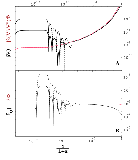
FIG. 2.: Quintessence field fluctuations $\delta Q$ (panel A) and quintessence energy density contrasts $\delta_{Q}$ (panel B) for two different initial conditions for $\delta Q$ and $\delta\dot{Q}$ (solid and dashed lines.) We have chosen initial conditions such that $\Phi\simeq 10^{-5}$ at $z_{\rm dec}=10^{3}$. In panel A the quintessence fluctuations (dashed and solid black lines) are compared with the attractor $-2\Phi V_{,Q}/V_{,QQ}$ (thin red line). Notice that even after the tracking phase ends the analytic approximation of Eq. (21) remains very good. In panel B the quintessence energy density contrasts (solid and dashed black lines) are compared with $-2\Phi$ (thin red line), verifying the second approximation, Eq. (27). The approximation becomes worse as the tracking ends. In both plots the wavelengths of the modes cross the Hubble radius at $z=0$.

This can be also seen in Fig. 3, which is the phase diagram for the perturbations with different initial conditions shown in Fig. 2. During tracking the solutions spiral down to the attractor (solid and dashed lines.) When tracking ends the attractor disappears, but by that time most modes have settled down to the same value, and their evolution is henceforth the same (see the thin red line in Fig. 3 which springs from the attractor point.) We note that this attractor occurs generally only during tracking and for long wavelengths: when the wavelength becomes important (of the order of the inverse effective mass ), there is a sensitivity with respect to the initial conditions of the quintessence perturbations.

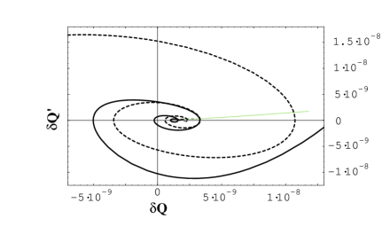
FIG. 3.: Phase diagram for quintessence fluctuations with two different initial conditions. The attractor point $(-2\Phi V_{,Q}/V_{,QQ},0)$ is a transient attractor, valid only for long wavelength modes. As soon as the tracking regime of the field $Q$ terminates, the attractor disappears and the field perturbations start to evolve (green straight line.) However, by the time tracking is over, most long-wavelength solutions have already converged to the same value, and thereafter their evolution is almost indistinguishable.

Summarizing the results of this section: in the kinetic and potential phases there is a constant long wavelength solution which is a linear combination of the initial field fluctuations and of the gravitational potential, as one can see from the initial evolution in Fig. 2A. In the tracking period the quintessence perturbation stabilizes at the attractor solution (21) and it remains at that constant value until the perturbation reenters the Hubble radius, or until quintessence starts to dominate the background.

IV Evolution of isocurvature perturbations

Cosmological fluctuations are often characterized in terms of the gauge-invariant curvature perturbation on comoving hypersurfaces, defined as [10]:

$$\zeta\equiv\frac{2}{3}\frac{\dot{\Phi}/H+\Phi}{1+w}+\Phi\;.$$ (29)

The time variation of the intrinsic curvature $\zeta$ is given, on large scales, by the non-adiabatic pressure or, equivalently, by the amplitude of the isocurvature perturbations — see Eq. (1). Therefore, if the non-adiabatic pressure vanishes then $\zeta$ is constant.

The pressure perturbations can be split into adiabatic and non-adiabatic components:

$$\delta p=\left.\frac{\delta p}{\delta\rho}\right|_{\delta\Gamma=0}\delta\rho+\left.\frac{\delta p}{\delta\Gamma}\right|_{\delta\rho=0}\delta\Gamma\;,$$ (30)

where we define the entropy perturbation $\delta\Gamma$ as [28]:

$$\delta\Gamma\equiv\frac{\delta p}{\dot{p}}-\frac{\delta\rho}{\dot{\rho}}\;.$$ (31)

As a consequence we have that the adiabatic pressure perturbation is given by

$$\delta p_{\rm ad}=c_{s}^{2}\delta\rho\equiv\left.\frac{\delta p}{\delta\rho}\right|_{\delta\Gamma=0}\delta\rho=\frac{\dot{p}}{\dot{\rho}}\delta\rho\;,$$ (32)

and the non-adiabatic pressure is given by the second term in the right-hand side of the definition (30):

$$\delta p_{\rm nad} = \left.\frac{\delta p}{\delta\Gamma}\right|_{\delta\rho=0}\delta\Gamma=\dot{p}\,\delta\Gamma$$ (33)

$$= \delta p-c_{s}^{2}\delta\rho\equiv\sum_{i}\left(\delta p_{i}-c_{s}^{2}\delta\rho_{i}\right)\;.$$ (34)

We now give an analytic description of the time evolution of isocurvature perturbations for long wavelengths. We work perturbatively assuming $\zeta$ constant, and compute the non adiabatic pressure $\dot{p}\,\delta\Gamma$: when the integrated effect is large, it means that isocurvature perturbations cannot be neglected. The results of this analysis confirm the methods of the previous section (where $\Phi$ was assumed constant) and are in agreement with the numerical analysis.

Using Eq. (33) we find that the non-adiabatic pressure is given by:

$$\delta p_{\rm nad}=\left(w_{r}-c_{s}^{2}\right)\delta\rho_{r}+\delta p_{Q}-c_{s}^{2}\delta\rho_{Q}\;,$$ (35)

By using Eqs. (3) and (4) into Eqs. (35) one can check that in general

$$\frac{\delta p_{\rm nad}}{\rho+p}={\cal O}(\Omega_{Q})\times(\delta_{r}+\delta_{Q})\;.$$ (36)

Therefore, when the quintessence contribution to the total energy density is very subdominant, the isocurvature contribution is small. However, since the isocurvature contribution to $\zeta$ is an integrated effect, $\dot{\zeta}\sim t\delta p_{\rm nad}$, we should study the time evolution of each term which enters into the definition of the non-adiabatic pressure (35).

The first term in the right-hand side of Eq. (35) is proportional to $\rho_{r}\delta_{r}$ and leads at most to a logarithmic increase of $\zeta$.

Among the contributions from the pressure and the energy density of the scalar field we neglect the first term in the right-hand sides of both Eqs. (12) and (13). The term $\dot{Q}^{2}\Phi$ is suppressed during the kinetic phase, but leads to a growth as $a^{7+3w_{\rm TOT}}$ in the left-hand-side of Eq. (36) in the potential regime. During the tracking regime $\dot{Q}^{2}$ gives approximately a constant contribution to (36). The term $V,_{Q}\delta Q$ depends explicitly on the quintessence fluctuations: it decays during the kinetic phase and it grows less rapidly than $\dot{Q}^{2}\Phi$ during the potential regime. However, it leads to a growth as $a^{3/2(1+w_{\rm TOT})}$ during the tracking regime.

It is clear from Eq. (33) that for two barotropic fluids with the same equation of state and the same density contrast the non-adiabatic pressure should be zero. Therefore for exact tracking, quintessence and radiation equilibrate to give zero non-adiabatic pressure. We can also compute the non-adiabatic pressure in the tracking regime by using Eqs. (35), (4) and (8):

$$\delta p_{\rm nad} \simeq \frac{\dot{Q}^{2}}{\rho+p}(w_{r}-c_{Q}^{2})\left(\rho_{r}\delta_{r}-2\Phi\rho_{Q}\right)$$ (38)

$$+{\cal O}[(\gamma-1)\rho_{Q}\Phi]$$

As expected, the non-adiabatic pressure vanishes for exact tracking ($\gamma=1$), otherwise it is small, but not vanishing, during tracking. In general $\delta p_{\rm nad}$ is proportional to $\rho_{Q}$, therefore small in many models.

There is however still one possibility that allows for significant isocurvature fluctuations from quintessence: this happens when the tracking phase starts only at a relatively late redshift, $z\sim 10^{5}-10^{3}$ (see also the next Section, Figs. 4, 5 and 6.) During the transition from the potential phase to the tracking phase, we can have both $\Omega_{Q}$ non-negligible, and the equation of state and speed of sound of quintessence differ substantially from those of the background fluid. If the quintessence density contrast is of the same order of the matter density contrast at decoupling time $z_{\rm dec}\sim 10^{3}$, the isocurvature perturbations can leave an imprint on the CMBR. Later, as tracking forces the field perturbations to the attractor, the isocurvature fluctuations are temporarily depressed, at least until $Q$ starts to dominate at $z\sim 0$.

V Initial conditions: adiabatic or mixed?

In this section we address the issue of how initial conditions of quintessence perturbations can be used as tools in CMBFAST [30]. These initial conditions are set after nucleosynthesis, at $z\sim 10^{9}$. In most of the literature, the initial conditions for the quintessence fluctuations are set up by requiring adiabaticity with the other components [5]. However, the notion of a purely adiabatic perturbation (as well for a purely isocurvature one) is an instantaneous notion for a multifluid system. Moreover, because of the unthermalized nature of quintessence, the adiabatic condition for this component is even less justified.

The adiabatic condition[5, 6] is usually defined as the vanishing of the relative entropy and its time derivative:

$${S}_{rQ} = 0\;,$$ (39)

$$\dot{S}_{rQ} = 0\;,$$ (40)

which reduces, in longitudinal gauge, to:

$$\delta Q = \dot{Q}^{2}\left(V,_{Q}-\frac{k^{2}}{a^{2}}\frac{\dot{Q}}{6H}\right)^{-1}\left(-\frac{\delta_{r}V,_{Q}}{4H\dot{Q}}+\frac{kV_{r}}{6aH}\right)\;,$$ (41)

$$\delta\dot{Q} = \dot{Q}^{2}\left(V,_{Q}-\frac{k^{2}}{a^{2}}\frac{\dot{Q}}{6H}\right)^{-1}\left[-\frac{k^{2}}{6a^{2}H}\left(\frac{3}{4}\delta_{r}+\Phi\right)\right.$$ (43)

$$\left.+V,_{Q}\left(\Phi-\frac{\ddot{Q}\delta_{r}}{4H\dot{Q}}-\frac{kV_{r}}{6aH}\right)\right]\;.$$

The relative entropy between the radiation and the quintessence components is defined as:

$$S_{rQ}\equiv\frac{\delta_{r}}{1+w_{r}}-\frac{\delta_{Q}}{1+w_{Q}}\,.$$ (44)

From the above relation we immediately understand that $S_{rQ}=0$ in the case of exact tracking. Indeed, two fluids with the same equation of state and the same density contrast are undistinguishable. For long wavelengths relations (41)-(43) reduce to:

$$\delta Q \simeq -\frac{\dot{Q}}{4H}\delta_{r}\simeq\frac{\dot{Q}}{2H}\Phi$$ (45)

$${\delta\dot{Q}} \simeq \dot{Q}\left[\Phi+\frac{\delta_{r}}{4}\left(3+\frac{V,_{Q}}{H\dot{Q}}\right)\right]$$ (46)

$$\simeq -\frac{\dot{Q}}{2}\,\Phi\left(1+\frac{V,_{Q}}{H\dot{Q}}\right)$$ (47)

where the second line of Eq. (47) holds only if radiation is the dominant component.

The conditions (45)-(47) should be compared with the solutions during the kinetic and potential phases, $\delta Q=$constant and ${\delta\dot{Q}}=0$, or with the attractor solution Eq. (21) which applies during the tracking phase:

$$\delta Q \simeq -2\frac{V,_{Q}}{V,_{QQ}}\Phi$$ (48)

$${\delta\dot{Q}} \simeq -2\dot{Q}\,\Phi\left(1-\frac{V_{,Q}V_{,QQQ}}{V^{2}_{,QQ}}\right)\;.$$ (49)

It is not hard to see from Eq. (49) that in the tracking regime $\delta\dot{Q}\rightarrow 0$, since $V_{,Q}/V_{,QQ}\simeq V_{,QQ}/V_{,QQQ}$. Using this fact together with Eq. (9), we also obtain that Eqs. (45) and (48) are similar during the tracking regime. Therefore, as expected, if the scalar field is tracking normal matter, then the adiabatic condition is approximately satisfied.

We illustrate the previous discussion in Figs. 4, 5 and 6. The background model is plotted in Fig. 4, and in Figs. 5-6 we present possible scenarios for the perturbations, as well as a comparison with the cosmological perturbations in the $\Lambda$CDM case.

The upper (thin red) curves of Fig. 5 plot the gauge-invariant curvature $\zeta$, defined in Eq. (29). The lower (black) curves are the Newtonian potential $\Phi$. All plots in Fig. 5 have been normalized so that $\Phi=5.10^{-6}$ at $z=10^{9}$, and the wavelengths corresponds to modes which are crossing the Hubble radius at the present time ($z=0$.)

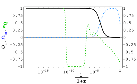
FIG. 4.: Background evolution in a quintessence scenario with the Ratra-Peebles potential $V(Q)=M^{4+\alpha}Q^{-\alpha}$, where $\alpha=6$ and $M=10^{-6.15}$. Plotted are the densities of radiation (solid line, black) and matter (dotted line, blue), and the equation of state for the scalar field (dashed line, green), as a function of redshift.

The solid lines of Fig. 5 correspond to the cosmological perturbations of a fiducial $\Lambda$CDM scenario with adiabatic initial conditions. Notice that, as usual, since $\zeta$ remains constant, $\Phi$ has to change by $9/10$ after $z_{eq}=10^{4}$.

The long-dashed lines of Fig. 5 are the perturbations in a scenario (ICDM) where, in addition to the adiabatic mode, CDM and radiation have an initial relative isocurvature of $S_{rCDM}=3\Phi/2$.

The short-dashed lines are the perturbations in the case of adiabatic initial conditions (AIC) between all components at $z\sim 10^{9}$. The dotted lines are the perturbations in the case where we choose zero isocurvature between radiation and CDM, and $\delta Q=10^{-3}$, $\delta\dot{Q}=0$ initially (QIC.) This last set of initial conditions (QIC) is motivated by the fact that the field perturbations are constant during the kinetic and the potential phases — see, e.g., Fig. 2A.

Notice the identical late isocurvature effect in AIC and QIC. The signal of this effect is the extra growth of the Bardeen parameter $\zeta$ at late times (compare the dotted and short-dashed lines with the solid line in the interval $0<z<10$ in Fig. 5.) This effect is independent from the initial conditions for the quintessence fluctuations. In fact, as already emphasized, the notion of adiabaticity (as well as pure isocurvature) is an instantaneous one, imposed at an initial time, and it does not persist in a multi-fluid system. We stress that this effect is distinct from the change of the Newtonian potential $\Phi$ which is due to the late change in the equation of state of the background, which can be seen in pure form in the $\Lambda$CDM case (solid line in Fig. 5.) A similar change in $\Phi$ occurs also at $z_{\rm eq}=10^{4}$, while $\zeta$ remains constant across the transition between radiation- and matter-domination.

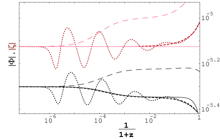
FIG. 5.: Newtonian potential (lower, black curves) and gauge-invariant curvature $\zeta$ (upper, red curves), normalized by the condition that $\Phi=5.10^{-6}$ at $z=10^{9}$. The solid lines are a fiducial $\Lambda$CDM model. The remaining lines correspond to different initial conditions for the fluctuations of the radiation, matter and quintessence components. The long-dashed lines correspond to the case where there is no isocurvature component between $Q$ and radiation, but there is an initial isocurvature component between radiation and CDM. The short-dashed line corresponds to the case of pure adiabatic initial conditions (AIC). The dotted lines correspond to the case of $\delta Q=10^{-3}$, $\delta\dot{Q}=0$ initially (QIC). All modes cross the Hubble radius at $z=0$.

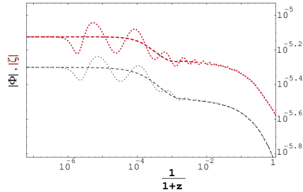
FIG. 6.: Newtonian potential (lower, black curves) and gauge-invariant curvature $\zeta$ (upper, red curves), for a wavelength which crosses the Hubble radius at decoupling time between matter and radiation. The normalizations and the initial conditions are the same of Fig. 5. As in Fig. 5, the short-dashed lines correspond to the case of pure adiabatic initial conditions and the dotted lines correspond to the case of $\delta Q=10^{-3}$, $\delta\dot{Q}=0$ initially. Even for smaller scales, the effect of an isocurvature component is a transient effect. For wavelengths larger than the Hubble radius, the attractor was responsible for explaining the transiency, while for smaller scales the explanation is the decay of quintessence fluctuations inside the Hubble radius.

Notice also the early isocurvature effect in the QIC case (oscillations of the dotted lines in Fig. 5.) This means that there is a substantial non-adiabatic pressure, and hence a large isocurvature perturbation, in this scenario. As we discussed at the end of the previous Section, the reason why isocurvature fluctuations can become important is that the “tracking regime” of the background model only starts relatively late, at $z\sim 10^{5}$. But the quintessence field perturbations need some time to converge to the attractor solution. During this time $\Omega_{Q}$ becomes non-negligible, and since the $Q$ component still behaves quite differently from the dominant background fluid, there can be substantial isocurvature perturbations for wavelengths which cross the Hubble radius at $z\sim 0$. A similar transient effect occurs also for smaller scales, as shown in Fig. 6, for a wavelength which crosses the Hubble radius at the decoupling time. An isocurvature component from the quintessence field leads only to a transient effect, since quintessence fluctuations converge to an attractor for long wavelengths, and decay in time inside the Hubble radius. However, this early transient isocurvature effect can leave an imprint in the spectrum of the CMBR anisotropies.

VI Discussion and Conclusions

We have studied the evolution of cosmological perturbations in quintessence models, with particular attention paid to isocurvature modes generated by quintessence. We have shown that these isocurvature modes are generic, with the exception of the case in which quintessence mimics exactly radiation. This occurs in the tracking phase of models with exponential potentials [4]. However, these models are unappealing from the phenomenological point of view because their equation of state for quintessence is not negative at the present time.

When tracking is not exact, then isocurvature modes are non-vanishing. We found an attractor solution for long wavelength quintessence fluctuations in the tracking regime. This allows an estimation of the amount of isocurvature fluctuations in the tracking regime for any quintessence model that display a tracking period. In the other phases which usually occur in models with quintessence — the kinetic and potential phases — the quintessence fluctuations have also a constant mode, whose actual value is determined by the previous evolution (including inflation.) The contribution of isocurvature fluctuation to the adiabatic mode grows during the potential, tracking and $Q$-domination phases.

We have discussed the assumption of adiabaticity in the context of the setting of initial conditions used in numerical codes such as CMBFAST. As already emphasized, because of the lack of thermal equilibrium, this assumption is not justified for quintessence. However, in the tracking case, the conditions set by the attractor solution are in most cases quantitatively indistinguishable from the adiabatic conditions. Indeed, tracking seems a gravitational mechanism — alternative to thermal equilibrium — which tends to reduce isocurvature modes between quintessence and the background fluid. For models with a tracking phase which starts early in time, we expect a weak dependence on the initial conditions for the quintessence fluctuations. In the stages prior to the tracking phase the “initial conditions” (understood as the values of the field perturbation and its time derivative at a redshift of $z\sim 10^{9}$) depend on the conditions set by inflation, and could be different from the adiabatic ones.

We have identified a late isocurvature effect for long wavelengths due to quintessence. Of course, this is due to the fact that Q dominates at late times, and it is qualitatively independent from the model considered. Therefore, the theoretical explanation of the long wavelength evolution of the Newtonian potential in Q models is a superposition of two effects: the change of the equation of state and the growth of $\zeta$ on super-Hubble scales. This late isocurvature effect could be useful in order to distinguish a cosmological constant model from the models with a quintessence component.

The observational relevance of isocurvature modes generated by quintessence is weakened by the decay in time of quintessence perturbations inside the Hubble radius. For this reason the isocurvature mode in the Q-radiation sector are very different from those in CDM-radiation. This effect was also very appealing in order to minimize the effects of the inclusion of this extra component on structure formation. In the models examined here, the suppression of $\Omega_{Q}$ during the kinetic phase play also a crucial role in order to weaken the effect of some initial isocurvature modes generated by quintessence. Even if the upper bound during nucleosynthesis for $\Omega_{Q}$ is $\sim 0.2$ , the kinetic regime suppresses $\Omega_{Q}$ down to $10^{-15}-10^{-20}$ in the models which we have analyzed. Therefore our considerations may be more relevant for models in which $\Omega_{Q}$ is closer to the upper limit, as, for instance, in the models with a modified exponential potential [31].

It is therefore interesting to study the impact of isocurvature fluctuations in quintessence models using numerical tools such as CMBFAST [30] in which quintessence perturbations are included. In particular, it is possible to construct models where $\Omega_{Q}$ is not so suppressed or in which there is a late tracking phase, in which case isocurvature modes generated by quintessence could lead to observable effects in the temperature anisotropies of the cosmic background radiation.

Acknowledgments

We would like to thank C. Baccigalupi, R. Brandenberger, V. Mukhanov and N. Turok for comments. R. A. thanks the Physics Department at Purdue University for its hospitality at the time of writing the first draft of this paper. F. F. also thanks the Ludwig Maximilians Universität for its hospitality during the final stages of this work. This work was supported in part by the U.S. Department of Energy under Grant DE-FG02-91ER40681 (Task B), and by the Sonderforschungsbereich 375-95 für Astro-Teilchenphysik der Deutschen Forschungsgemeinschaft.

VII Appendix A

Here we present the equations that were evolved numerically. Combining the $0-0$ and $i-i$ Einstein field equations we can eliminate the radiation perturbations, and obtain the following equation for the quintessence and matter perturbations (as explained in the text, we work with units such that $8\pi G=1$, and we have ignored the distinction between baryons and CDM):

$$3\ddot{\Phi} + 15H\dot{\Phi}+\left(12H^{2}+\frac{k^{2}}{a^{2}}\right)\Phi$$ (51)

$$=-\frac{1}{2}\delta_{m}\rho_{m}+\dot{Q}\delta\dot{Q}-\dot{Q}^{2}\Phi-2V_{,Q}\delta Q\;.$$

The equation of motion for the scalar field perturbations is given in Eq. (14). The matter density contrast obeys the energy conservation equation:

$$\dot{\delta}_{m}-3\dot{\Phi}-\frac{k}{a}v_{m}=0\;,$$ (52)

where $v_{m}$ is the matter fluid velocity, which itself satisfies the momentum conservation equation:

$$\dot{v}_{m}+Hv_{m}+\frac{k}{a}\Phi=0\;.$$ (53)

VIII Appendix B

Here we present the evolution of pure isocurvature modes generated by the quintessence sector. Consider contributions from quintessence and another component $X$ to the metric perturbation, which cause a vanishing contribution to $\Phi$ and $\dot{\Phi}$ [10] at some fixed initial time in the energy and momentum constraint. This requires that:

$$\Omega_{Q}\delta_{Q}=-\Omega_{X}\delta_{X}$$ (54)

$$\dot{Q}\delta Q=-\frac{4}{3}v_{X}\rho_{X}\,,$$ (55)

which identifies an isocurvature density mode (54) and an isocurvature velocity mode (55) [19]. The third component $Y$ is the only one which leads to a curvature perturbation (for long wavelengths $-2\Phi=\Gamma_{Y}\delta_{Y}$, as follows from Eq. (23).) The components $X$ and $Y$ are related by adiabaticity ($S_{XY}=0$.) Therefore, the quintessence density contrast at fixed initial time is:

$$\delta_{Q}=-\delta_{X}\frac{\Omega_{X}}{\Omega_{Q}}=2\Phi\left(\frac{1+w_{X}}{1+w_{Y}}\right)\frac{\Omega_{X}}{\Omega_{Y}\Omega_{Q}}$$ (56)

In Fig. 7 the evolution of the Bardeen parameter $\zeta$ for initial pure Q-CDM ($X={\rm CDM}$, solid line) and Q-radiation ($X={\rm radiation}$, dashed line) isocurvature initial conditions at $z=10^{9}$ for the model of Fig. 4. At the initial time the Newtonian potential is so small in order to ensure $\delta_{Q}\leq 1$. However, in both cases - but in particular for the Q-radiation isocurvature initial conditions -, Eqs. (54)-(55) force Q fluctuations to very large values, either initially and in the subsequent evolution. The evolution of Q fluctuations for these type of initial conditions is not described by the attractor (21) – i.e. the inhomogeneous solution to the differential equation for the quintessence fluctuations –, but by the homogeneous solution to Eq. (14). Indeed, in Fig. 7 the growth of the Bardeen parameter saturates roughly when tracking starts in Fig. 4, i.e. when the homogeneous solution for quintessence fluctuations start to decay, as described by Eqs. (19)-(20) with $\alpha\neq 0$.

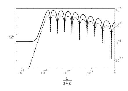
FIG. 7.: Gauge-invariant curvature $\zeta$ for Q-CDM isocurvature (solid lines) and Q-radiation (dashed lines) initial conditions for a wavelength which crosses the Hubble radius at $z=0$. The normalization is made in such a way that the amplitude of the Newtonian potential is roughly $10^{-5}$ when the growth saturates.

REFERENCES

- [1] A. Riess et al, Astron. J. 116 (1998) 1009; P. Garnavich et al, Ap. J. (1998) 509 74; S. Perlmutter et al, Ap. J. 517 (1998) 565.
- [2] I. Zlatev, L. Wang and P. Steinhardt, Phys. Rev. Lett. 82 (1999) 896.
- [3] B. Ratra and J. Peebles, Phys. Rev. D37 (1988) 3406.
- [4] P. Ferreira and M. Joyce, Phys. Rev. Lett. 79 (1997) 4740; P. Ferreira and M. Joyce, Phys. Rev. D58 (1998) 023503.
- [5] P. Viana and A. Liddle, Phys. Rev. D57 (1998) 674
- [6] F. Perrotta and C. Baccigalupi, Phys. Rev. D59 (1999) 123508.
- [7] Ph. Brax, J. Martin and A. Riazuelo, astro-ph/0005428.
- [8] D. Polarsky and A. A. Starobinskii, Phys. Rev. D50 (1990) 6123; A. Linde and V. F. Mukhanov, Phys. Rev. D56 (1997) 535; V. F. Mukhanov and P. Steinhardt, Phys. Lett. B422 (1998) 52.
- [9] S. Carroll, Phys. Rev. Lett. 81 (1998) 3067; C. Kolda and D. Lyth, Phys. Lett. B 458 (1999) 197; T. Chiba, Phys. Rev. D60 (1999) 083508; R. Peccei, hep-ph/0009030.
- [10] V. F. Mukhanov, H. Feldman, and R. Brandenberger, Phys. Rep. 215 (1992) 203.
- [11] J. García-Bellido and D. Wands, Phys. Rev. D53 (1996) 5437.
- [12] M. Axenides, R. Brandenberger and M. Turner, Phys. Lett. B126 (1983) 178.
- [13] S. Mollerach, Phys. Rev. D42 (1990) 313.
- [14] P. J. E. Peebles, Ap. J. 315 (1987) L73.
- [15] F. Finelli and R. Brandenberger, Phys. Rev. Lett. 82 (1999) 1362; F. Finelli and R. Brandenberger, Phys. Rev. D 62 (2000) 083502.
- [16] P. Steinhardt, L. Wang and I. Zlatev, Phys. Rev. D59 (1999) 123504.
- [17] J. Frieman, C. Hill, A. Stebbins and I. Waga, Phys. Rev. Lett. 75 (1995) 2077.
- [18] G. Efstathiou and J. Bond, MNRAS 218 (1986) 103.
- [19] M. Bucher, K. Moodley and N. Turok, Phys. Rev. D62 (2000) 083508.
- [20] D. Langlois and A. Riazuelo, Phys. Rev. D 62 (2000) 043504.
- [21] http://map.gsfc.nasa.gov
- [22] http://astro.estec.esa.nl/Planck
- [23] E. Pierpaoli, J. García-Bellido and S. Borgani, JHEP 9910 (1999) 015.
- [24] K . Enkvist, H. Kurki-Suonio and J. Väliviita, Phys. Rev. D61 (2000) 043002.
- [25] M. Bucher, K. Moodley and N. Turok, astro-ph/0012141 (2000).
- [26] I. Waga and J. Frieman, Phys. Rev. D62 (2000) 043521; A. Balbi et al, astro-ph/0009432.
- [27] C. Armendariz-Picon, V. Mukhanov and Paul J. Steinhardt, Phys. Rev. Lett. 85 (2000) 4438.
- [28] D. Wands et al., Phys. Rev. D62 (2000) 043527.
- [29] K. Coble, S. Dodelson and J. Frieman, Phys. Rev. D55 (1997) 1851.
- [30] U. Seljak and M. Zaldarriaga, Ap. J. 469 (1996) 437.
- [31] V. Sahni and L.-M. Wang, Phys. Rev. D 62 (2000) 103517; A. Albrecht and C. Skordis, Phys. Rev. Lett. 84 (2000) 2076.