The Ly$\alpha$ forest at $1.5<z<4$^,

Abstract

Using high resolution ($R\sim 45\,000$), high S/N ($\sim$ 20–50) VLT/UVES data, we have analyzed the Ly$\alpha$ forest of 3 QSOs in the neutral hydrogen (H i) column density range $N_{H\textsc{i}}=10^{12.5-16}\ \mathrm{cm}^{-2}$ at $1.5<z<2.4$. We combined our results with similar high-resolution, high S/N data in the literature at $z>2.4$ to study the redshift evolution of the Ly$\alpha$ forest at $1.5<z<4$. We have applied two types of analysis: the traditional Voigt profile fitting and statistics on the transmitted flux. The results from both analyses are in good agreement:

1. The differential column density distribution function, $f(N_{H\textsc{i}})$, of the Ly$\alpha$ forest shows little evolution in the column density range $N_{H\textsc{i}}=10^{12.5-14}\ \mathrm{cm}^{-2}$, $f(N_{H\textsc{i}})\propto N_{H\textsc{i}}^{-\beta}$, with $\beta\sim 1.4$–1.5 at $1.5<z<4$ and with a possible increase of $\beta$ to $\beta\sim 1.7$ at $z<1.8$. A flattening of the power law slope at lower column densities at higher $z$ can be attributed to more severe line blending. A deficiency of lines with $N_{H\textsc{i}}>10^{14}\ \mathrm{cm}^{-2}$ is more noticeable at lower $z$ than at higher $z$. The one-point function and the two-point function of the flux confirm that strong lines do evolve faster than weak lines.

2. The line number density per unit redshift, $dn/dz$, at $N_{H\textsc{i}}=10^{13.64-16}\ \mathrm{cm}^{-2}$ is well fitted by a single power law, $dn/dz\propto(1+z)^{2.19\pm 0.27}$, at $1.5<z<4$. In combination with the HST results from the HST QSO absorption line key project, the present data indicate that a flattening in the number density evolution occurs at $z\sim 1.2$. The line counts as a function of the filling factor at the transmitted flux $F$ in the range $0<F<0.9$ are constant in the interval $1.5<z<4$. This suggests that the Hubble expansion is the main drive governing the forest evolution at $z>1.5$ and that the metagalactic UV background changes more slowly than a QSO-dominated background at $z<2$.

3. The observed cutoff Doppler parameter at the fixed column density $N_{H\textsc{i}}=10^{13.5}\ \mathrm{cm}^{-2}$, $b_{c,\mathrm{13.5}}$, shows a weak increase with decreasing $z$, with a possible local $b_{c,\mathrm{13.5}}$ maximum at $z\sim 2.9$.

4. The two-point velocity correlation function and the step optical depth correlation function show that the clustering strength increases as $z$ decreases.

5. The evolution of the mean H i opacity, $\overline{\tau}_{H\textsc{i}}$, is well approximated by an empirical power law, $\overline{\tau}_{H\textsc{i}}$ $\propto(1+z)^{3.34\pm 0.17}$, at $1.5<z<4$.

6. The baryon density, $\Omega_{\mathrm{b}}$, derived both from the mean H i opacity and from the one-point function of the flux is consistent with the hypothesis that most baryons (over 90%) reside in the forest at $1.5<z<4$, with little change in the contribution to the density, $\Omega$, as a function of $z$.

1 Introduction

The Ly$\alpha$ forest imprinted in the spectra of high-$z$ QSOs provides a unique and powerful tool to study the distribution/evolution of baryonic matter and the physical status of the intergalactic medium (IGM) over a wide range of $z$ up to $z\sim 6$. In addition, the Ly$\alpha$ forest can be used to constrain cosmological parameters, such as the density parameter $\Omega$ and the baryon density $\Omega_{b}$, providing a test to current cosmological theories (Sargent et al. sar80 (1980); Davé et al. dav99 (1999); Impey et al. imp99 (1999); Schaye et al. sch99 (1999); Machacek et al. mac00 (2000)).

Table 1: Observation log

QSO	$B^{a}$	$z_{\mathrm{em}}$	Wavelength	Exp. time	Observing Date	Comments
	(mag)		(Å)	(sec)
HE0515–4414	14.9	1.719	3050–3860	19000	Dec. 14, 18, 1999	Reimers et al. (rei98 (1998))
J2233–606	17.5	2.238	3050–3860	16200	Oct. 8-12, 1999
J2233–606			3770–4980	12300	Oct. 10-16, 1999
HE2217–2818	16.0	2.413	3050–3860	16200	Oct. 5–6, 1999	Reimers et al. (rei96 (1996))
HE2217–2818			3288–4522	10800	Sep. 27–28, 1999

• Taken from the SIMBAD astronomical database.

Although detections of C iv in the forest clouds suggest that the Ly$\alpha$ forest is closely related to galaxies (Cowie et al. cow95 (1995); Tytler et al. tyt95 (1995)), identification of its optical counterpart at $z<1$ has produced different interpretations: extended haloes of intervening galaxies (Lanzetta et al. lan95 (1995); Chen et al. che98 (1998)) or H i gas tracing the large-scale distribution of galaxies and dark matter (Morris et al. mor93 (1993); Shull et al. shu96 (1996); Le Brun et al. le97 (1997); Bowen et al. bow98 (1998)). Despite a lack of positive identification of optical counterparts of the Ly$\alpha$ forest, high resolution, high S/N data have provided a wealth of information on the cosmic evolution of the Ly$\alpha$ forest, such as the space density of absorbers, the distribution of column densities and Doppler widths, and the velocity correlation strengths (Lu et al. lu96 (1996); Cristiani et al. cri97 (1997); Kim et al. kim97 (1997)).

Up to now, the systematic studies of the Ly$\alpha$ forest at $z<1.7$ have mostly relied on low resolution ($R\sim 1\,300$–$16\,000$) HST observations (Bahcall et al. bah93 (1993); Weymann et al. wey98 (1998); Penton et al. pen00 (2000)), which cannot be properly combined with the high-resolution ($R\sim 40\,000$) ground-based data. Here, we present the observations of the Ly$\alpha$ forest at $1.5<z<2.4$ using the high resolution ($R\sim 45\,000$), high S/N ($\sim$ 20–50) VLT/UVES commissioning data on three QSOs. These observations take advantage of the high UV sensitivity of UVES (D’Odorico et al. dor00 (2000)). Combining these data with similar Keck I/HIRES results at $z>2.5$ from the literature, we address the $z$-evolution of the Ly$\alpha$ forest at $1.5<z<4$ as well as the physical properties of the Ly$\alpha$ forest having $N_{H\textsc{i}}=10^{12.5-16}\,\mathrm{cm}^{-2}$. In addition, when appropriate, we also compare our results with HST observations at $z<1.7$. In Sect. 2, we describe the UVES observations and data reduction. In Sect. 3, we describe the conventional Voigt profile fitting technique and its application to the UVES spectra of the Ly$\alpha$ forest in this study. In Sect. 4, we analyze the line sample obtained from the Voigt profile fitting. In Sect. 5, we show an analysis based on the transmitted flux or its optical depth, which supplements the Voigt profile fitting analysis in Sect. 4. This parallel analysis has the advantage of including absorptions with low optical depths which are usually excluded from the Voigt profile fitting analysis. It also gives a more robust comparison with numerical simulations and other observations at similar S/N and resolution. We discuss our overall results in Sect. 6 and the conclusions are summarized in Sect. 7. In this study, all the quoted uncertainties are $1\sigma$ errors.

2 Observations and data reduction

The data presented here were obtained during the Commissioning I and II of UVES as a test of the instrument capability in the UV region and have been released by ESO for public use. The properties of the spectrograph and of its detectors are described in Dekker et al. (dek00 (2000)). Among the QSOs observed with UVES, we selected three QSOs for the Ly$\alpha$ forest study at $z\sim 2$: HE0515–4414, J2233–606 and HE2217–2818.

Complete wavelength coverage from the UV atmospheric cutoff $\sim 3050$ Å to $\sim$ 5000 Å was obtained for the three QSOs with two setups which use dichroic beam splitters to feed the blue and red arm of the spectrograph in parallel. In this paper we discuss only the Ly$\alpha$ forest observations which were recorded in the blue arm of the spectrograph. The pixel size in the direction of the dispersion corresponds to 0.25 arcsec in the blue arm and the slit width was used typically 0.8–0.9 arcsec (the narrower slit being used for the brighter target HE0515-4414). The resolving power, as measured from several isolated Th-Ar lines distributed over the spectrum and extracted in the same way as the object spectra, is $\sim 45\,000$ in the regions of interest. Table 1 lists the observation log and the magnitude of the observed QSOs. The exposure times are the sum of individual integrations ranging from $2\,700$ to $5\,000$ seconds.

The UVES data were reduced with the ESO-maintained MIDAS ECHELLE/UVES package. The individual frames were bias-subtracted and flat-fielded. The cosmic rays were flagged using a median filter. The sky-subtracted spectra were then optimally extracted, wavelength-calibrated, and merged. The wavelength calibration was checked with the sky lines such as [O i] 5577.338 Å, Na i 5989.953 Å, and OH bands (Osterbrock et al. ost96 (1996)). The typical uncertainty in wavelength is $\sim 0.01$ Å. The wavelengths in the final spectra are vacuum heliocentric. The individually reduced spectra were combined with weighting corresponding to their S/N and resampled with a 0.05 Å bin. The S/N varies across the spectrum, increasing towards longer wavelengths for a given instrumental configuration. The typical S/N per pixel is $\sim$ 20–50 for HE0515–4414 at 3090–3260 Å, $\sim$ 25–40 for J2233–606 at 3400–3850 Å and $\sim$ 45–50 for HE2217–2818 at 3550–4050 Å.

The combined spectra were then normalized locally using a 5th order polynomial fit. There is no optimal method to determine the real underlying continuum of high-$z$ QSOs at wavelengths blueward of the Ly$\alpha$ emission due to high numbers of Ly$\alpha$ absorptions. The normalization of the spectra introduces the largest uncertainty in the study of weak forest lines. However, considering the high resolution of our data and the relatively low number density of the forest at $z\sim 2$, the continuum uncertainty should be considerably less than 10%.

3 The Voigt profile fitting

Conventionally, the Ly$\alpha$ forest has been thought of as originating in discrete clouds and has thus been analyzed as a collection of individual lines whose characteristics can be obtained by fitting the Voigt profiles. From the line fitting, three parameters are derived: the redshift of an absorption line, $z$, its Doppler parameter, $b$ (if the line is broadened thermally, the $b$ parameter gives the thermal temperature of a gas, $b\equiv\sqrt{2kT/m_{p}}$, where $T$ is the gas temperature, $m_{p}$ is the proton mass, and $k$ is the Boltzmann constant), and its H i column density, $N_{H\textsc{i}}$.

We used Carswell’s VPFIT program (Carswell et al.: http://www.ast.cam.ac.uk/$\sim$rfc/vpfit.html) to fit the absorption lines. For a selected wavelength region, VPFIT adjusts the initial guess solution to minimize the $\chi^{2}$ between the data and the fit. We have chosen the reduced $\chi^{2}$ threshold for an acceptable fit to be $1.3$ and we add more components if $\chi^{2}\geq 1.3$. Even though the adopted threshold is somewhat arbitrary, a difference between the $\chi^{2}\leq 1.3$ threshold and the $\chi^{2}\leq 1.1$ threshold is negligible when line blending is not severe, like at $z\sim 2$. Note that there is no unique solution for the Voigt profile fitting (cf. Kirkman & Tytler kir97 (1997)). In particular, for high S/N data, absorption profiles show various degrees of departure from the Voigt profile (cf. Rauch rau96 (1996); Outram et al. 1999b ). This departure can be fitted by adding one or two physically improbable narrow, weak lines, which results in overfitting of line profiles (see Sect. 5 for further discussion).

In this study, metal lines were excluded as follows: When isolated metal lines were identified, these portions of the spectrum were substituted by a mean normalized flux of 1 with noise similar to nearby spectral regions. When metal lines were embedded in a complex of H i lines, the complex was fitted with Voigt profiles and the contribution from the metal lines was subtracted from the profile of the complex. Although metal lines were searched for thoroughly, it is possible that some unidentified metal lines are present in the H i line lists from VPFIT. In most cases, absorption lines with $b<15\ \mathrm{kms}^{-1}$ can be attributed to metal lines (Rauch et al. rau97 (1997)). In our line lists, these narrow lines are less than 5% of the absorption lines not identified as metal lines. Therefore, including these narrow lines does not change our conclusions significantly.

We only consider the regions of a spectrum between the QSO’s Ly$\alpha$ and Ly$\beta$ emission lines to avoid confusion with the Ly$\beta$ forest. In addition, we exclude the regions close to the QSO’s emission redshift to avoid the proximity effect. For HE0515–4414, we exclude a region of $4\,500$ km s^-1, while for J2233–606 and HE2217–2818 we exclude a region of $\sim 7\,000$ km s^-1.

Figs. 1, 2 and 3 show the spectra of HE2217–2818, J2233–606 and HE0515–4414, respectively, superposed with their Voigt profile fit (the fitted line lists [Tables A.1–A.3] from VPFIT with their errors are only electronically published). The tick marks indicate the center of the lines fitted with VPFIT and the numbers above the bold tick marks indicate the number of the fitted line in the line lists, which starts from 0. From the residuals between the observed and the fitted spectra, the variation of S/N across the spectra is easily recognizable. Due to the limited S/N in the data, lines with $N_{H\textsc{i}}<10^{12.5}\ \mathrm{cm}^{-2}$ become confused with noise. Therefore, we restricted our analysis to $N_{H\textsc{i}}=10^{12.5-16.0}\ \mathrm{cm}^{-2}$. We included all the forest lines regardless of the existence of associated metals because results from the HST observations are in general based on the equivalent width of the forest lines, not on the existence of metals (Weymann et al. wey98 (1998); Savaglio et al. sav99 (1999); Penton et al. pen00 (2000)). In addition, the detection of metal lines in the forest at $N_{H\textsc{i}}\geq 10^{14}\ \mathrm{cm}^{-2}$ and at $z\sim 3$ make it unclear whether there is a spread in the metallicity in the Ly$\alpha$ forest or if there exists two different populations, such as a metal-free forest and a metal-contaminated Ly$\alpha$ forest (Songaila son98 (1998); Ellison et al. ell99 (1999)).

Figure 1: The spectrum of HE2217–2818 superposed with the Voigt profile fit. The residuals (the differences between the observed and the fitted flux) shown in the bottom part of each panel are shifted by $-0.25$.

Figure 2: The spectrum of J2233–606 superposed with the Voigt profile fit. The residuals (the differences between the observed and the fitted flux) shown in the bottom part of each panel are shifted by $-0.25$.

Figure 3: The spectrum of HE0515–4414 superposed with the Voigt profile fit. The residuals (the differences between the observed and the fitted flux) shown in the bottom part of each panel are shifted by $-0.25$.

4 The Voigt profile analysis of the Ly$\alpha$ forest

In addition to the three QSOs observed with UVES, we have used the published line lists of three QSOs at higher redshift observed with similar resolution and S/N. Table 2 lists all the analyzed QSOs with their properties and the relevant references. We have avoided a region close to a damped Ly$\alpha$ system in the spectrum of Q0000–263 and a lower S/N region in the spectrum of HS1946+7658. The spectrum of Q0302–003 does not include the region of the known void at $z\sim 3.17$ (cf. Dobrzycki & Bechtold dob91 (1991)). The fitted line parameters with the associated errors of HS1946+7658 and Q0000–263 were generated by VPFIT with a $\chi^{2}$ threshold of $\chi^{2}\leq 1.2$ and $\chi^{2}\leq 1.1$, respectively. The line list of Q0302–003 was generated by an automatized version of the Voigt profile fitting program by Hu et al. (hu95 (1995)) with $\chi^{2}\sim 1$ and the errors associated with the fitted parameters are not published.

The results of profile fitting are known to be sensitive to the data quality as well as to the characteristics of the fitting program. As a consequence, comparing line lists obtained with different criteria is not usually straightforward. Due to the use of a different fitting program, the line list of Q0302–003 at $z\sim 2.9$ should be treated with caution when combined with other line lists. A systematic difference in $b$ and $N_{H\textsc{i}}$ from VPFIT can introduce a slightly different behavior of the Ly$\alpha$ forest at $z\sim 2.9$. While the difference would not change the study of the line number density or the correlation function significantly, it can affect the determination of a lower cutoff $b$ envelope in the $N_{H\textsc{i}}$-$b$ diagrams. Furthermore, the six QSOs in Table 2 cover the Ly$\alpha$ forest at $1.54<z_{\mathrm{Ly\alpha}}<4.0$ with a fairly regular spacing. There is very little overlap between the Ly$\alpha$ forests of the different QSOs and the effects of cosmic variance in the individual lines of sight might be important.

Table 2: Analyzed QSOs

QSO	$z_{\mathrm{em}}$	$\lambda\lambda$	$z_{\mathrm{Ly\alpha}}$	$dX^{\mathrm{a}}$
HE0515–4414	1.719	3090–3260	1.54–1.68	0.365
J2233–606b	2.238	3400–3850	1.80–2.17	1.104
HE2217–2818	2.413	3550–4050	1.92–2.33	1.286
HS1946+7658c	3.051	4252–4635	2.50–2.81	1.157
Q0302–003d	3.290	4410–5000	2.63–3.11	1.878
Q0000–263e	4.127	5450–6100	3.48–4.02	2.540

• For $q_{\mathrm{0}}=0$.

• See also Cristiani & D’Odorico (cri00 (2000))

• Kirkman & Tytler (kir97 (1997))

• Hu et al. (hu95 (1995))

• Lu et al. (lu96 (1996))

4.1 The differential density distribution function

The differential density distribution function, $f(N_{H\textsc{i}})$, is defined as the number of absorption lines per unit absorption distance path and per unit column density as a function of $N_{H\textsc{i}}$ (equivalent to the luminosity function of galaxies). The absorption distance path $X(z)$ is defined as $X(z)\equiv{1\over 2}[(1+z)^{2}-1]$ for $q_{\mathrm{o}}=0$ or as $X(z)\equiv{2\over 3}[(1+z)^{3/2}-1]$ for $q_{\mathrm{o}}=0.5$. We used $q_{\mathrm{o}}=0$ for $dX$ to compare our $f(N_{H\textsc{i}})$ with the published $f(N_{H\textsc{i}})$ from the literature (Table 2 lists the values of $dX$ for $q_{\mathrm{o}}=0$). Empirically, $f(N_{H\textsc{i}})$ is fitted by a power law: $f(N_{H\textsc{i}})=A\,N_{H\textsc{i}}^{-\beta}$.

Fig. 4 shows the observed $\log f(N_{H\textsc{i}})$ as a function of $\log N_{H\textsc{i}}$ for different redshifts. The dotted line represents the incompleteness-corrected $f(N_{H\textsc{i}})$ at $z\sim 2.8$ from Hu et al. (hu95 (1995)), i.e. $f(N_{H\textsc{i}})=4.9\times 10^{7}\,N_{H\textsc{i}}^{-1.46}$. Note that the apparent flattening of the slope towards lower column densities in the observed $\log N_{H\textsc{i}}$-$\log f(N_{H\textsc{i}})$ diagram is caused by line blending and limited S/N, i.e. incompleteness, which becomes more severe at higher $z$. For incompleteness-corrected $f(N_{H\textsc{i}})$ at $z>2.5$ (Hu et al. hu95 (1995); Lu et al. lu96 (1996); Kim et al. kim97 (1997)), this apparent flattening disappears. The incompleteness-corrected $f(N_{H\textsc{i}})$ at $z\sim 2.8$ over $N_{H\textsc{i}}=10^{12.5-16}\ \mathrm{cm}^{-2}$ is similar to the incompleteness-corrected $f(N_{H\textsc{i}})$ at $z\sim 3.7$ (Lu et al. lu96 (1996)) and at $z\sim 3.2$ (Kim et al. kim97 (1997)) over the same column density range. The amount of incompleteness extrapolated from at $z>2.5$ (Hu et al. hu95 (1995); Lu et al. lu96 (1996); Kim et al. kim97 (1997); Kirkman & Tytler kir97 (1997)) becomes negligible at $z<2.4$ and we assume the observed $f(N_{H\textsc{i}})$ as representative of the actual $f(N_{H\textsc{i}})$ at $z<2.4$.

In the column density range $N_{H\textsc{i}}=10^{12.5-14}\ \mathrm{cm}^{-2}$, the observed $f(N_{H\textsc{i}})$ at $z<2.4$ is in good agreement for the different QSOs and also agrees with the incompleteness-corrected $f(N_{H\textsc{i}})$ at $2.6<z<4.0$. This suggests that there is very little evolution in $f(N_{H\textsc{i}})$ in the interval $1.5<z<4$ for forest lines with $N_{H\textsc{i}}=10^{12.5-14}\ \mathrm{cm}^{-2}$. At $N_{H\textsc{i}}=10^{14-16}\ \mathrm{cm}^{-2}$, $f(N_{H\textsc{i}})$ shows differences at different $z$. Kim et al. (kim97 (1997)) noted that at lower $z$, $f(N_{H\textsc{i}})$ starts to deviate from a single power law for $N_{H\textsc{i}}\ \raise-2.0pt\hbox{\hbox to0.0pt{\hbox{$\sim$}\hss}\raise 5.0pt\hbox{$>$}\ }10^{14}\ \mathrm{cm}^{-2}$ and that the column density at which the deviation from a single power-law starts decreases as $z$ decreases. The deviation from the single power-law in $f(N_{H\textsc{i}})$ is evident in Fig. 4. While the forest at $z\sim 3.7$ is still well approximated by a single power-law over $N_{H\textsc{i}}=10^{14-16}\ \mathrm{cm}^{-2}$, the forest at $z<2.4$ starts to deviate from the power law at $N_{H\textsc{i}}\geq 10^{14.1}\ \mathrm{cm}^{-2}$ with a decreasing number of lines at $N_{H\textsc{i}}=10^{14-16}\ \mathrm{cm}^{-2}$.

Table 3 lists the parameters of a maximum-likelihood power-law fit to various column density ranges. These column density ranges are selected for comparison with the previous observational results of Kim et al. (kim97 (1997)) and Penton et al. (pen00 (2000)) and with simulations of Zhang et al. (zha98 (1998)) and Machacek et al. (mac00 (2000)). At $z\sim 2.1$, the slope $\beta$ is approximately 1.4 in the interval $N_{H\textsc{i}}=10^{12.5-14}\ \mathrm{cm}^{-2}$ and 1.68 in the interval $N_{H\textsc{i}}=10^{14-16}\ \mathrm{cm}^{-2}$, i.e. the slope is steeper for higher column density clouds. At $z\sim 1.61$, the slopes $\beta\sim 1.70$–1.72 are steeper for both column density ranges. This indicates that the slope of $f(N_{H\textsc{i}})$ increases from $z\sim 2.1$ to $z\sim 1.6$. Assuming a curve of growth with $b=25\pm 5$ km s^-1, Penton et al. (pen00 (2000)) found that the slope of $f(N_{H\textsc{i}})$ at $z\sim 0.036$ over $N_{H\textsc{i}}=10^{12.5-14}\ \mathrm{cm}^{-2}$ and over $N_{H\textsc{i}}=10^{14-16}\ \mathrm{cm}^{-2}$ is $\beta=1.72\pm 0.06$ and $\beta=1.43\pm 0.35$, respectively. The slopes over $N_{H\textsc{i}}=10^{12.5-14}\ \mathrm{cm}^{-2}$ are steeper at $z\sim 0.036$ and at $z\sim 1.6$ than at $z>1.8$, and suggest that the incompleteness correction at $z>1.8$ might be underestimated or that the slope becomes intrinsically steeper at $z<1.8$. The slopes over $N_{H\textsc{i}}=10^{12.8-14}\ \mathrm{cm}^{-2}$ and $N_{H\textsc{i}}=10^{14-16}\ \mathrm{cm}^{-2}$ are in agreement with the ones found by Kim et al. (kim97 (1997)) at $z\sim 2.3$. However, our measurement of $\beta=1.48\pm 0.15$ at $z\sim 2.1$ (only from HE2217–2818 and J2233–606) over $N_{H\textsc{i}}=10^{13.1-14.5}\ \mathrm{cm}^{-2}$ is lower than the previous determination of $\beta=1.79\pm 0.10$ over the same column density range at $z\sim 1.85$ by Kulkarni et al. (kul96 (1996)).

While these observed $\beta$ values at $1.5<z<2.4$ can be obtained with semi-analytic models by Hui et al. (hui97b (1997)), they are lower than the values predicted from numerical simulations (Zhang et al. zha98 (1998); Machacek et al. mac00 (2000)), by more than $2\sigma$. The slope depends on the amplitude of the power spectrum and models with less power produce steeper slopes. Thus, the steeper slopes from the simulations by Zhang et al. (zha98 (1998)) and Machacek et al. (mac00 (2000)) suggest that their index for the power spectrum, $n_{p}=1$, might be smaller than the actual index of the power spectrum.

Figure 4: The differential density distribution function as a function of $\log N_{H\textsc{i}}$ without the incompleteness correction due to line blending and limited S/N. The vertical error bars represent the $1\sigma$ Poisson errors.

Table 3: The power-law fit of the distribution functions, $f(N_{H\textsc{i}})=A\,N_{H\textsc{i}}^{-\beta}$

	$N_{H\textsc{i}}=10^{12.5-14.0}\ \mathrm{cm}^{-2}$			$N_{H\textsc{i}}=10^{14.0-16.0}\ \mathrm{cm}^{-2}$			$N_{H\textsc{i}}=10^{12.8-14.3}\ \mathrm{cm}^{-2}$			$N_{H\textsc{i}}=10^{12.5-16.0}\ \mathrm{cm}^{-2}$
$z$	$\log A$	$\beta$		$\log A$	$\beta$		$\log A$	$\beta$		$\log A$	$\beta$
1.61	$10.65\pm 0.86$	$1.72\pm 0.16$		$10.38\pm 0.35$	$1.70\pm 0.42$		$10.85\pm 0.74$	$1.74\pm 0.21$		$10.47\pm 0.88$	$1.71\pm 0.10$
1.98	$6.19\pm 1.07$	$1.35\pm 0.09$		$6.49\pm 0.59$	$1.40\pm 0.21$		$8.02\pm 1.00$	$1.49\pm 0.11$		$8.66\pm 1.09$	$1.54\pm 0.05$
2.13	$6.66\pm 1.11$	$1.38\pm 0.08$		$14.48\pm 0.65$	$1.94\pm 0.24$		$7.80\pm 1.05$	$1.46\pm 0.10$		$9.05\pm 1.14$	$1.56\pm 0.05$
$1.94^{\mathrm{a}}$	$6.97\pm 1.28$	$1.41\pm 0.06$		$10.43\pm 0.80$	$1.68\pm 0.15$		$8.16\pm 1.21$	$1.50\pm 0.07$		$9.02\pm 1.30$	$1.57\pm 0.03$

• $1.54\leq z\leq 2.33$.

4.2 The evolution of the line number density

The line number density per unit redshift is defined as $dn/dz=(dn/dz)_{\mathrm{0}}(1+z)^{\gamma}$, where $(dn/dz)_{\mathrm{0}}$ is the local comoving number density of the forest. For a non-evolving population in the standard Friedmann universe with the cosmological constant $\Lambda=0$, $\gamma=1$ and 0.5 for $q_{\mathrm{0}}=0$ and 0.5, respectively. In practice, the measured $\gamma$ is dependent on the chosen column density interval, the redshift and the spectral resolution. Therefore, comparisons between individual studies are complicated (Kim et al. kim97 (1997)).

Fig. 5 shows the number density evolution of the Ly$\alpha$ forest in the interval $N_{H\textsc{i}}=10^{13.64-16}\ {\rm cm}^{-2}$. This range has been chosen to allow a comparison with the HST results from the HST QSO absorption line Key Project at $z<1.5$ from Weymann et al. (wey98 (1998)), for which a threshold in the equivalent width of 0.24 Å was adopted. We assumed the conversion between the equivalent width and the column density to be $N_{H\textsc{i}}=1.33\times 10^{20}W/\lambda_{\mathrm{0}}^{2}f$, where $W$ is the equivalent width in angstrom, $\lambda_{\mathrm{0}}$ is the wavelength of Ly$\alpha$ in angstrom, $f$ is the oscillator strength of Ly$\alpha$ (Cowie & Songaila cow86 (1986)). The value of the square (Penton et al. pen00 (2000)) was estimated under the assumption of $b=25$ km s^-1 from the equivalent widths (corresponding to the column density range $N_{H\textsc{i}}\geq 10^{14}\ \mathrm{cm}^{-2}$) and is lower than the extrapolated $dn/dz$ at $z\sim 0.04$ from the Weymann et al. results, but within the error bar. Pentagons (Savaglio et al. sav99 (1999) from the line fitting analysis) also correspond to the column density range $N_{H\textsc{i}}\geq 10^{14}\ \mathrm{cm}^{-2}$. Note that $N_{H\textsc{i}}$ from $W$ depends on an assumed $b$ parameter, resolution and S/N. Also note that including lines with $N_{H\textsc{i}}\geq 10^{16}\mathrm{cm}^{-2}$ from line fitting analyses introduces a further uncertainty on the line counting since different programs deblend completely saturated lines differently, resulting in different numbers of lines for the same saturated lines.

The long-dashed line is the maximum-likelihood fit to the UVES and the HIRES data at $z>1.5$: $dn/dz=(9.06\pm 0.40)\,(1+z)^{2.19\pm 0.27}$. This $\gamma$ is lower than previously reported $\gamma\sim 2.75\pm 0.30$ (Lu et al. lu91 (1991); Kim et al. kim97 (1997)). This slope is steeper than the expected values for the non-evolving forest for a universe with $\Omega_{\Lambda}=0.7$, $\Omega_{\mathrm{m}}=0.3$ and $\Omega=1$. These results suggest that the Ly$\alpha$ forest at $N_{H\textsc{i}}=10^{13.64-16}\mathrm{cm}^{-2}$ evolves and that its evolution slows down as $z$ decreases. Interestingly, the HST data point at $<\!z\!>\ =1.6$ (the open triangle at the boundary of the shaded area), which has been measured in the line-of-sight to the QSO UM 18 and was suggested to be an outlier by Weymann et al. (wey98 (1998)), is now in good agreement with the extrapolated fit from higher $z$.

Despite the different line counting methods between the HST observations (based on the equivalent width) and the high-resolution observations (based on the profile fitting), a change of the slope in the Ly$\alpha$ number density does seem to be real. The UVES observations suggest that the slow-down in the evolution does occur at $z\sim 1.2$, rather than at $z\sim 1.7$ as previously suggested (Impey et al. imp96 (1996); Weymann et al. wey98 (1998)), although the different methods of line counting at higher and lower $z$ make it a little uncertain. At least, down to $z\sim 1.5$, the number density of the forest evolves as at higher $z$, which suggests that any major drive governing the forest evolution at $z>2$ continues to dominate the forest evolution down to $z\sim 1.5$. Since the Hubble expansion is the main drive governing the forest evolution at $z>2$ (Miralda-Escudé et al. mir96 (1996)), the continuously decreasing number density of the forest down to $z\sim 1.5$ implies that the Hubble expansion continues to dominate the forest evolution down to $z\sim 1.5$.

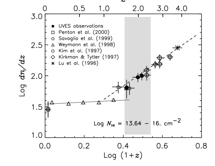
Figure 5: The number density evolution of the Ly$\alpha$ forest. The column density range $N_{H\textsc{i}}=10^{13.64-16}\ {\rm cm}^{-2}$ has been chosen to allow a comparison with the HST results from Weymann et al. (wey98 (1998)), which are shown as open triangles. Filled symbols are estimated from HE0515–4414 at $<\!z\!>\ =1.61$, from J2233–606 at $<\!z\!>\ =1.98$ and from HE2217–2818 at $<\!z\!>\ =2.13$, respectively. The star, open circles, and the diamond are taken from the HIRES data at similar resolutions by Lu et al. (lu96 (1996)), Kim et al. (kim97 (1997)), and Kirkman & Tytler (kir97 (1997)), respectively. The square and pentagons are taken from Penton et al. (pen00 (2000)) and Savaglio et al. (sav99 (1999)), respectively, over $N_{H\textsc{i}}\geq 10^{14}\ {\rm cm}^{-2}$. Horizontal solid lines represent the $z$ interval over which the number density was estimated. Vertical solid lines represent the $1\sigma$ Poisson errors. The shaded area is the $z$ range where UVES is extremely sensitive. The long-dashed line is the maximum likelihood fit to the UVES and the HIRES data at $z>1.5$. The UVES observations indicate that the number density evolution of the Ly$\alpha$ forest at $z>2.4$ continues at least down to $z\sim 1.5$ and that a slope change occurs at $z\sim 1.2$.

Fig. 6 is similar to Fig. 5, except for the $N_{H\textsc{i}}$ range: $N_{H\textsc{i}}=10^{13.1-14}\ \mathrm{cm}^{-2}$. The correction for incompleteness due to line blending is still negligible in this column density range (Fig. 4 shows that the number of lines per unit column density over $N_{H\textsc{i}}=10^{13.1-14}\ \mathrm{cm}^{-2}$ is still well represented by a single power-law). Again, the square from Penton et al. (pen00 (2000)) is estimated from the equivalent widths with the assumed $b=25$ km s^-1. The dot-dashed line is the maximum-likelihood fit to the lower column density forest of the UVES and the HIRES data: $dn/dz=(55.91\pm 2.00)\,(1+z)^{1.10\pm 0.21}$. At $2.4<z<4$ and at $2.1<z<4$, $\gamma=0.90\pm 0.29$ and $\gamma=1.00\pm 0.22$, respectively. For the column density range $N_{H\textsc{i}}=10^{13.1-14}\ \mathrm{cm}^{-2}$, the forest does not show any strong evolution.

Note that the point at $<\!z\!>\ =2.66$ (diamond) from Kirkman & Tytler (kir97 (1997)) indicates a number density twice as large as than at $<\!z\!>\ =2.87$ in the interval $N_{H\textsc{i}}=10^{13.1-14.0}\ \mathrm{cm}^{-2}$ (excluding the $<\!z\!>\ =2.66$ forest, the maximum-likelihood fit becomes $dn/dz=(47.77\pm 1.84)\,(1+z)^{1.18\pm 0.22}$). Although this discrepancy could result from a real cosmic variance of the number density from sightline to sightline, the number density in the interval $N_{H\textsc{i}}=10^{13.64-16.0}\ \mathrm{cm}^{-2}$ from the same line of sight is in good agreement with other HIRES data. The differential density distribution function (Fig. 4) and the mean H i opacity (Fig. 15) towards this line of sight suggest that the discrepancy at $N_{H\textsc{i}}=10^{13.1-14.0}\ \mathrm{cm}^{-2}$ is due to overfitting, which, as discussed in Sect. 3, may occur especially in high S/N data.

As previously noticed (Kim et al. kim97 (1997)), the lower column density forest evolves at a slower rate than the higher column density forest. The evolutionary rate $\propto(1+z)^{1.10\pm 0.21}$ would be consistent with no evolution for $q_{\mathrm{o}}=1$ or mild evolution for $q_{\mathrm{o}}=0.5$. For $\Omega_{\Lambda}=0.7$, $\Omega_{\mathrm{m}}=0.3$ and $\Omega=1$, the Ly$\alpha$ forest with $N_{H\textsc{i}}=10^{13.1-14}\ \mathrm{cm}^{-2}$ is mildly evolving at $z>1.5$. The Ly$\alpha$ forest with $N_{H\textsc{i}}=10^{13.1-14}\ \mathrm{cm}^{-2}$ appears more numerous at $z\sim 0$ than expected when extrapolating from the $z>1.5$ range.

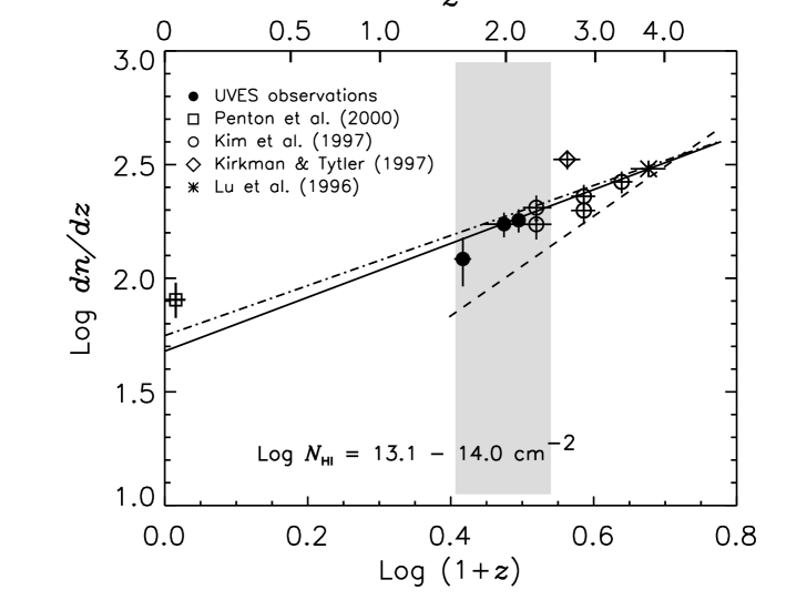
Figure 6: The number density evolution of the Ly$\alpha$ forest at the $N_{H\textsc{i}}$ range $N_{H\textsc{i}}=10^{13.1-14.0}\ \mathrm{cm}^{-2}$. Symbols are the same as in Fig. 5. The dot-dashed line (solid line) is the maximum likelihood fit to the lower column density forest including the $<\!z\!>\,=2.66$ forest (excluding the $<\!z\!>\,=2.66$ forest), while the dashed line represents the maximum likelihood fit to the forest at $N_{H\textsc{i}}=10^{13.64-16}\ \mathrm{cm}^{-2}$ from Fig. 5.

4.3 The lower cutoff $b$ in the $N_{H\textsc{i}}$–$b$ distribution

4.3.1 The lower cutoff $b$ parameter

For a photoionized gas, a temperature-density relation exists, i.e. the equation of state: $T=T_{\mathrm{0}}\,(1+\delta)^{\gamma_{T}-1}$, where $T$ is the gas temperature, $T_{0}$ is the gas temperature at the mean gas density, $\delta$ is the baryon overdensity, $(\rho_{b}-\overline{\rho}_{b})/\overline{\rho}_{b}$ ($\overline{\rho}_{b}$ is the mean baryon density), and $\gamma_{T}$ is a constant which depends on the reionization history (Hui & Gnedin hui97a (1997)). For an abrupt reionization at $z\gg 5$, the temperature of the mean gas density decreases as $z$ decreases after the reionization, eventually approaching an asymptotic $T_{\mathrm{0}}$. For a generally assumed QSO-dominated UV background with a sudden turn-on of QSOs at $5<z<10$, $T_{0}$ decreases as $z$ decreases at $2<z<4$ (Hui & Gnedin hui97a (1997)).

Under the assumption that there are some lines which are broadened primarily by the thermal motion at any given column density, this equation of state translates into a lower cutoff $b(N_{H\textsc{i}})$ envelope in the $N_{H\textsc{i}}$–$b$ distribution: $T$ and $\delta$ can be derived from $b$ and $N_{H\textsc{i}}$. For the equation of state $T=T_{0}\,(1+\delta)^{\gamma_{T}-1}$, $b_{c}(N_{H\textsc{i}})$ becomes

$$\log(b_{c})=\log(b_{0})+(\Gamma_{T}-1)\,\log(N_{H\textsc{i}}),$$ (1)

where $\log(b_{0})$ is the intercept of the cutoff in the $\log(N_{H\textsc{i}})$-$\log b$ diagram and $(\Gamma_{T}-1)$ is the slope of the cutoff (Schaye et al. sch99 (1999)). The cutoff slope $(\Gamma_{T}-1)$ is proportional to $(\gamma_{T}-1)$. This cutoff envelope provides a probe of the gas temperature of the IGM at a given $z$, thus giving a powerful constraint on the thermal history of the IGM (Hu et al. hu95 (1995); Lu et al. lu96 (1996); Kim et al. kim97 (1997); Kirkman & Tytler kir97 (1997); Zhang et al. zha97 (1997); Schaye et al. sch99 (1999); Bryan & Machacek bry00 (2000); McDonald et al. mc00 (2000); Ricotti et al. ric00 (2000); Schaye et al. sch00 (2000)).

In practice, defining $b_{c}(N_{H\textsc{i}})$ in an objective manner is not trivial due to the finite number of available absorption lines, sightline-to-sightline cosmic variances, limited S/N, and unidentified metal lines. Among several methods proposed to derive $b_{c}(N_{H\textsc{i}})$, we have adopted the following three: the iterative power-law fit, the power-law fit to the smoothed $b$ distribution, and the $b$ distribution. We refer the reader to other papers for more methods to derive $b_{c}(N_{H\textsc{i}})$ (Hu et al. hu95 (1995); McDonald et al. mc00 (2000); Theuns & Zaroubi the00 (2000)).

In our analysis, we divide the data points into 2 groups: Sample A and Sample B. Sample A consists of the lines in the range $N_{H\textsc{i}}=10^{12.5-14.5}\ \mathrm{cm}^{-2}$ with errors less than 25% in both $N_{H\textsc{i}}$ and $b$ in order to avoid ill-fitted values from VPFIT. Sample B consists of all the lines with $N_{H\textsc{i}}=10^{12.5-14.5}\ \mathrm{cm}^{-2}$ regardless of errors. The criteria for Sample A and Sample B are chosen to compare our results with the previous results by Schaye et al. (sch00 (2000)) and to investigate whether it is reasonable to include the Q0302–003 line list for which error estimates are not given. As no errors are available for Q0302–003, no Sample A can be defined at $<\!z\!>\ =2.87$. Note that including the relatively few lines with $N_{H\textsc{i}}=10^{14.5-16}\ \mathrm{cm}^{-2}$ does not change the results significantly. There is hardly any overlap in $z$, except for J2233-606 and HE2217-2818. Since one of our aims is to probe the $z$-evolution of $b_{c}(N_{H\textsc{i}})$, we analyze the $b$ distribution of each line of sight individually to derive $b_{c}(N_{H\textsc{i}})$.

Figure 7: The $\log N_{H\textsc{i}}$–$b$ diagrams with the power law fits over $N_{H\textsc{i}}=10^{12.5-14.5}\ \mathrm{cm}^{-2}$. Errors are not displayed. Crosses indicate the data points with errors less than 25% both in $N_{H\textsc{i}}$ and $b$ (Sample A), while open circles indicate the lines with errors greater than 25 % (Sample B consists of crosses and open circles together). At $<\!z\!>\ =2.87$, no Sample A can be defined due to the lack of errors in the line list. Thus, Sample B was used as a substitute for Sample A when compared to Sample A from QSOs at other $z$. The solid line, the dot-dashed line and the dashed line at each panel indicate the power law fit to Sample A, to Sample B and to the $<\!z\!>\ =3.75$ forest for comparisons, respectively. At $<\!z\!>\ =2.87$ the solid line is not present since no Sample A can be defined.

4.3.2 The iterative power law fit

Since the equation of state is a power law, it is reasonable to fit $N_{H\textsc{i}}$–$b_{c}$ with one. We did so, using the bootstrap method described by Schaye et al. (sch99 (1999)), iterating until convergence was reached. After each iteration, those points were excluded that lay more than one mean absolute deviation above the fit. Finally, the lines more than one mean absolute deviation below the fit were also taken out and the final power law fit, $b_{c}=c_{0,p}\,N_{H\textsc{i}}^{\Gamma_{T}-1}$, was carried out. The procedure was repeated over 200 bootstrap realizations in order to determine the full probability distribution of the parameters of the cutoff. As noted by Schaye et al. (sch00 (2000)), the power law fit requires over 200 available lines to reach stable fit parameters.

Fig. 7 shows the iterative power law fit in the $\log N_{H\textsc{i}}$–$b$ distributions. The noticeable difference between Sample A (cross symbols) and Sample B (cross symbols and open circles) occurs at $N_{H\textsc{i}}\leq 10^{13}\ \mathrm{cm}^{-2}$. These lines usually come from blends or from weak, asymmetric absorption lines. Table 4 lists the fitted parameters, such as $c_{0,p}$ and $(\Gamma_{T}-1)$, including $b_{c}$ values at the fixed column density $N_{H\textsc{i}}=10^{13.5}\ \mathrm{cm}^{-2}$, $b_{c,13.5}$, for Sample A and Sample B.

The power law fit between Sample A and Sample B does not give a significant difference except at $<\!z\!>\ =2.13$ and at $<\!z\!>\ =3.75$, for which several lines with $b\leq 20$ km s^-1 and $N_{H\textsc{i}}\leq 10^{13}\ \mathrm{cm}^{-2}$ contribute to a different power law fit for Sample B. This suggests that using the Q0302–003 line list at $<\!z\!>\ =2.87$ without error bars does not severely distort our conclusions. Note that the power law fit at $<\!z\!>\ =2.87$ might be less steep with a higher intercept, if the same general behavior of errors also occurs for the Q0302–003 forest (larger errors at $b\leq 20$ km s^-1 or $b\geq 40$ km s^-1). Due to the small number of lines (47 lines for Sample A and 56 lines for Sample B) at $<\!z\!>\ =1.61$, the power law fit should be taken as an upper limit on $b_{c}(N_{H\textsc{i}})$ and indeed it provides the highest $b_{c,13.5}$ among all the $z$ bins. For both Sample A and Sample B, there is a weak trend of increasing $b_{c,13.5}$ as $z$ decreases, except at $<\!z\!>\ =2.87$ which shows a higher $b_{c,13.5}$ value than at the adjacent $z$ ranges (see Sect. 6.2 for further discussion). On the other hand, the power law slope $(\Gamma_{T}-1)$ is rather ill-defined with $z$ with a possible flatter slope at $<\!z\!>\ =3.75$ than at $z<3.1$.

Fig. 8 shows the power law fit to Sample A at $z\sim 2.1$ (small filled circles; 242 lines from J2233–606 and HE2217–28118) and at $<\!z\!>\ =3.75$ (open squares; 209 lines) over $N_{H\textsc{i}}=10^{12.5-14.5}\ \mathrm{cm}^{-2}$ (upper panel) and over $N_{H\textsc{i}}=10^{13-14.5}\ \mathrm{cm}^{-2}$ (lower panel). The fitted parameters are given in Table 4. For both $N_{H\textsc{i}}$ ranges, the slopes of $b_{c}(N_{H\textsc{i}})$ are steeper at $z\sim 2.1$ than at $<\!z\!>\ =3.75$. This result, however, is certainly biased by the lack of lines with $b\leq 15$ km s^-1 and $N_{H\textsc{i}}\leq 10^{13.4}\mathrm{cm}^{-2}$ at higher $z$, due to the severe line blending.

Table 4: The power law fit to the $N_{H\textsc{i}}$–$b$ distributions

	Sample A					Sample B
$<\!z\!>$	#a	$\log(c_{0,p})$	$(\Gamma_{T}-1)$	$b_{c,13.5}$ (km s-1)b		#a	$\log(c_{0,p})$	$(\Gamma_{T}-1)$	$b_{c,13.5}$ (km s-1)b
1.61	47	$-0.92\pm 0.09$	$0.17\pm 0.01$	$24.5\pm 2.4$		56	$-0.87\pm 0.10$	$0.17\pm 0.01$	$24.9\pm 1.1$
1.98	103	$-0.49\pm 0.11$	$0.14\pm 0.01$	$21.4\pm 0.5$		146	$-0.43\pm 0.12$	$0.13\pm 0.01$	$21.4\pm 0.6$
2.13	139	$0.11\pm 0.08$	$0.09\pm 0.01$	$20.1\pm 0.6$		181	$-0.70\pm 0.11$	$0.15\pm 0.01$	$20.6\pm 0.5$
2.66	140	$-0.55\pm 0.10$	$0.14\pm 0.01$	$19.6\pm 1.1$		204	$-0.13\pm 0.10$	$0.10\pm 0.01$	$18.7\pm 0.5$
2.87	-	-	-	-		223	$-0.89\pm 0.08$	$0.16\pm 0.01$	$20.4\pm 0.8$
3.75	209	$0.51\pm 0.06$	$0.06\pm 0.01$	$18.7\pm 1.2$		271	$0.71\pm 0.10$	$0.04\pm 0.01$	$17.1\pm 0.9$
2.1c	242	$-0.22\pm 0.08$	$0.11\pm 0.01$	$19.6\pm 0.6$		327	$-0.73\pm 0.08$	$0.15\pm 0.01$	$20.4\pm 0.5$
2.1d	156	$-0.64\pm 0.13$	$0.15\pm 0.01$	$21.2\pm 0.7$		187	$-0.78\pm 0.12$	$0.16\pm 0.01$	$20.9\pm 0.6$
3.75e	188	$0.09\pm 0.10$	$0.09\pm 0.01$	$18.9\pm 1.0$		233	$-0.06\pm 0.09$	$0.10\pm 0.01$	$18.1\pm 0.9$

• The number of absorption lines used for the fit.

• The errors were estimated from the difference between the mean $b_{c,13.5}$ and the minimum/maximum $b_{c,13.5}$ from the 200 bootstrap realizations for the given $N_{H\textsc{i}}$–$b$ pairs. The typical $1\sigma$ of the $b_{c,13.5}$ distribution from the 200 bootstrap realizations is $\sim 0.3$ km sec^-1, which is underestimated (cf. Schaye et al. sch00 (2000)).

• Combined line lists from J2233–606 and HE2218-2817. The power law fit was carried out for $N_{H\textsc{i}}=10^{12.5-14.5}\ \mathrm{cm}^{-2}$.

• Combined line lists from J2233–606 and HE2218-2817. The power law fit was carried out for $N_{H\textsc{i}}=10^{13-14.5}\ \mathrm{cm}^{-2}$.

• For $N_{H\textsc{i}}=10^{13-14.5}\ \mathrm{cm}^{-2}$.

Figure 8: The $\log N_{H\textsc{i}}$–$b$ diagrams with the power law fits at $z\sim 2.1$ (only for J2233–606 and HE2217–2818; small filled circles) and at $<\!z\!>\ =3.75$ (open squares). At both redshifts, the data points with errors less than 25% in both $N_{H\textsc{i}}$ and $b$ are displayed. The upper panel shows the fit to the column density range $N_{H\textsc{i}}=10^{12.5-14.5}\ \mathrm{rm}^{-2}$, while the lower panel is to the range $N_{H\textsc{i}}=10^{13-14.5}\ \mathrm{rm}^{-2}$. The vertical dotted lines in each panel represent the column density range over which the power law fit was carried out. The solid line shows the power law fit at $z\sim 2.1$, and the dashed line at $z=3.75$. A deficit of lines with $N_{H\textsc{i}}\leq 10^{13}\ \mathrm{cm}^{-2}$ and $b\leq 20$ km s^-1 observed at $<\!z\!>\ =3.75$ is due in part to the fact that all the fitted lines with $N_{H\textsc{i}}\leq 10^{13}\ \mathrm{cm}^{-2}$ and $b\leq 20$ km s^-1 have errors larger than 25 % and in part to the severe line blending which limits the detection of weak lines.

4.3.3 The power law fit to the smoothed $b$ distribution

Bryan & Machacek (bry00 (2000)) presented a method to measure $b_{c}(N_{H\textsc{i}})$ from a power law fit to a smoothed $b$ distribution, sorting absorption lines by $N_{H\textsc{i}}$ and then dividing them into groups containing similar numbers of lines. The $b$ distribution in each group was then smoothed with a Gaussian filter with a smoothing constant $\sigma_{b}$:

$$S_{b,j}(b)=\sum_{i}\exp(-(b_{i}-b)^{2}/2\sigma_{b}^{2}),$$ (2)

where $S_{b,j}(b)$ is the smoothed density of lines in each group $j$ and $i$ indicates the lines in the group. Then, the location of the first peak in the derivative of $S_{b,j}(b)$ defines the lower cutoff at the average column density, $N_{{H\textsc{i}},j}$, for the $j$-th group.

Fig. 9 shows the $\log N_{H\textsc{i}}$–$b$ diagram at each $z$ with the $b_{c}(N_{H\textsc{i}})$ points for each group (filled circles) measured from the smoothed $b$ distributions. We use the smoothing constant $\sigma_{b}=3$ km s^-1. However, $S_{b,j}(b)$ is largely insensitive to the smoothing constant. In general, 30 lines were included in each group except for the last group at higher $N_{H\textsc{i}}$ for which typically smaller numbers of lines were available. For this same reason, at $<\!z\!>\ =1.61$ groups of $\sim 16$ lines were used. The solid line represents the robust least-squares power law fit to filled circles: $b_{c}(N_{H\textsc{i}})=c_{0,s}N_{H\textsc{i}}^{\ \Gamma_{T}-1}$. Table 5 lists the parameters of the power law fit to the smoothed $b$ distributions.

We find that the power law fit to the smoothed $b$ distribution produces in general a lower intercept and a steeper slope than the iterative power law fit. It also produces smaller $b_{c,\mathrm{13.5}}$ values. Direct comparison of Fig. 9 with Fig. 7 indicates that $b_{c}(N_{H\textsc{i}})$ measured from the smoothed $b$ distribution can be considered as a lower limit on the real $b_{c}(N_{H\textsc{i}})$, while $b_{c}(N_{H\textsc{i}})$ from the iterative power law fit can be considered as an upper limit on the real $b_{c}(N_{H\textsc{i}})$.

As with the iterative power law fit, $b_{c,\mathrm{13.5}}$ measured from the smoothed $b$ distribution increases continuously as $z$ decreases, except at $<\!z\!>\ =2.87$, where $b_{c,\mathrm{13.5}}$ is higher than at the adjacent redshifts (see Sect. 6.2 for further discussion). The slope $(\Gamma_{T}-1)$ measured from the smoothed $b$ distribution also does not show any well-defined trend with $z$.

Table 5: The power law fit to the smoothed $b$ distributions

$<\!z\!>$	$\log(c_{0,s})$	$(\Gamma_{T}-1)$	$b_{c,13.5}$
			(km s-1)
1.61	$-0.92\pm 0.13$	$0.16\pm 0.04$	$20.3\pm 1.1$
1.98	$-1.42\pm 0.02$	$0.20\pm 0.01$	$19.1\pm 1.0$
2.13	$-0.93\pm 0.11$	$0.16\pm 0.03$	$18.8\pm 1.1$
2.66	$-0.73\pm 0.22$	$0.14\pm 0.06$	$16.6\pm 1.2$
2.87a	$-1.42\pm 0.08$	$0.20\pm 0.02$	$19.0\pm 1.1$
3.75	$0.16\pm 0.07$	$0.08\pm 0.02$	$16.4\pm 1.1$
2.1b	$-0.71\pm 0.14$	$0.15\pm 0.04$	$19.2\pm 1.0$
2.1c	$-0.50\pm 0.34$	$0.13\pm 0.09$	$19.7\pm 1.1$
3.75d	$-0.30\pm 0.13$	$0.11\pm 0.03$	$15.8\pm 1.0$

• For Sample B since Sample A cannot be defined.

• At $N_{H\textsc{i}}=10^{12.5-14.5}\ \mathrm{cm}^{-2}$ for J2233–606 and HE2218-2817.

• At $N_{H\textsc{i}}=10^{13-14.5}\ \mathrm{cm}^{-2}$ for J2233–606 and HE2218-2817.

• At $N_{H\textsc{i}}=10^{13-14.5}\ \mathrm{cm}^{-2}$.

Figure 9: The $\log N_{H\textsc{i}}$–$b$ diagrams for Sample A at each $z$ (Sample B at $<\!z\!>\ =2.87$) with the robust least-squares power law fit to the smoothed $b$ distribution with the Gaussian smoothing constant 3 km s^-1. Small open squares represent the data points for Sample A (Sample B at $<\!z\!>\ =2.87$), while filled circles represent the cutoff $b$ values estimated from the smoothed $b$ distributions with $\sim 30$ lines in each group (see the text for the details). The solid line represents the robust least-squares power law fit to filled circles.

4.3.4 The $b$ distributions

Assuming that absorption lines arise from local optical depth ($\tau$) peaks and that $\ln\tau$ is a Gaussian random variable, Hui & Rutledge (hui99 (1999)) derived a single-parameter $b$ distribution:

$$dn/db=B_{\mathrm{HR}}\,\frac{{b_{\sigma}}^{4}}{b^{5}}\,\exp(-\frac{{b_{\sigma}}^{4}}{b^{4}}),$$ (3)

where $n$ is the number of absorption lines, $B_{\mathrm{HR}}$ is a constant and $b_{\mathrm{\sigma}}$ is a parameter determined by the average amplitude of the fluctuations and the effective smoothing scale.

Fig. 10 shows the observed $b$ distributions at each $z$. The noticeable difference between Sample A (solid lines) and Sample B (dot-dashed lines) occurs at $b\leq 20$ km s^-1 or $b\geq 40$ km s^-1. These unphysical lines are usually introduced by VPFIT to fit noises so that the overall profile of H i forest complexes could be improved. The dashed line represents the best-fitting Hui–Rutledge $b$ distribution, while the dotted line represents the $b$ parameter for which the Hui-Rutledge $b$ distribution function vanishes to $10^{-4}$, $b_{\mathrm{HR}}$, i.e. the truncated $b$ value for the Hui-Rutledge $b$ distribution function. The parameter $b_{\mathrm{HR}}$ cannot be considered equivalent to the cutoff $b_{c}$ since it is derived from the $b$ distribution without assuming the $b_{c}$ dependence on $N_{H\textsc{i}}$. It is more sensitive to smaller $b$ values in the $b$ distribution, which are in general coupled with lower $N_{H\textsc{i}}$. Table 6 lists the relevant parameters describing the Hui-Rutledge $b$ distribution for Sample A, such as the constant $B_{\mathrm{HR}}$, $b_{\sigma}$, $b_{\mathrm{HR}}$ and the median $b$ values at different column density ranges.

It is hard to specify subtle differences among the $b$ distributions: while the modal $b$ value and the $b_{\mathrm{HR}}$ value have a minimum at $<\!z\!>\ =3.75$, they have a maximum at $<\!z\!>\ =2.87$. The $<\!z\!>\ =2.87$ forest also has the broadest $b$ distribution. However, this large $\sigma(b)$ could be in part due to a different fitting program and in part due to a lack of information on the errors. Other parameters, such as $b_{\sigma}$, $b_{\mathrm{HR}}$, and $\sigma(b)$, appear to be fairly constant with $z$.

Figure 10: The $b$ distribution of the Ly$\alpha$ forest at each $z$. While solid lines are for Sample A, dot-dashed lines are for Sample B (no Sample A at $<\!z\!>\ =3.75$). The dashed line and the dotted line represent the best-fitting Hui-Rutledge function and $b_{\mathrm{HR}}$, respectively. The $b_{\mathrm{med}}$ value in the panels indicates the median $b$ value at the corresponding $z$ for Sample A. The number in parentheses indicates the $1\sigma(b)$ value from the Gaussian distribution.

Figure 11: The $b$ distribution as a function of $z$ for Sample A (Sample B at $<\!z\!>\ =3.75$). The horizontal dashed line indicates $b=20$ km s^-1 which is a $N_{H\textsc{i}}$-independent $b_{c}$ at $z\sim 2.8$ (Hu et al. hu95 (1995)). Circles, crosses, diamonds, stars, triangles and squares are from HE0515–4414, J2233–606, HE2217–2818, HS1946+7658, Q0302–003 and Q0000–263, respectively. There is an indication of increasing $b_{c}$ with decreasing $z$ at $z\sim 3.7$. At $z<3.1$, $b_{c}$ is not clearly defined.

Fig. 11 shows the $b$ distribution with $z$. This diagram does not assume a $b_{c}$ dependence on $N_{H\textsc{i}}$, but is sensitive to a local $b_{c}(N_{H\textsc{i}})$ variance. At $z<3.1$, there is no clear indication of the behavior of the lower cutoff $b$ values as a function of $z$. However, there is a clear indication of a trend with $z$ of the lower cutoff $b$ values over $3.5<z<3.9$. In Fig. 11, there are distinct regions at $1.8<z<2.4$. The apparent cutoff values in $b$ at $2.2<z<2.4$ and at $1.8<z<1.9$ are clearly higher than at $1.9<z<2.2$. The $2.2<z<2.4$ region towards HE2217–2818 corresponds to a $\sim 44\,h^{-1}$ Mpc void (the region B in Fig. 14), which might suggest enhanced ionization due to a nearby QSO or processes of galaxy formation (Theuns et al. 2000a ).

Table 6: The parameters of the $b$ distributions

$<\!z\!>$	$B_{\mathrm{HR}}$	$b_{\sigma}$	$b_{\mathrm{HR}}$	$b_{\mathrm{med}}^{\mathrm{a}}$	$b_{\mathrm{med}}^{\mathrm{b}}$
		(km s-1)	(km s-1)	(km s-1)	(km s-1)
1.61	7.37	23.01	12.61	28.14	34.56
1.98	7.98	23.83	13.04	26.04	29.10
2.13	7.46	23.61	12.95	25.34	29.57
2.66	6.82	24.09	13.25	28.30	30.10
2.87	7.09	27.75	15.30	28.74	34.05
3.75	6.72	22.41	12.31	28.90	30.70

• For lines with $N_{H\textsc{i}}=10^{13.1-14}\ \mathrm{cm}^{-2}$ from Sample A (Sample B at $<\!z\!>\ =2.87$).

• For lines with $N_{H\textsc{i}}=10^{13.8-16}\ \mathrm{cm}^{-2}$ from Sample A (Sample B at $<\!z\!>\ =2.87$).

4.4 The two-point velocity correlation function

The Ly$\alpha$ forest contains information on the large-scale matter distribution and the simplest way to study it is to compute the two-point velocity correlation function, $\xi(\Delta v)$. The correlation function compares the observed number of pairs ($N_{\mathrm{obs}}$) with the expected number of pairs ($N_{\mathrm{exp}}$) from a random distribution in a given velocity bin ($\Delta v$): $\xi(\Delta v)=N_{\mathrm{obs}}(\Delta v)/N_{\mathrm{exp}}(\Delta v)-1$, where $\Delta v=c\,(z_{2}-z_{1})/[1+(z_{2}+z_{1})/2]$, $z_{1}$ and $z_{2}$ are redshifts of two lines and $c$ is the speed of light (Cristiani et al. cri95 (1995); Cristiani et al. cri97 (1997); Kim et al. kim97 (1997)).

Studies of the correlation function of the Ly$\alpha$ forest have generally led to conflicting results even at similar $z$. Some studies find a lack of clustering (Sargent et al. sar80 (1980) at $1.7<z<3.3$; Rauch et al. rau92 (1992) at $z\sim 3$; Williger et al. wil94 (1994) at $z\sim 4$), while others find clustering at scales $\Delta v\leq 350$ km s^-1 (Webb web87 (1987) at $1.9<z<2.8$; Hu et al. hu95 (1995) at $z\sim 2.8$; Kulkarni et al. kul96 (1996) at $z\sim 1.9$; Lu et al. lu96 (1996) at $z\sim 3.7$; Cristiani et al. cri97 (1997) at $z\sim 3.3$).

Figure 12: Evolution of the two-point correlation function with redshift for Ly$\alpha$ lines with column densities above $N_{H\textsc{i}}=10^{12.7}\ \mathrm{cm}^{-2}$. Short-dashed and long-dashed lines represent the $1\sigma$ and $2\sigma$ Poisson errors.

Fig. 12 shows the velocity correlation strength at $\Delta v<4\,000$ km s^-1. To obtain sufficient statistics, the analysis was carried out in three redshift bins: $1.5<z<2.4$ (HE0515–4414, J2233–606, and HE2217–2818), $2.5<z<3.1$ (HS1946+7658 and Q0302–003) and $3.5<z<4.0$ (Q0000–263).

In our approach $N_{\mathrm{exp}}$ was estimated averaging $1\,000$ numerical simulations of the observed number of lines, trying to account for relevant cosmological and observational effects. In particular a set of lines was randomly generated in the same redshift interval as the data according to the cosmological distribution $\propto(1+z)^{\gamma}$, with $\gamma=2.4$ (see Sect. 4.2). The results are not sensitive to the value of $\gamma$ adopted and even a flat distribution (i.e. $\gamma=0$) gives values of $\xi$ that differ typically by less than 0.02. Line blanketing of weak lines due to strong complexes was also accounted for. Lines with too small velocity splittings, compared with the finite resolution or the intrinsic blending due to the typical line widths–the so-called “line-blanketing” effect (Giallongo et al. gia96 (1996)), were excluded in the estimates of $N_{\mathrm{exp}}$.

Clustering is clearly detected at low redshift: at $1.5<z<2.4$ in the 100 km s^-1 bin, we measure $\xi=0.4\pm 0.1$ for lines with $N_{H\textsc{i}}\ga 10^{12.7}\ \mathrm{cm}^{-2}$. There is a hint of increasing amplitude with increasing column density: in the same redshift range $\xi=0.35\pm 0.08$ for lines with $N_{H\textsc{i}}\ga 10^{12.5}\ \mathrm{cm}^{-2}$. The trend is not significant but agrees with the behavior observed at higher redshifts (Cristiani et al. cri97 (1997); Kim et al. kim97 (1997)). Unfortunately the number of lines observed in the interval $1.5<z<2.4$ does not allow us to extend the analysis to higher column densities, although groups of strong lines are occasionally evident (e.g. the range 3230–3270 Å in HE0515–4414).

The amplitude of the correlation at $100$ km s^-1 decreases significantly with increasing redshift from $0.4\pm 0.1$ at $1.5<z<2.4$, to $0.14\pm 0.06$ at $2.5<z<3.1$ and $0.09\pm 0.07$ at $3.5<z<4.0$.

Table 7: Voids at $z\sim 2$

QSO	Region	Wavelength	$<\!z\!>$	$\Delta z$	Comoving sizea	$x_{\mathrm{gap}}$	$P_{>}(x_{\mathrm{gap}})$
		(Å)			($h^{-1}$ Mpc)
HE0515–4414	A	3088–3161	1.570	0.060	61.1	5.7	0.045
HE2217–2818	A	3504–3579	1.913	0.062	54.3	8.4	0.012
HE2217–2818	B	3878–3946	2.218	0.056	43.5	8.0	0.018

• For $q_{\mathrm{0}}=0.1$.

4.5 Voids

Voids along the three low-redshift lines of sight were searched for. For comparison with previous results (Carswell & Rees car87 (1987); Crotts cro87 (1987); Ostriker et al. ost88 (1988)), we identify a void as a region without any absorption stronger than $N_{H\textsc{i}}\sim 10^{13.5}\ \mathrm{cm}^{-2}$ over a comoving size of at least $30\,h^{-1}$ Mpc (assuming $q_{\mathrm{0}}=0.1$).

Figs. 13–14 show the voids detected in the spectrum of HE0515–4414 and HE2217–2818, respectively. No significant void was found in the spectrum of J2233–606. The wavelength range used for searching for voids has been selected to be redward of the QSO’s Ly$\beta$ emission line and $3\,000$ km s^-1 blueward of the QSO’s Ly$\alpha$ emission to avoid the proximity effect. The wavelength range searched for voids is larger than that used to study the Ly$\alpha$ forest in other sections.

Table 7 lists the dimensions of the voids, as well as the probability of finding a void larger than their comoving size. The probability was calculated assuming a Poisson distribution of the local forest. In this case, the probability of finding a void larger than a given size $x_{\mathrm{gap}}$ is $P_{>}(x_{\mathrm{gap}})=1-(1-\exp^{-x_{\mathrm{gap}}})^{n}$, where $x_{\mathrm{gap}}$ is the line interval in the unit of the local mean line interval and $n$ is the number of lines with $N_{H\textsc{i}}\geq 10^{13.5}\ \mathrm{cm}^{-2}$ (Ostriker et al. ost88 (1988)). The joint probability of finding two voids with a size larger than $40\,h^{-1}$ Mpc at $z\sim 2$, as observed in the spectrum of HE2217–2818, is of the order of $2\times 10^{-4}$. The results correspond very well to the probability estimates derived from the simulations described above.

There are different ways to produce a void in the forest: a large fluctuation in the gas density of absorbers, enhanced UV ionizing radiation from nearby faint QSOs or star-forming galaxies, feedback processes (including shock heating) from galaxy formation (Dobrzycki & Bechtold dob91 (1991); Heap et al. hea00 (2000); Theuns et al. 2000a ). We recall here that the void B in the spectrum of HE2217–2818 corresponds to a region of above-average Doppler parameter (Sect. 4.3.3). It will be interesting to carry out deep imaging around HE2217–2818 to identify QSO candidates and investigate whether a local ionizing source is responsible for the $\sim 50\,h^{-1}$ Mpc voids.

Figure 13: The spectrum of HE0515–4414 with the void at $z=1.570$. See the text for the details.

Figure 14: The spectrum of HE2217–2818 with the void regions. The voids are indicated as A at $z=1.913$ and B at $z=2.218$. See the text for the details.

5 The flux statistics on the Ly$\alpha$ forest

The traditional Voigt profile fitting analysis is limited by two major drawbacks. First, there is no unique solution. Although the $\chi^{2}$ minimization is normally applied to the fit, different fitting programs produce slightly different results. Even using the same program, different $\chi^{2}$ thresholds lead to different numbers of lines when line blending is severe. As the resolution and S/N increase, many forest lines show various degrees of departure from the Voigt profile. This departure can be fitted by adding physically improbable narrow components in high S/N data to improve the overall fit, while the same profile can usually be fitted by one broad component in low S/N data (Schaye et al. sch99 (1999); Theuns & Zaroubi the00 (2000)). Thus, it becomes harder to compare fitted line parameters from different observations and different fitting programs, as the resolution and S/N increase.

Second, there is no guarantee that absorption lines have a Voigt profile. Although searches for characteristic non-Voigt signatures have been inconclusive (Rauch rau96 (1996); Outram et al. 1999b ), numerical simulations predict non-Voigt profiles of absorption lines (Outram et al. out00 (2000)). In numerical simulations, lines are broadened by a combination of gas temperature, peculiar velocity, Hubble expansion, and Jeans smoothing (Bryan et al. bry99 (1999); Theuns & Zaroubi the00 (2000)). In conclusion, the profile fitting method should be regarded as a powerful parameterization of the spectrum, not a representation of the physics governing forest clouds (Rauch et al. rau92 (1992); Hu et al. hu95 (1995); Kirkman & Tytler kir97 (1997); Bryan et al. bry99 (1999); Schaye et al. sch99 (1999); Theuns & Zaroubi the00 (2000)).

In order to avoid the non-uniqueness of profile fitting analyses and to allow more straightforward comparisons with theoretical predictions, a direct use of observed spectra of the Ly$\alpha$ forest has been explored. The most straightforward way to characterize the observed spectra is to use the N-point functions of the transmitted flux, $F$, or the observed optical depth, $\tau$ (Miralda-Escudé et al. mir97 (1997); Rauch et al. rau97 (1997); Zhang et al. zha98 (1998); Bryan et al. bry99 (1999); Machacek et al. mac00 (2000); Theuns et al. 2000b ). In the following, we consider the one-point function and the two-point function of the transmitted flux as well as other statistical measures such as the line count and the optical depth correlation function.

For comparison with the forest at $z>2.4$, we generated artificial spectra from the published line lists. These lists are the same as those used in the Voigt profile fitting analysis in Sect. 4 (see Table 2). We added Gaussian noise to the artificial spectra, according to the quoted S/N. However, as Theuns et al. (2000b ) stated, Gaussian noise independent of flux does not represent the real, observed S/N. The difference becomes more evident at $F\sim 0$ (saturated regions), where Gaussian noise produces larger fluctuations than what is observed. Unfortunately, without details on the number of individual spectra for a given wavelength range, data reduction and the normalization of the spectra, the noise at the bottom of saturated lines cannot be simulated correctly just from the published S/N and the given CCD readout noise.

We tested our approach with two extreme cases: artificial spectra without noise and artificial spectra with Gaussian noise. Except for $F\sim 0$ at $<\!z\!>\ =3.75$, the results from these two cases do not differ significantly, in particular, at $0.1<F<0.8$ where most results are considered. We use the results from the spectra generated with Gaussian noise in this study. However, we mention any difference between these two extreme cases when it becomes noticeable. Also note that most simulations do not include noise in their analysis and, in a sense noise-free spectra would be more appropriate to be compared with the results from simulations. Due to the imperfect simulation of the noise in the artificially generated spectra, the results drawn from the flux statistics should be taken qualitatively at $F\sim 0$ and $F\sim 1$.

In order to be consistent with our profile fitting analysis, we excluded high-column-density systems with $N_{H\textsc{i}}>10^{16}\ \mathrm{cm}^{-2}$ from the spectra. Note that including these high-column-density systems does not change the general qualitative conclusions from the flux statistics. It only changes the quantitative results considerably at $z\sim 3.7$ when $F$ becomes close to 0 due to the higher number of pixels with $F\sim 0$ at $z\sim 3.7$. However, for the estimation of the mean H i opacity, we used the whole regions including high-column-density absorption systems in order to compare with the previous results from the literature (Press et al. pre93 (1993); Rauch et al. rau97 (1997)). We also remind the reader to be particularly cautious in using the line list of Q0302–003 at $z\sim 2.9$, which is the only one not generated by VPFIT. As for the Voigt fitting analysis, a systematic difference in $N_{H\textsc{i}}$ and $b$ could change the results in this Sect. at $z\sim 2.9$.

5.1 The mean H i opacity

The H i opacity, $\tau_{H\textsc{i}}(\lambda)$, is defined as $\tau_{H\textsc{i}}(\lambda)=-\ln(F_{\lambda}/F_{\mathrm{c}})$, where $\lambda$ is the observed wavelength, $F_{\lambda}$ is the observed flux at $\lambda$, and $F_{\mathrm{c}}$ is the continuum flux at $\lambda$. Since the opacity scales logarithmically, the mean opacity cannot be measured accurately when $F_{\lambda}\approx 0$. The effective opacity, $\tau_{\mathrm{eff}}$, is typically used in place of $\overline{\tau}_{H\textsc{i}}$: $\exp^{-\tau_{\mathrm{eff}}}=\ <\!\exp^{-\tau}\!>$, where $<\,\,>$ indicates the mean value averaged over wavelength. Note that the mean H i opacity and the effective H i opacity are different quantities. However, we refer to the estimated $\tau_{\mathrm{eff}}$ values as the “mean H i opacity” in this study.

Figure 15: The H i opacity as a function of $(1+z)$. Filled circles represent the mean H i opacity from the UVES data. Small triangles and diamonds represent $\overline{\tau}_{H\textsc{i}}$ from Zuo & Lu (zuo93 (1993); adding up the equivalent widths from the published line lists) and Rauch et al. (rau97 (1997); we used their $\overline{\tau}_{H\textsc{i}}^{\mathrm{cent}}$ uncorrected for continuum fitting uncertainty since all other observations were not corrected for continuum fitting uncertainties), respectively. Open circles, the star, the large square, the small diamond and the small square are estimated from the spectra generated artificially using the line list provided by Hu et al. (hu95 (1995)), Kulkarni et al. (kul96 (1996)), Lu et al. (lu96 (1996)), Kirkman & Tytler (kir97 (1997)), and Outram et al. (1999a ), respectively. Large triangles were read from Schaye et al. (sch00 (2000)). All the x-axis error bars represent the $z$ range used for the $\overline{\tau}_{H\textsc{i}}$ estimates, while the y-axis error bars were estimated from simply changing the adopted continuum by $\pm 5$%, except for large triangles whose y-axis errors were read from Schaye et al. (sch00 (2000)). The cross at $z=4.7$ (Songaila et al. son99 (1999)) and the thick diamond at $z=5.34$ (Spinrad et al. spi98 (1998)) are from the Keck II/LRIS data. The dotted line represents the commonly used formula by Press et al. (pre93 (1993)): $\overline{\tau}_{H\textsc{i}}(z)=0.0037\,(1+z)^{3.46}$, given by the conventional power law fit. The solid line represents the power law fit to the UVES and the HIRES data.

Fig. 15 shows our $\overline{\tau}_{H\textsc{i}}$ measures (in fact, the effective optical depth $\tau_{\mathrm{eff}}$), together with other opacity measures compiled from the literature. Filled circles are the $\overline{\tau}_{H\textsc{i}}$ measures from the UVES data including high-column-density absorption systems. Note that all the other opacities from the literature (except the Press et al. (pre93 (1993)) $\overline{\tau}_{H\textsc{i}}$ measurements) were measured including high-column-density regions in the spectra except damped Ly$\alpha$ systems. The Press et al. measure (dotted line) was derived at low resolution, including damped Ly$\alpha$ systems. Our experiments with the UVES data show that there is no noticeable difference between the $\overline{\tau}_{H\textsc{i}}$ measured from the spectra generated from the line lists and the $\overline{\tau}_{H\textsc{i}}$ from the observed spectra. This indicates that very weak lines do not significantly contribute to $\overline{\tau}_{H\textsc{i}}$. Therefore, the estimated $\overline{\tau}_{H\textsc{i}}$ from the spectra generated from the published line lists using high resolution, high S/N data can be considered to be reliable. In Table 8, we list the estimated $\overline{\tau}_{H\textsc{i}}$ values when these values are not given in numeric form in the relevant references of Fig. 15.

Table 8: The mean H i opacity

QSO	$<\!z\!>$	$z_{\mathrm{Ly\alpha}}$	$\tau_{H\textsc{i}}$	Ref.
HE0515–4414	1.61	1.54–1.68	0.086${}^{0.049}_{-0.051}$	This study
Q1331+170	1.85	1.68–2.01	0.064${}^{0.049}_{-0.051}$	Kulkarni et al. (kul96 (1996))
Q1100–264	1.96	1.85–2.09	0.112${}^{0.023}_{0.017}$	Schaye et al. (sch00 (2000))
J2233–606	1.98	1.80–2.17	0.161${}^{0.049}_{-0.051}$	This study
J2233–606	2.04	1.92–2.17	0.142${}^{0.049}_{-0.051}$	Outram et al. (1999a )
HE2217–2818	2.13	1.92–2.33	0.131${}^{0.049}_{-0.051}$	This study
HS1946+7658	2.66	2.50–2.81	0.234${}^{0.049}_{-0.051}$	Kirkman & Tytler (kir97 (1997)), HIRES
Q0636+680	2.80	2.58–3.02	0.298${}^{0.049}_{-0.051}$	Hu et al. (hu95 (1995)), HIRES
Q0302–003	2.87	2.63–3.11	0.275${}^{0.049}_{-0.051}$	Hu et al. (hu95 (1995)), HIRES
Q0014+813	2.97	2.74–3.20	0.289${}^{0.049}_{-0.051}$	Hu et al. (hu95 (1995)), HIRES
Q0000–263	3.75	3.48–4.02	0.733${}^{0.049}_{-0.051}$	Lu et al. (lu96 (1996)), HIRES
Q2237–061	3.84	3.69–4.02	0.75${}^{0.04}_{-0.04}$	Schaye et al. (sch00 (2000)), HIRES
Q2237–061	4.31	4.15–4.43	0.83${}^{0.06}_{-0.08}$	Schaye et al. (sch00 (2000)), HIRES

The opacity measures are dependent on the continuum fitting. For low-resolution data, the continuum is usually extrapolated from longward of the QSO’s Ly$\alpha$ emission line, typically resulting in an overestimation of the continuum, i.e. an overestimated $\overline{\tau}_{H\textsc{i}}$. On the other hand, the local continuum fitting generally adopted for high-resolution data may result in an underestimation of the continuum, i.e. an underestimated $\overline{\tau}_{H\textsc{i}}$. Therefore, it is not surprising that the $\overline{\tau}_{H\textsc{i}}$ (dotted line) from low-resolution data by Press et al. (pre93 (1993)) is higher than any other measurements. Small triangles from Zuo & Lu (zuo93 (1993)) were estimated from the published line lists using intermediate resolution data, which usually do not include low column density lines. Thus, the Zuo & Lu estimates are about a factor of 2 lower than the PRS formula at $z\sim 3$. Other observations fall inbetween the PRS formula and the Zuo & Lu values.

There is a scatter in $\overline{\tau}_{H\textsc{i}}$ at similar $z$, even though opacities are estimated from data with the same instrument configuration and reduction, such as two filled circles at $z\sim 2.1$ from UVES and three open circles at $z\sim 2.8$ from HIRES. This scatter could result from measurement errors, such as the continuum fitting, and from a cosmic spatial variance. The continuum fitting becomes unreliable at $z>3$ due to severe line blending. On the other hand, the cosmic variance is present at all $z$. For example, the difference between two UVES measurements at $z\sim 2.1$ (filled circles) is due to the two high-column-density systems with $N_{H\textsc{i}}\geq 10^{17}\ \mathrm{cm}^{-2}$ towards J2233–606. When these high-column-density systems are excluded, the opacity at $<\!z\!>\,=1.98$ (J2233–606) becomes 0.123, which is similar to the one at $<\!z\!>\,=2.13$ (HE2217–2818). Similarly, the higher opacity at $z\sim 2.80$ towards Q0636+680 is due to several high-column-density clouds on this line of sight, while two other lines of sight at $z\sim 2.8$ are relatively devoid of high-column-density clouds. Despite the same HIRES configurations, the $\overline{\tau}_{H\textsc{i}}$ values from Hu et al. (hu95 (1995)) and from Kirkman & Tytler (kir97 (1997)) are a factor of 1.2 lower than the Rauch et al. values. Since the line lists for the Rauch et al. QSO sample are not published, we cannot test whether the presence of high-column-density systems in their sample causes the higher $\overline{\tau}_{H\textsc{i}}$.

The solid line represents the least-squares fit to the UVES and the HIRES data: $\overline{\tau}_{H\textsc{i}}(z)=0.0030\pm 0.0008\,(1+z)^{3.43\pm 0.17}$. The new UVES data at $1.5<z<2.4$ suggest that $\overline{\tau}_{H\textsc{i}}$ can be well approximated by a single power law at $1.5<z<4$. Two $\overline{\tau}_{H\textsc{i}}$ measures at $z>4.5$ (cross and thick diamond) from the Keck II/LRIS data suggest that $\overline{\tau}_{H\textsc{i}}$ might be significantly higher than extrapolated from $z<4$. However, these values were derived from low-resolution data, which usually overestimate $\overline{\tau}_{H\textsc{i}}$. In fact, they correspond better to the Press et al. formula, which was also derived from low-resolution data. Without more high-resolution data at higher $z$, it is premature to conclude that the $\overline{\tau}_{H\textsc{i}}$ evolution at $z>4$ departs significantly from a single power law (cf. Schaye et al. sch00 (2000)).

In the standard Friedmann universe with the cosmological constant $\Lambda=0$, if the baryon overdensity $\delta$ is $\delta\leq 10$, the mean H i opacity can be expressed by $\overline{\tau}_{H\textsc{i}}\propto(1+z)^{3.3}/\Gamma_{H\textsc{i}}(z)$ (Machacek et al. mac00 (2000)). Although there are a few high-column-density systems in Fig. 15, our result on $\overline{\tau}_{H\textsc{i}}$, $\overline{\tau}_{H\textsc{i}}\propto(1+z)^{3.43\pm 0.17}$ at $1.5<z<4$, is in good agreement with the predicted power law index. This suggests that $\Gamma_{H\textsc{i}}(z)$ does not strongly evolve over this $z$ range.

5.2 The one-point function of the flux

The one-point function of the flux (or the probability density distribution function of the transmitted flux), $P(F)$, is simply the number of pixels which have a flux between $F$ and $F+dF$ for a given flux $F$ over the entire number of pixels per $dF$. In other words, it is the probability density to find a pixel at a given $F$ (Miralda-Escudé et al. mir97 (1997); Rauch et al. rau97 (1997); Bryan et al. bry99 (1999); Machacek et al. mac00 (2000); Theuns et al. 2000b ).

Fig. 16 shows $P(F)$ as a function of $F$. The one-point function of the flux at $F<0$ and $F>1$ from observations is due to observational and continuum fitting uncertainties. The non-smooth $P(F)$ at $<\!z\!>\ =1.61$ is due to the small number of pixels used to calculate $P(F)$. The wider $P(F)$ profiles at $F\sim 0$ and at $z>2.4$ compared with at $z<2.4$ are due to the characteristics of Gaussian noise in the spectra generated (Theuns et al. 2000b ). For the spectra generated without noise, the $P(F)$ profiles at $z>2.4$ are narrower with higher amplitude at $F\sim 0$, but do not differ significantly from the $P(F)$ profiles in Fig. 16 at $0.2<F<0.8$.

The flattening towards $F\sim 1$ at $<\!z\!>\ =3.75$ is due to the smaller number of $F\sim 1$ pixels from the increasing forest number density at higher $z$. The one-point functions of the flux at $z\sim 2.1$ (for J2233–606 and HE2217–2818) are a factor of 1.3 higher than the sCDM model simulated by Machacek et al. (mac00 (2000)) at $0.2<F<0.6$ (this lower simulated $P(F)$ is in agreement with their lower mean H i opacity at $z\sim 2$).

After smoothing $P(F)$ at $<\!z\!>\ =1.61$ over a $dF=0.14$ bin, $P(F)$ at $F=0.2$ becomes $P(F)_{\mathrm{F=0.2}}\propto\,(1+z)^{3.86\pm 0.54}$. The flux $F=0.2$ corresponds to $N_{H\textsc{i}}\sim 3.2\times 10^{13}\ \mathrm{cm}^{-2}$ (in this study, we assume $b=30$ km s^-1). At $F=0.6$ ($N_{H\textsc{i}}=1.0\times 10^{13}\ \mathrm{cm}^{-2}$), $P(F)_{\mathrm{F=0.6}}\propto\,(1+z)^{3.26\pm 0.21}$. In short, the probability density of finding strong absorption lines (smaller $F$) shows a steeper slope than that of finding weak absorption lines (larger $F$). This is in good agreement with the result from the Voigt profile fitting analysis: the higher column density forest disappears more rapidly than the lower column density forest as $z$ decreases.

Figure 16: The one-point function of the flux, $P(F)$, as a function of $F$ at different $z$. Strong absorption lines (smaller $F$) disappear more rapidly than weak absorption lines (larger $F$) as $z$ decreases.

5.3 The two-point function of the flux

The two-point function of the flux, $P(F_{1},F_{2},\Delta v)$, is the probability of two pixels with the $\Delta v$ velocity separation having normalized fluxes $F_{1}$ and $F_{2}$. It is usually expressed as

$$\overline{\Delta F}(\Delta v,\delta F_{1})$$

$$\equiv\int_{\delta F_{1}}\,\left[\int^{\infty}_{-\infty}(F_{1}-F_{2})P(F_{1},F_{2},\Delta v)\,dF_{2}\right]\,dF_{1}/\delta F_{1},$$ (4)

where $\overline{\Delta F}(\Delta v,\delta F_{1})$ is the mean flux difference between two pixels with $F_{1}$ and $F_{2}$, which are separated by $\Delta v$. At $\Delta v>200$ km s^-1, $\overline{\Delta F}(\Delta v,\delta F_{1})$ is just the difference between the mean transmitted flux and $F_{1}$. At $30<\Delta v<100$ km s^-1, the shape of $\overline{\Delta F}(\Delta v,\delta F_{1})$ contains information on the profile shape of absorption lines. However, great care has to be exercised in the interpretation since $\overline{\Delta F}(\Delta v,\delta F_{1})$ is an average quantity (Miralda-Escudé et al. mir97 (1997); Bryan et al. bry99 (1999); Machacek et al. mac00 (2000); Theuns et al. 2000b ).

Fig. 17 shows $\overline{\Delta F}(\Delta v,\delta F_{1})$ as a function of $\Delta v$ at different $z$. The left-hand panel shows the results for the observed spectra at $z<2.4$ and the spectra generated with noise at $z>2.4$, while the right-hand panel shows the results for the spectra generated from the line lists for all $z$ without noise. There is no noticeable difference between the two panels. To be comparable with the simulations by Machacek et al. (mac00 (2000)), the flux range was chosen to be $-0.1\leq\!F\!\leq 0.1$, which corresponds to $N_{H\textsc{i}}\geq 10^{13.77}\ \mathrm{cm}^{-2}$. Over this column density range, absorption lines are in general saturated and belong to a H i complex, rather than being isolated.

The overall $z$-dependence on $\overline{\Delta F}(\Delta v,\delta F_{1})$ is not clear. At $\Delta v<30$ km s^-1, $\overline{\Delta F}(\Delta v,\delta F_{1})$ shows almost identical profiles at all $z$ except at $<\!z\!>\ =$ 1.61 and 2.87. At $<\!z\!>\ =$ 1.61 and 2.87, $\overline{\Delta F}(\Delta v,\delta F_{1})$ is wider than at any other $z$. At $\Delta v>30$ km s^-1, there is a tendency for the width of $\overline{\Delta F}(\Delta v,\delta F_{1})$ to become narrower as $z$ decreases. Following Machacek et al. (mac00 (2000)), we measured $\Delta v(0.3)$, the width of $\overline{\Delta F}(\Delta v,\delta F_{1})$ at which $\overline{\Delta F}(\Delta v,\delta F_{1})$ becomes 0.3. At $<\!z\!>\ =$ 1.61, 1.98, 2.13, 2.66, 2.87, and 3.75, $\Delta v(0.3)$ is 51.06 (51.61), 44.25 (43.15), 41.62 (44.27), 47.05 (48.54), 49.99 (50.79) and 50.95 (52.11) km s^-1 (the number in parentheses is for the spectrum generated without noise), respectively. The observed $\Delta v(0.3)$ values are larger than the predicted $\Delta v(0.3)$ values, $\sim 35$ km s^-1, from the models considered by Machacek et al. (mac00 (2000)) at $z\sim 3$.

A weak trend of decreasing $\Delta v(0.3)$ with decreasing $z$ might suggest that the gas temperature decreases as $z$ decreases. In fact, Theuns et al. (2000b ) note that at a given $z$ a simulation with a hotter gas temperature shows a wider $\overline{\Delta F}(\Delta v,\delta F_{1})$ profile than a simulation with a lower gas temperature. However, numerical simulations also show that higher $b$ values at higher $z$ may be a result of other physical processes. Variations of $\overline{\Delta F}(\Delta v,\delta F_{1})$ as a function of $z$ can be a result of increasing line blending at higher $z$ as well as a change in the gas temperature.

Figure 17: The mean flux difference, $\overline{\Delta F}(\Delta v,\delta F_{1})$, as a function of $\Delta v$ at different $z$. Since $\overline{\Delta F}(\Delta v,\delta F_{1})$ is an averaged quantity, it is not obvious to interpret $\overline{\Delta F}(\Delta v,\delta F_{1})$ to be a strong indicator of the temperature of the IGM.

5.4 Line counts of the Ly$\alpha$ forest

The line count at a given flux $F_{t}$ is defined as the number of regions below $F_{t}$ (Miralda-Escudé et al. mir96 (1996)). The number defined this way is more straightforward to determine than the conventional line counting from the profile fitting.

Figure 18: The line counts of the Ly$\alpha$ forest. The upper panel shows the normalized flux as a function of the filling factor. The lower panel represents the line counts from the observed spectra and the spectra generated with noise, which were smoothed with a 20 km s^-1 box-car function in order to decrease noise.

The upper panel of Fig. 18 shows the normalized flux of the observed spectra and the spectra generated with noise as a function of the filling factor. The filling factor is the fraction of the spectrum occupied by the pixels whose normalized flux is smaller than a given $F_{t}$. Since this method is sensitive to noise, the spectra were smoothed with a 20 km s^-1 box-car function. Except at $<\!z\!>\ =3.75$ (the broad feature at the filling factor close to 0 is due to the characteristics of Gaussian noise, i.e. larger root-mean-square fluctuations than the real, observed fluctuations at $F\sim 0$), the line counts are similar when the filling factor is 0.07–0.3. This range of the filling factor corresponds to $0.2<F<0.9$ at $z\sim 1.8$ and to $0.05<F<0.8$ at $z\sim 2.7$, i.e. pixels with a wide range of fluxes are considered. However, the same filling factor range only probes $0<F<0.3$ at $<\!z\!>\ =3.75$, where only strong lines are counted. This results in the different line count at $<\!z\!>\ =3.75$. When the filling factor is greater than 0.3, the line counts deviate from each other. This regime corresponds to $F\sim 1$, where noise distorts the true line counts.

Fig. 19 shows the line counts as a function of the filling factor again. In this diagram, the line counts were calculated using the artificial spectra generated from the fitted line lists for each QSO without adding noise, i.e. they have an infinite S/N. Note that this process does not include weak lines, usually not present in the fitted line lists. Unlike the lower panel of Fig. 18, the curves describing the line counts as a function of the filling factor show a similar progression as a function of $z$ when a filling factor is smaller than $\sim 0.3$, except for $<\!z\!>\ =2.87$. The $<\!z\!>\ =2.87$ forest also shows a slightly different behavior in the filling factor-flux diagram. The flux at a given filling factor increases continuously as $z$ decreases except that the flux corresponding to a given filling factor is larger at $<\!z\!>\ =2.87$ than at $<\!z\!>\ =2.66$ for a filling factor larger than 0.5. This might indicate the real cosmic variance in the structure of the Ly$\alpha$ forest along the line of sight towards Q0302–003 (one known void towards Q0302–003 at $z\sim 3.17$ is not included in this study. Also note that the $<\!z\!>\ =2.13$ forest includes one void region). However, a similar work done by Kim (kim99 (1999)) did not show any difference in the line counts as a function of $z$ at $2.1<z<4$ when the real observed spectra including Q0302–003 were used. It is highly unlikely that the QSO sample in Kim’s work shows the same amount of systematic differences from the QSOs used in this study for all $z$. Therefore, we cast doubts on the cosmic variance as a probable reason for the different line counts at $<\!z\!>\ =2.87$. Rather, the line parameters of Q0302–003 have not been obtained with the program VPFIT and this suggests that a different behavior of the Ly$\alpha$ forest at $z\sim 2.9$ from the rest of the forest at different $z$, such as a higher $b_{c,13.5}$ than at adjacent $z$, should be taken with caution.

Since the filling factor is determined mainly by the Hubble expansion, the negligible $z$-dependence of the line counts suggests that the evolution of the forest at $1.5<z<4$ is driven mainly by the Hubble expansion (Miralda-Escudé et al. mir96 (1996)).

Figure 19: The line counts of the Ly$\alpha$ forest. The upper panel shows the normalized flux as a function of the filling factor. The lower panel represents the line counts of the spectra generated artificially from the line lists. The abrupt drops in the line counts at the larger filling factor are due to the fact that the large number of the $F=1$ pixels do not contribute to the line counts as the filling factor approaches 1.

5.5 The step optical depth correlation function

Miralda-Escudé et al. (mir96 (1996)) first introduced a correlation function using a pixel-by-pixel transmitted flux, which is more straightforward than the two-point velocity correlation function. Cen et al. (cen98 (1998)) developed this concept further. We analyzed the clustering properties of the Ly$\alpha$ forest, following Cen et al.’s methods (cen98 (1998)). Among their newly defined correlation functions, we only consider the step optical depth correlation. In general, the trends we found from the step optical depth correlation function hold for the other correlation functions.

The step optical depth correlation function $\xi_{\tau,s}$ is defined as

$$\xi_{\tau,s}(\Delta v)\equiv\frac{<\tau_{s}(v+\Delta v)\tau_{s}(v)>}{<\tau_{s}>^{2}}-1,$$ (5)

where the step optical depth is defined as

$$\tau_{s}(\Delta v)\equiv\left\{\begin{array}[]{r@{ , \quad}l}1&\mathrm{if}\,\,\tau_{\mathrm{obs}}(v)\geq\tau_{\mathrm{min}}\,,\\ 0&\mathrm{if}\,\,\tau_{\mathrm{obs}}(v)<\tau_{\mathrm{min}}\,.\end{array}\right.$$ (6)

Fig. 20 shows the step optical depth correlation functions $\xi_{\tau,s}(\Delta v)$ with $\tau_{\mathrm{min}}=2$ as a function of $\Delta v$. The $\tau_{\mathrm{min}}=2$ corresponds to $N_{H\textsc{i}}\sim 10^{13.6}\ \mathrm{cm}^{-2}$. Although it is difficult to detect any well-defined trend of the correlation strength at $\Delta v\leq 100$ km s^-1 in the two-point correlation functions, the step optical depth correlation functions show a strong clustering at $v<100$ km s^-1. Instead of the individual pixels, the two-point correlation function uses the fitted line lists from the Voigt profile fitting. The profile fitting usually does not deblend saturated lines (higher $\tau$ and higher $N_{H\textsc{i}}$) and is less sensitive to fitting lines at small velocity separations.

The step optical depth correlation strength increases as $z$ decreases, except at $<\!z\!>\ =2.13$ at $\Delta v\leq 50$ km s^-1. The stronger correlation strength of the $<\!z\!>\ =2.13$ forest than the $<\!z\!>\ =1.98$ forest at $\Delta v\leq 30$ km s^-1 is in part caused by the 5 strong lines clustered at 3960–4005 Å. Also the $<\!z\!>\ =2.13$ forest contains a void of $44\,h^{-1}$ Mpc.

The pixel-by-pixel correlation functions are sensitive to the S/N and resolution of the data. However, the general trend of increasing correlation strength with decreasing $z$ holds at the different S/N and resolution from the experiments of degraded UVES spectra, although the degree of the correlation strengths gets weaker as the S/N and resolution decrease. With higher $\tau_{\mathrm{min}}$ values, the correlation strengths get stronger, but keep the same $z$-dependent trend. These results are in good agreement with previous findings from the two-point velocity correlation function: stronger forest lines are more strongly correlated and the correlation strengths increase with decreasing $z$ over a given column density range (Cristiani et al. cri97 (1997); Kim et al. kim97 (1997)).

Figure 20: The step optical depth correlation functions. They are sensitive to the profile shapes of the forest at the smaller velocity separations for a given $\tau_{\mathrm{min}}$.

6 Discussion

6.1 The line number density per unit redshift of the Ly$\alpha$ forest

For a given column density range, combined HST and ground-based observations have provided evidence for a change in the line number density evolution at $z\sim 1.7$: a rapid evolution at $z>1.7$ and a slow evolution at $z<1.7$ (Impey et al. imp96 (1996); Riediger et al. rie98 (1998); Weymann et al. wey98 (1998); Davé et al. dav99 (1999)). These observations have led to a speculation of two distinct populations in the Ly$\alpha$ forest: a rapidly evolving population which dominates at higher $z$ and a slowly evolving population which dominates at lower $z$.

Our results at $N_{H\textsc{i}}=10^{13.64-16}\mathrm{cm}^{-2}$ suggest that the transition from the stronger evolution to the weaker evolution in $dn/dz$ occurs at $z\sim 1.2$ (UM18 fits in the picture and is not an outlier), rather than at $z\sim 1.7$ as suggested by previous observations and numerical simulations. To be conservative, our results show that $dn/dz$ at $N_{H\textsc{i}}=10^{13.64-16}\mathrm{cm}^{-2}$ continues to decrease at a similar rate from $z=4\rightarrow 1.5$, with a suggestion of slowing down in the evolution towards lower $z$.

The physics of the Ly$\alpha$ forest at $z>2$ is determined mainly by the Hubble expansion and the ionizing background, $J_{\nu}$ (or the H i photoionization rate, $\Gamma_{H\textsc{i}}$). If the forest is “fixed” in comoving coordinates for $q_{0}=0.5$ and $\Lambda=0$, the observed number density of the Ly$\alpha$ forest is proportional to $[(1+z)^{5}\,\Gamma_{H\textsc{i}}^{-1}(z)]^{\beta-1}\,(1+z)^{-3/2}$, where $\beta$ is from $f(N_{H\textsc{i}})\propto N_{H\textsc{i}}^{-\beta}$. This implies that $dn/dz$ for a given column density threshold decreases as $z$ decreases (Miralda-Escudé et al. mir96 (1996); Davé et al. dav99 (1999)). If we assume $\beta\sim 1.5$, $dn/dz\propto(1+z)\,\Gamma_{H\textsc{i}}^{-0.5}(z)$. For a constant $\Gamma_{H\textsc{i}}$, this is much lower than the observed index of $dn/dz$, $2.19\pm 0.27$, suggesting structure evolution and/or $\Gamma_{H\textsc{i}}$ evolution in $dn/dz$.

Recent numerical simulations suggest that a decrease of $\Gamma_{H\textsc{i}}$ at $z<2$ plays a more important role to change the slope in $dn/dz$ at $z\sim 1.7$ due to the decreasing QSO luminosity function at $z<2$ (Davé et al. dav99 (1999); Riediger et al. rie98 (1998); Theuns et al. the98 (1998); Zhang et al. zha98 (1998)). The discrepancy between our observations and simulations could be due to limited box sizes at $z<2$ in most simulations (losing large-scale power), to numerical resolutions (underestimating $\tau_{H\textsc{i}}$ or the number of lines at lower $z$) or to incorrect $\Gamma_{H\textsc{i}}$. If we take the results from most simulations that $\Gamma_{H\textsc{i}}$ is the main drive of the slope change in $dn/dz$, this discrepancy could simply indicate that $\Gamma^{-1}_{H\textsc{i}}$ in most simulations, i.e. the QSO-dominated Haardt-Madau $\Gamma^{-1}_{H\textsc{i}}$ (Haardt & Madau haa96 (1996)), is underestimated at $z<2$ and that $\Gamma^{-1}_{H\textsc{i}}$ at $z<2$ changes more slowly than a QSO-dominated $\Gamma^{-1}_{H\textsc{i}}$, i.e. there is a non-negligible contribution from galaxies at $z<2$.

6.2 The $z$-evolution of $b_{c}(N_{H\textsc{i}})$

Assuming a truncated Gaussian $b$ distribution with a lower $N_{H\textsc{i}}$-independent $b_{c}$, Kim et al. (kim97 (1997)) concluded that $b_{c}$ over $N_{H\textsc{i}}=10^{12.8-16}\ \mathrm{cm}^{-2}$ increases as $z$ decreases: 15 km s^-1 at $z\sim 3.7$, 17 km s^-1 at $z\sim 3.3$, 20 km s^-1 at $z\sim 2.9$, and 22–24 km s^-1 at $z\sim 2.3$. This result has been explained by an additional heating due to the on-going He ii reionization, although the high $b_{c}$ value at $z\sim 2.3$ does not agree with any theoretical explanations (Kim et al. kim97 (1997); Haehnelt & Steinmetz hae98 (1998); Theuns et al. 2000b ; Schaye et al. sch00 (2000)).

Subsequent studies on the $z$-evolution of $b_{c}$ have led to contradictory results. While $b_{c}$ is clearly dependent on $N_{H\textsc{i}}$ (Kirkman & Tytler kir97 (1997); Zhang et al. zha97 (1997)), $b_{c}(N_{H\textsc{i}})$ and the mean $b$ value at $<\!z\!>\ =2.7$ (Kirkman & Tytler kir97 (1997)) and at $<\!z\!>\ =1.7$ (Savaglio et al. sav99 (1999)) does not show any noticeable difference compared with at $z>3$. Combining the observations with the numerical simulations, Schaye et al. (sch00 (2000)) found that $b_{c}$ at the fixed overdensity $\delta=0$, $b_{\delta=0}$, increases from $z\sim 4.5$ ($b_{\delta=0}\sim 14.5$ km s^-1) to $z\sim 3$ ($b_{\delta=0}\sim 19.5$ km s^-1) due to He ii reionization at $z\sim 3$ and then decreases from $z\sim 3$ ($b_{\delta=0}\sim 19.5$ km s^-1) to $z\sim 1.8$ ($b_{\delta=0}\sim 14$ km s^-1). Ricotti et al. (ric00 (2000)) also found a similar increase in $b_{\delta=0}$ at $z\sim 3$, although their $b_{\delta=0}$ at $z>2.8$ and at $z<2.8$ can be considered to be constant at $b_{\delta=0}\sim 14.5$ km s^-1 and at $b_{\delta=0}\sim 21$ km s^-1, respectively. On the other hand, adopting a slightly different approach for identifying absorption lines instead of the Voigt profile fitting, McDonald et al. (mc00 (2000)) found that there is no $b_{c}$ evolution over $2.1<z<4.4$ at the slightly higher overdensity $\delta=0.4$.

Fig. 21 shows the cutoff $b$ values at the fixed column density $N_{H\textsc{i}}=10^{13.5}\ \mathrm{cm}^{-2}$, $b_{c,\mathrm{13.5}}$, from the two power law fits in Sect. 4.3 as a function of $z$. Keep in mind that $b_{c}(N_{H\textsc{i}})$ from the iterative power law fit is an upper limit, while $b_{c}(N_{H\textsc{i}})$ from the smoothed $b$ distribution is a lower limit. The $b_{c,\mathrm{13.5}}$ value shows a slight increase with decreasing $z$ from both power law fits, with a possible local $b_{c,\mathrm{13.5}}$ maximum at $z\sim 2.9$ (with the caveat that the line list of Q0302–003 is generated by a different fitting program with respect to the other line lists. This could introduce an artificial result at $z\sim 2.9$ as shown in Sect. 5.4, although its redshift range suggests an influence of additional heating if He ii reionization does occur at $z\sim 3$). When all the values from both fits are averaged, $b_{c,\mathrm{13.5}}=17.6\pm 1.6$ at $z\sim 3.75$ is smaller than $b_{c,\mathrm{13.5}}=19.9\pm 1.2$ at $z\sim 2.1$, but the difference is significant only at the $1.44\sigma$ level.

In simulations, $b_{c}$ is usually measured at a fixed overdensity $\delta$ rather than at a fixed column density. Translating an overdensity into the corresponding column density is not trivial and depends on many uncertain parameters, such as the ionizing background and the reionization history. If the simple law between $\delta$ and $N_{H\textsc{i}}$ by Davé et al. (dav99 (1999)) is assumed, then $\delta$ becomes:

$$N_{H\textsc{i}}\sim\left[0.05\,(1+\delta)\,10^{0.4\,z}\right]^{1.43}\times 10^{14}\ \mathrm{cm}^{-2}.$$ (7)

For $\delta=0$, the corresponding $N_{H\textsc{i}}$ is $1.92\times 10^{14}$, $6.04\times 10^{13}$, $4.56\times 10^{13}$, $2.28\times 10^{13}$, $1.87\times 10^{13}$ and $1.15\times 10^{13}\ \mathrm{cm}^{-2}$ at $<\!z\!>\ =$ 3.75, 2.87, 2.66, 2.13, 1.98 and 1.61, respectively. Although this conversion does not include the effects of the He ii reionization, we assume that it is correct at least on a relative scale at $z\sim 3.75$ and at $z\sim 2.1$, where the He ii reionization would not affect the temperature of the IGM as strongly as at $z\sim 3$. Therefore, we only discuss the relative behavior of $b_{\delta=0}$ as a function of $z$, in particular, our $b_{\delta=0}$ at $z\sim 2.1$ with other results mentioned above.

For the iterative power law fit (the power law fit to the smoothed $b$ distribution), the $b$ value at $\delta=0$, $b_{\delta=0}$, is 20.8 (17.2), 20.1 (17.2), 19.4 (17.8), 20.5 (17.5), 22.4 (21.6) and 20.4 (18.8) km s^-1 at $<\!z\!>\ =$ 3.75, 2.87, 2.66, 2.13, 1.98 and 1.61, respectively. In the second panel of Fig. 21, $b_{\delta=0}$ is fairly constant with $z$ as $b_{\delta=0}\sim$ 17–20 km s^-1, with a possible local maximum $b_{\delta=0}\sim$ 22 km s^-1 at $z\sim 2.9$. The observed behavior of $b_{\delta=0}$ is qualitatively in agreement with the results from McDonald et al. (mc00 (2000)). While the observations agree with the fairly constant $b_{\delta=0}$ at $z<3$ derived by Ricotti et al. (ric00 (2000)), they do not show the abrupt increase of $b_{\delta=0}$ across $z\sim 3$ as large as $\sim 7$ km s^-1 found by Ricotti et al. The observations at $z\sim 3.75$ and at $z\sim 2.1$ agree with the results by Schaye et al. (sch00 (2000)) which show similar $b_{\delta=0}$ at $z\sim 3.75$ and at $z\sim 2.1$. In addition, the observations do not show a strong decrease of $b_{\delta=0}$ from $z\sim 3$ to $z\sim 2$ as large as $\sim 4$ km s^-1 as found by Schaye et al. (sch00 (2000)). However, note that, considering the large error bars of Schaye et al. (sch00 (2000)), the significance of the decrease of $b_{\delta=0}$ from $z\sim 3$ to $z\sim 2$ is not very strong and their result is not in disagreement with ours. It should also be recalled that we are using the scaling law between $\delta$ and $N_{H\textsc{i}}$ estimated from the QSO-dominated Haardt-Madau $\Gamma_{H\textsc{i}}$. If this QSO-dominated UV background is underestimated at $z<2$ as suggested by the evolution of the absorption line number density, the actual $b_{\delta=0}$ at $z<2.4$ can be higher than $b_{\delta=0}$ in Fig. 21.

The third panel of Fig. 21 shows the median $b$ values as a function of $z$ measured for two column density ranges: $N_{H\textsc{i}}=10^{13.1-14}\mathrm{cm}^{-2}$ and $N_{H\textsc{i}}=10^{13.8-16}\mathrm{cm}^{-2}$. It is rather difficult to interpret the $z$-dependence of the median $b$ values. It could be constant at $1.5<z<4$ with a small cosmic variance at $z\sim 2$. On the other hand, it could be decreasing with $z$ at $z<3.1$, if we discard the median $b$ values at $<\!z\!>\ =1.61$, based on a small number of absorption lines. Although simulations correctly predict the shape of the observed $b$ distributions, the predicted median $b$ values are typically 5–10 km s^-1 smaller than the observed ones at all $z$ (Bryan & Machacek bry00 (2000); Machacek et al. mac00 (2000); Theuns et al. 2000b ).

The bottom panel of Fig. 21 shows the power law slope of the $N_{H\textsc{i}}$–$b_{c}$ distribution, $(\Gamma_{T}-1)$, as a function of $z$ (see Eq. 1). No particular trend is apparent and $(\Gamma_{T}-1)$ shows very little evolution at $z<3.1$. Note that the lower $(\Gamma_{T}-1)$ at $<\!z\!>\ =3.75$ is in part due to the lack of lines with $b<15$ km s^-1 and $N_{H\textsc{i}}\leq 10^{13.4}\mathrm{cm}^{-2}$ (Fig. 8). When $(\Gamma_{T}-1)$ is averaged over all the measured values, $(\Gamma_{T}-1)=0.16\pm 0.03$ at $z<3.1$ is larger than $(\Gamma_{T}-1)=0.07\pm 0.02$ at $<\!z\!>\ =3.75$. Due to the lower $(\Gamma_{T}-1)$ at $<\!z\!>\ =3.75$, it also seems clear from Fig. 8 that gas at lower overdensities is cooler at $z<3.1$ than at higher $z$ (keep in mind that a fixed column density corresponds to a larger gas overdensity as $z$ decreases due to the Hubble expansion).

If we assume Eq. 7 again and $T\sim 59.2\,b^{2}$ for thermally broadened lines, $(\gamma_{T}-1)\sim 2.857\,(\Gamma_{T}-1)$. When this simple conversion law is assumed, $(\gamma_{T}-1)=0.46\pm 0.10$ at $z<3.1$ and $(\gamma_{T}-1)=0.18\pm 0.05$ at $z\sim 3.75$. These $(\gamma_{T}-1)$ could be considered to be consistent with the results by McDonald et al. (mc00 (2000)) within their error bars, although their error bars at $z=3.9$ ($(\gamma_{T}-1)=0.42\pm 0.45$) and at $z=3$ ($(\gamma_{T}-1)=0.30\pm 0.30$) are rather large. Their $(\gamma_{T}-1)=0.5\pm 0.15$ at $z\sim 2.4$ agrees with our $(\gamma_{T}-1)=0.46$. Our $(\gamma_{T}-1)$ is marginally in agreement with the results from Ricotti et al. (ric00 (2000)) and from Schaye et al. (sch00 (2000)). Their $(\gamma_{T}-1)$ values are lower at $z\sim 2$ and higher at $z\sim 3.7$, but within the error bars.

Figure 21: The $z$-evolution of $b_{c,\mathrm{13.5}}$, $b_{\delta=0}$, median $b$ and $(\Gamma_{T}-1)$ from the two power law fits in Sect. 4.3. Stars and triangles represent the parameters measured from the iterative power law fit and from the smoothed $b$ distribution, respectively. Vertical bars represent 1$\sigma$ errors. In the third panel, error bars in the x-axis represent the $z$ ranges over which the median $b$ values were estimated. Solid lines represent the median $b$ values over $N_{H\textsc{i}}=10^{13.1-14}\ \mathrm{cm}^{-2}$, while dotted lines represent the median $b$ values over $N_{H\textsc{i}}=10^{13.8-16}\ \mathrm{cm}^{-2}$.

6.3 The optical depth distribution function

While the one-point function of the flux is more closely related to observations, the one-point function of the optical depth is usually calculated in simulations (Zhang et al. zha98 (1998); Machacek et al. mac00 (2000)). In the simulation by Machacek et al. (mac00 (2000)), the H i optical depth $\tau$ at which the maximum $\tau P(\tau)$ occurs, $\tau_{\mathrm{max}}$, is $\tau\sim 0.8$ at $z=4$, $\tau\sim 0.09$ at $z=3$, and $\tau\sim 0.013$ at $z=2$. Fig. 22 shows $\tau P(\tau)$ as a function of $\tau$, which is calculated from the observed spectra at $z<2.4$ and the spectra generated with noise at $z>2.4$. The $\tau_{\mathrm{max}}$ value is $\tau\sim 0.6$ at $<\!z\!>\ =3.75$, $\tau\sim 0.13$ at $<\!z\!>\ =2.87$, and $\tau\sim 0.08$ at $<\!z\!>\ =2.66$, respectively. The observed $\tau_{\mathrm{max}}$ shows a behavior similar to the simulated results by Machacek et al. (mac00 (2000)). However, $\tau_{\mathrm{max}}$ converges to $\tau\sim 0.04$ at $z<2.4$, not showing any $z$-dependence. Also there is no $z$-dependence of $\tau P(\tau)$ at $\tau\leq 0.04$ and at $z<3.1$.

The optical depth $\tau\sim 0.04$ corresponds to $F\sim 0.96$, while $\tau\sim 0.013$ corresponds to $F\sim 0.99$, almost to the continuum level. As $z$ decreases, the number of pixels with $F=$ 0.96–0.99 increases. These pixels are noise-dominated by the limited S/N and the continuum fitting uncertainty. Therefore, instead of showing the expected $z$-dependence of $\tau_{\mathrm{max}}$ and $\tau P(\tau)$, the observed $\tau_{\mathrm{max}}$ and $\tau P(\tau)$ approach to an asymptotic $\tau_{\mathrm{max}}\sim 0.04$ value at $z<2.4$ and an asymptotic $\tau P(\tau)$ at $\tau\leq 0.04$ and at $z<3.1$, respectively.

At $0.1<\tau<3$ (or $0.05<F<0.9$), the observed $\tau P(\tau)$ is simply a different way of viewing the one-point function of the flux. As $z$ decreases, $\tau P(\tau)$ decreases due to the expansion of the universe. At $\tau>4$ (or $F<0.05$), $\tau P(\tau)$ starts to converge again since it typically samples saturated regions, again dominated by noise.

Figure 22: The $z$-evolution of $\tau P(\tau)$ as a function of $\tau$. The $\tau P(\tau)$ values are calculated from the observed spectra at $z<2.4$ and from the spectra generated with noise at $z>2.4$.

6.4 The baryon density $\Omega_{b}$

We derived the baryon density, $\Omega_{b}$, from two properties of the Ly$\alpha$ forest, $\overline{\tau}_{H\textsc{i}}$ (including all the Ly$\alpha$ forest regardless of $N_{H\textsc{i}}$) and $P(F)$ (only for the forest with $N_{H\textsc{i}}\leq 10^{16}\mathrm{cm}^{-2}$).

If $\overline{\tau}_{H\textsc{i}}\ \leq 1.24$, the lower limits on the baryon density become

$$\Omega_{b}^{\overline{\tau}_{H\textsc{i}}}\geq 5.1\times 10^{4}\,(1-\exp(-\overline{\tau}_{H\textsc{i}}))\,(1+z)^{-2.5}\,(1+\Omega_{\mathrm{0}}z)^{0.25}$$

$$\ \ \ \ \ \ \ \ \ \ \times h^{-1.75}T_{0}^{0.35}\,\Gamma_{H\textsc{i}}^{0.5},$$ (8)

where all the symbols have their usual meanings in this study (Weinberg et al. wei97 (1997)).

Table 9 lists the lower limits on $\Omega_{b}$ at different $z$, together with the parameter values used for calculating $\Omega_{b}^{\overline{\tau}_{H\textsc{i}}}$. It should be noted that the temperature used to calculate Eq. 8 is smaller than the values derived in Sect. 6.2, but in the present discussion we are only interested in the lower bounds on $\Omega_{b}$. These lower limits on $\Omega_{b}^{\overline{\tau}_{H\textsc{i}}}$ are consistent with $\Omega_{b}=0.0125\,h^{-2}$ from the Big Bang nucleosynthesis analysis (Copi et al. cop95 (1995)). These values also indicate that about 90% of all baryons reside in the Ly$\alpha$ forest at $1.5<z<4$.

The lower bounds on the density parameter from the one-point function, $\Omega_{b}^{\mathrm{P}(F)}$, are given by Weinberg et al. (wei97 (1997)) as

$$\Omega_{b}^{\mathrm{P}(F)} \geq 0.021h^{-3/2}\left(\frac{[\int^{1}_{0}(-\ln F)^{1/\beta_{\gamma}}P(F)\,dF/F]^{\beta_{\gamma}/2}}{0.70}\right)$$

$$\ \ \ \ \ \ \ \ \ \ \times\left(\frac{4}{1+z}\right)^{3}\left(\frac{H(z)/H_{\mathrm{0}}}{5.51}\right)^{1/2}\left(\frac{T_{\mathrm{0}}}{10^{4}{\mathrm{K}}}\right)^{0.35}$$

$$\ \ \ \ \ \ \ \ \ \ \times\left(\frac{\Gamma}{10^{-12}\ \mathrm{sec}^{-1}}\right)^{1/2},$$ (9)

where $\beta_{\gamma}\equiv(2-0.7\gamma_{T})^{-1}=1.6-1.8$, where $\gamma_{T}$ is the power law index of the equation of state (Weinberg et al. wei97 (1997)).

Table 9 lists the lower bounds on $\Omega_{b}^{\mathrm{P(F)}}$ along with the parameter values used to calculate $\Omega_{b}^{\mathrm{P(F)}}$. The $\Omega_{b}^{\mathrm{P(F)}}$ values are larger than $\Omega_{b}^{\overline{\tau}_{H\textsc{i}}}$ since $\overline{\tau}_{H\textsc{i}}$ is not the true mean H i opacity, but the effective opacity which underestimates the true opacity when absorption lines become saturated. The lower $\Omega_{b}$ limits from $P(F)$ are about a factor of $1.6\,h^{0.5}$ larger than the Big Bang nucleosynthesis analysis, $\Omega_{b}=0.0125\,h^{-2}$.

Our new lower bounds on $\Omega_{b}$ are a factor of 1.5 smaller than some of the previous results, $\Omega_{\mathrm{b}}=0.017$–$0.03\,h^{-2}$ (Rauch et al. rau97 (1997); Zhang et al. zha98 (1998); Burles et al. bur99 (1999); Kirkman et al. kir00 (2000); McDonald et al. mc00 (2000)), but still consistent with them within the error bars. However, our lower $\Omega_{\mathrm{b}}$ bounds are not consistent with the derived $\Omega_{b}=0.005\,h^{-2}$–$0.01\,h^{-2}$ from the high D/H measurements (Songaila et al. son94 (1994); Rugers & Hogan rug96 (1996)).

Table 9: The lower bounds on $\Omega_{b}$

$z$	$\overline{\tau}_{H\textsc{i}}$	$\Omega_{b}^{\mathrm{a}}$	$\Omega_{b}^{\mathrm{P(F),b}}$
		($\times h^{-1.75}$)	($\times h^{-1.5}$)
1.61	0.086	$\geq 0.010$	$\geq 0.020$
1.98	0.161	$\geq 0.016$	$\geq 0.021$
2.13	0.131	$\geq 0.012$	$\geq 0.021$
2.66	0.234	$\geq 0.014$	$\geq 0.020$
2.87	0.275	$\geq 0.015$	$\geq 0.020$
3.75	0.733	$\geq 0.013$	$\geq 0.013$

• For $T=6\,000$ K, $\Gamma=0.9\times 10^{-12}\ \mathrm{sec}^{-1}$ (at $z\sim 1.6$), $1.4\times 10^{-12}\ \mathrm{sec}^{-1}$ (at $z\sim$2–3), $0.64\times 10^{-12}\ \mathrm{sec}^{-1}$ (at $z\sim 3.75$), and $\Omega_{0}=1$ (Haardt & Madau haa96 (1996); Hui & Gnedin hui97a (1997); Weinberg et al. wei97 (1997)).

• For $T=6\,000$ K, $\Gamma=0.9\times 10^{-12}\ \mathrm{sec}^{-1}$ (at $z\sim 1.6$), $1.4\times 10^{-12}\ \mathrm{sec}^{-1}$ (at $z\sim$2–3), $0.64\times 10^{-12}\ \mathrm{sec}^{-1}$ (at $z\sim 3.75$), $\Omega_{0}=1$, $\beta=1.58$, and $H(z)=H_{\rm 0}\Omega_{\rm 0}^{\frac{1}{2}}(1+z)^{\frac{3}{2}}$ (Haardt & Madau haa96 (1996); Hui & Gnedin hui97a (1997); Weinberg et al. wei97 (1997)).

7 Conclusions

We have analyzed the properties of low column density Ly$\alpha$ forest clouds ($N_{H\textsc{i}}=10^{12.5-16}\mathrm{cm}^{-2}$) toward 3 QSOs at $1.5<z<2.4$, using high resolution ($R\sim 45\,000$), high S/N ($\sim$ 25–40) VLT/UVES data. Combined with other high-resolution observations from the literature at $z>2.4$, we have studied the evolution of the Ly$\alpha$ forest at $1.5<z<4$. Two parallel analyses have been applied to the datasets: the traditional Voigt profile fitting analysis and a statistical measure of the transmitted flux. We find that the general conclusions from both analyses are in good agreement. Although the results are limited by the relatively small number of lines of sight, we find the following properties and trends in the $z$-evolution of the Ly$\alpha$ forest:

1) The differential density distribution function of the lower column density forest ($N_{H\textsc{i}}=10^{12.5-14}\ \mathrm{cm}^{-2}$) does not evolve very strongly, $f(N_{H\textsc{i}})\propto N_{H\textsc{i}}^{-\beta}$, at $1.5<z<4$, with $\beta\sim 1.4$–1.5 and with an indication of an increasing $\beta$ to $\beta\sim 1.7$ at $z<1.8$. The higher column density forest ($N_{H\textsc{i}}>10^{14}\ \mathrm{cm}^{-2}$) disappears rapidly with decreasing $z$. The observed slopes of $f(N_{H\textsc{i}})$ for various column density ranges are considerably flatter than numerical predictions for the same column density thresholds. The same conclusions are drawn from the one-point function and two-point function of the flux.

2) The line number density of the Ly$\alpha$ forest with $N_{H\textsc{i}}=10^{13.64-16}\ \mathrm{cm}^{-2}$ decreases continuously from $z\sim 4$ to $z\sim 1.5$, $dn/dz\propto(1+z)^{2.19\pm 0.27}$, without showing any flattening in $dn/dz$ at $1.5<z<4$. For the lower column density range at $N_{H\textsc{i}}=10^{13.1-14}\ \mathrm{cm}^{-2}$, the number density evolution becomes weaker: $dn/dz\propto(1+z)^{1.10\pm 0.21}$. The line counts as a function of the filling factor show a negligible $z$-dependence. These results strongly suggest that the main drive in the evolution of the forest at $z>1.5$ is the Hubble expansion and that $\Gamma_{H\textsc{i}}$ changes more slowly than a QSO-dominated background at $z<2$, suggesting a contribution from galaxies to the UV background at $z<2$. When combined with the results from the HST QSO absorption line key project at $0<z<1.5$ with the same column density threshold, there is evidence for a slope change in $dN/dz$ at $z\sim 1.2$.

3) Deriving the cutoff $b_{c}(N_{H\textsc{i}})$ as a function of $z$ depends strongly on the methods used and the number of available lines. However, the cutoff $b$ parameter at the fixed column density $N_{H\textsc{i}}=10^{13.5}\ \mathrm{cm}^{-2}$, $b_{c,\mathrm{13.5}}$, shows a weak increase with decreasing $z$, with a possible local $b_{c,\mathrm{13.5}}$ maximum at $z\sim 2.9$. Despite being substantially uncertain due to the uncertain conversion from the observable parameters $b$ and $N_{H\textsc{i}}$ to the theoretical parameters $T$ and $\delta$, the cutoff $b$ value at the mean gas density, $b_{\delta=0}$, is fairly constant with $z$ as $b_{\delta=0}\sim 18$ km s^-1, with a possible local $b_{c}$ maximum at $z\sim 2.9$. The observed slopes of $b_{c}(N_{H\textsc{i}})$ do not show any well-defined $z$-dependence except for a flatter slope at $<\!z\!>\ =3.75$ than at $z<3.1$, possibly due to the severe blending of lines with low-$b$ and low-$N_{H\textsc{i}}$ at higher $z$.

4) The velocity correlation function and the step optical-depth correlation function confirm that stronger lines are more clustered than weaker lines and that the correlation strength increases as $z$ decreases.

5) The mean H i opacity is well approximated by a single power law at $1.5<z<4$, $\overline{\tau}_{H\textsc{i}}\propto(1+z)^{3.43\pm 0.17}$, without showing any flattening towards higher $z$. The significant scatter in the mean H i opacity is likely to be caused by continuum fitting uncertainty and by an inclusion/exclusion of high-column-density H i systems ($N_{H\textsc{i}}\geq 10^{17}\ \mathrm{cm}^{-2}$) towards different lines of sight.

6) The lower limit on the baryon density derived both from the H i opacity and the one-point function of the flux, $\Omega_{\mathrm{b}}^{\mathrm{Ly\alpha}}\,\sim 0.013\,h^{-1.75}$, suggests that most baryons (over 90%) reside in the forest at $1.5<z<4$. The contribution to $\Omega_{\mathrm{b}}$ from the Ly$\alpha$ forest does not change much with $z$ at $1.5<z<4$.

- (1) Bahcall, J. N., Bergeron, J., Boksenberg, A. et al., 1993, ApJS, 87, 1
- (2) Bowen, D. V., Pettini, M., Boyle, B. J., 1998, MNRAS, 297, 239
- (3) Bryan, G. L., Machacek, M. E., Anninos, P., Norman, M. L., 1999, ApJ, 517, 13
- (4) Bryan, G. L., Machacek, M. E., 2000, ApJ, 534, 57
- (5) Burles, S., Kirkman, D., Tytler, D., 1999, ApJ, 521, 194
- (6) Carswell, R. F., Rees, M. J., 1987, MNRAS, 224, 13p
- (7) Cen, R., Miralda-Escudé, J., Ostriker, J. P., Rauch, M., 1994, ApJ, 437, L9
- (8) Cen, R., Phelps, S., Miralda-Escudé, J., Ostriker, J. P., 1998, ApJ, 496, 577
- (9) Chen, H.-W., Lanzetta, K. M., Webb, J. K., Barcons, X., 1998, ApJ, 498, 77
- (10) Copi, C. J., Schramm, D. N., Turner, M. S., 1995, ApJ, 455, 95
- (11) Cowie, L. L., Songaila, A., 1986, ARA&A, 24, 499
- (12) Cowie, L. L., Songaila, A., Kim, T.-S., Hu, E. M., 1995, AJ, 109, 1522
- (13) Cristiani, S., D’Odorico, S., Fontana, A., Giallongo, E., Savaglio, S., 1995, MNRAS, 273, 1016
- (14) Cristiani, S., D’Odorico, S., D’Odorico, V., Fontana, A., Giallongo, E., Savaglio, S., 1997, MNRAS, 285, 209
- (15) Cristiani, S., D’Odorico, V., 2000, AJ in press, astro-ph/0006128
- (16) Croft, R. A. C., Weinberg, D. H., Katz, N., Hernquist, L., 1997, ApJ, 488, 532
- (17) Croft, R. A. C., Weinberg, D. H., Katz, N., Hernquist, L., 1998, ApJ, 495, 44
- (18) Crotts, A. P. S., 1987, MNRAS, 228, 41p
- (19) Davé, R., Hernquist, L., Katz, N., Weinberg, D. H., 1999, ApJ, 511, 521
- (20) Dekker H., D’Odorico S., Kaufer, A., Delabre B., Kotzolwski, H., 2000, in SPIE Proceedings 4008, 534
- (21) Dobrzycki, A., Bechtold, J., 1991, ApJL, 377, 69
- (22) D’Odorico, S., Cristiani, S., Dekker, H., Hill, V., Kaufer, A., Kim, T.-S., Primas, F., 2000, in SPIE Proceedings 4005, 121
- (23) Ellison, S., Lewis, G. F., Pettini, M., Chaffee, F. H., Irwin, M. J., 1999, ApJ, 520, 456
- (24) Giallongo, E., Cristiani, S., D’Odorico, S., Fontana, A., Savaglio, S., 1996, ApJ, 466, 46
- (25) Haehnelt, M. G., Steinmetz, M., 1998, MNRAS, 298, L21
- (26) Haardt, F., Madau, P., 1996, ApJ, 461, 20
- (27) Heap, S. R., Williger, G. M., Smette, A., Hubeny, I., Sahu, M., Jenkins, E. B., Tripp, T. M., Winkler, J. N., 2000, ApJ, 534, 69
- (28) Hu, E. M., Kim, T.-S., Cowie, L. L., Songaila, A., Rauch, M., 1995, AJ, 110, 1526
- (29) Hui, L., Gnedin, N. Y., 1997, MNRAS, 292, 27
- (30) Hui, L., Gnedin, N. Y., Zhang, Y., 1997, ApJ, 486, 599
- (31) Hui, L., Rutledge, R. E., 1999, ApJ, 517, 541
- (32) Impey, C. D., Petry, C. E., Malkan, M. A., Webb, W., 1996, ApJ, 463, 473
- (33) Impey, C. D., Petry, C. E., Flint, K. P., 1999, ApJ, 524, 536
- (34) Jenkins, E. B., Ostriker, J. P., 1991, ApJ, 376, 33
- (35) Kim, T.-S., Hu, E. M., Cowie, L. L., Songaila, A., 1997, AJ, 114, 1
- (36) Kim, T.-S., 1999, PhD Thesis, The University of Hawaii
- (37) Kirkman, D., Tytler, D., 1997, AJ, 484, 672
- (38) Kirkman, D., Tytler, D., Burles, S., Lubin, D., O’Meara, J. M., 2000, ApJ, 529, 655
- (39) Kulkarni, V. P., Huang, K., Green, R. F., Bechtold, J., Welty, D. E., York, D. G., 1996, MNRAS, 279, 197
- (40) Lanzetta, K. M., Bowen, D. B., Tytler, D., Webb, J. K., 1995, ApJ, 442, 538
- (41) Le Brun, V., Bergeron, J., Boisse, P., Deharveng, J. M., 1997, A&A, 321, 733
- (42) Lu, L., Wolfe, A. M., Turnshek, D. A., 1991, ApJ, 367, 19
- (43) Lu, L., Sargent, W. L. W., Womble, D. S., Takada-Hidai, M., 1996, ApJ, 472, 509
- (44) Machacek, M. E., Bryan, G. L., Meiksin, A., Anninos, P., Thayer, D., Norman, M., Zhang, Y., 2000, ApJ, 532, 118
- (45) McDonald, P., Miralda-Escudé, J., Rauch, M., Sargent, W. L. W., Barlow, T. A., Cen, R., 2000, ApJ, 543, 1
- (46) Miralda-Escudé, J., Cen, R., Ostriker, J. P., Rauch, M., 1996, ApJ, 471, 582
- (47) Miralda-Escudé, J., Rauch, M., Sargent, W. L. W., Barlow, T. A., Weinberg, D. H., Hernquist, L., Katz, N., Cen, R., Ostriker, J. P., 1997, in Structure and Evolution of the intergalactic Medium from QSO Absorption Line Systems, eds. P. Petitjean & S. Charlot (Frontieres: Paris), p. 155
- (48) Morris, S. L., Weymann, R. J., Dressler, A., McCarthy, P. J., Smith, B. A., Terrile, R. J., Giovanelli, R. Irwin, M., 1993, ApJ, 419, 524
- (49) Osterbrock, D. E., Fulbright, J. P., Martel, A. R., Keane, M. J., Trager, S. C., Basri, G., 1996, PASP, 108, 277
- (50) Ostriker, J. P., Najtlik, S., Duncan, R. C., 1988, ApJ, 327, L35
- (51) Outram, P. J., Boyle,. B. J., Carswell, R. F., Hewett, P. C., Williams, R. E., 1999, MNRAS, 305, 685
- (52) Outram, P. J., Chaffee, F. H., Carswell, R. F., 1999, MNRAS, 310, 289
- (53) Outram, P. J., Carswell, R. F., Theuns, T., 2000, ApJ, 529, L73
- (54) Penton, P. J., Shull, J. M., Stocke, J. T., 2000, ApJ, 544, 150
- (55) Perlmutter, S., Aldering, G., Goldhaber, G. et al., 1999, ApJ, 517, 565
- (56) Petitjean, P., Webb, J. K., Rauch, M., Carswell, R. F., Lanzetta, K. M., 1993, MNRAS, 262, 499
- (57) Press, W. H., Rybicki, G. B., Schneider D. P., 1993, ApJ, 414, 64
- (58) Rauch, M., Carswell, R. F., Chaffee, F. H., Foltz, C. B., Webb, J. K., Weymann, R. J., Bechtold, J., Green, R. F., 1992, ApJ, 390, 387
- (59) Rauch, M., 1996, in Cold Gas at High Redshift, eds. M. N. Bremer et al.(Dordrecht: Kluwer Academic Publishers), p. 137
- (60) Rauch, M., Miralda-Escudé, J., Sargent, W. L. W., Barlow, T. A., Weinberg, D. H., Hernquist, L., Katz, N., Cen, R., Ostriker, J. P., 1997, ApJ, 489, 7
- (61) Reimers, D., Kohler, T., Wisotzki, L., 1996, A&AS, 115, 235
- (62) Reimers, D., Hagen, H.-J., Rodriguez-Pascual, P., Wisotzki, L., 1998, A&A, 334, 96
- (63) Ricotti, M., Gnedin, N. Y., Shull, J. M., 2000, ApJ, 534, 41
- (64) Riediger, R., Petitjean, P., Mücket, J. P., 1998, A&A, 329, 30
- (65) Rugers, M., Hogan, C. J., 1996, AJ, 111, 2135
- (66) Sargent, W. L. W., Young, P. J., Boksenberg A. Tytler, D., 1980, ApJS, 42, 41
- (67) Savaglio, S., Ferguson, H. C., Brown, T. M. et al., 1999, ApJ, 515, L5
- (68) Schaye, J., Theuns, T., Leonard, A., Efstathiou, G., 1999, MNRAS, 310, 57
- (69) Schaye, J., Theuns, T. Rauch, M., Efstathiou, G. Sargent, W. L. W., 2000, MNRAS, 318, 817
- (70) Scott, J., Bechtold, J., Dobrzycki, A, Kulkarni, V. P., 2000, ApJS,
- (71) Shull, J. M., Stocke, J. T., Penton, S., 1996, AJ, 111, 72
- (72) Spinrad, H., Stern, D., Bunker, A., Dey, A., Lanzetta, K., Yahil, A., Pascarelle, S., Ferández-Soto, A., 1998, ApJ, 116, 2617
- (73) Songaila, A., Cowie, L. L., Hogan, C. J., Rugers, M., 1994, Nature, 368, 599
- (74) Songaila, A., 1998, AJ, 115, 2184
- (75) Songaila, A. Hu, E. M., Cowie, L. L., McMahon, R. G., 1999, ApJ,532, L1
- (76) Theuns, T., Leonard, A., Efstathiou, G., 1998, MNRAS, 297, 49
- (77) Theuns, T., Zaroubi, S., 2000, MNRAS, 317, 989
- (78) Theuns, T., Mo, H.-J., Schaye, J., 2000, [astro-ph/0006065]
- (79) Theuns, T., Schaye, J., Haehnelt, M. G., 2000, MNRAS, 215, 600
- (80) Tytler, D., Fan, X.-M., Burles, S., Cottrell, L., Davis, C., Kirkman, D., Zuo, L., 1995, in QSO Absorption Lines, eds. G,. Meylan (Springer: Verlag), p. 289
- (81) Webb, J. K., 1987, Clustering of Ly Absorbing Clouds at High Redshift. In: Hewitt D., Burbidge, G. (eds.) Proc. IAU Symp. 124, Observational Cosmology. Reidel, Dordrecht, p. 803
- (82) Weinberg, D. H., Miralda-Escudé, J., Hernquist, L., Katz, N., 1997, ApJ, 490, 564
- (83) Weymann, R. J., Jannuzi, B. T., Lu, L. et al., 1998, ApJ, 506, 1
- (84) Williger, G. M., Baldwin, J. A., Carswell, R. F., Cooke, A. J., Hazard, C., Irwin, M. J., McMahon, R. G., Storrie-Lombardi, L. J., 1994, ApJ, 428, 574
- (85) Zhang, Y., Anninos, P., Norman, M. L., Meiksin, A., 1997, ApJ, 485, 496
- (86) Zhang, Y., Meiksin, A., Anninos, P., Norman, M. L., 1998, ApJ, 495, 63
- (87) Zuo, L., Lu, L., 1993, ApJ, 418, 601