Application of random walk theory
to the first order Fermi acceleration in shock waves

Abstract

We formulate the first order Fermi acceleration in shock waves in terms of the random walk theory. The formulation is applicable to any value of the shock speed and the particle speed, in particular, to the acceleration in relativistic shocks and to the injection problem, where the particle speed is comparable to the fluid speed, as long as large angle scattering is suitable for the scattering process of particles. We first show that the trajectory of a particle suffering from large angle scattering can be treated as a random walk in a moving medium with an absorbing boundary (e.g., the shock front). We derive an integral equation to determine the density of scattering points of the random walk, and by solving it approximately we obtain approximate solutions of the probability density of pitch angle at and the return probability after the shock crossing in analytic form. These approximate solutions include corrections of several non-diffusive effects to the conventional diffusion approximation and we show that they agree well with the Monte Carlo results for isotropic scattering model for any shock speed and particle speed. When we neglect effects of ‘a few step return’, we obtain ‘the multi-step approximation’ which includes only the effect of finite mean free path and which is equivalent to ‘the relativistic diffusion approximation’ used by Peacock (1981) if the correct diffusion length is used in his expression. We find that the multi-step approximation is not appropriate to describe the probability densities of individual particles for relativistic shocks, but that the pitch angle distribution at the shock front in steady state is in practice quite well approximated by that given by the multi-step approximation because the effects of finite mean free path and a few step return compensate each other when averaged over pitch angle distribution. Finally, we give an analytical expression of the spectral index of accelerated particles in parallel shocks valid for arbitrary shock speed using this approximation.

1 Introduction

It is now widely accepted that the first order Fermi acceleration, which is driven in various astrophysical shocks, provides a factory of non-thermal energetic particles. For example, recent observations discovered synchrotron X-rays from energetic electrons with energies above $10^{14}$eV in the shell of the supernova remnant 1006 [1995]. Since the basic theory was proposed more than 20 years ago by Bell [1978a], Krymski (1977), Axford et al. (1977), and Blandford and Ostriker (1978), many papers have dealt with fundamental mechanisms of shock acceleration. The mechanism has been applied to many situations ranging from interplanetary shocks to relativistic shocks in active galactic nuclei or gamma-ray bursts (see for review Blandford & Eichler 1987 and Kirk & Duffy 1999). Although most of the recent theoretical interests have been concentrated on non-linear problems where the shock structure is modified by accelerated particles (Ellison, Baring & Jones 1996, Berezhko & Ellison 1999), some of the linear problems in the test particle approximation still remain to be clarified and need more close examinations, especially for relativistic shocks, oblique shocks and injection of seed particles.

The first order Fermi acceleration in shock waves with test particle approximation is the most basic problem of the shock acceleration. As a particle gains energy whenever the particle repeats shock crossing and recrossing between the upstream and downstream of the shock front, it is essential to calculate the average energy gain per this cycle and the number distribution of the repeated cycles before the particles escape to far downstream. These are determined by the shock speed, the compression ratio of the shock, the pitch angle distribution of particles at the shock crossing and the return probability of particles, i.e., the probability of recrossing the shock front for particles that cross the front from the upstream to the downstream. As is well known, the energy spectrum of particles accelerated by this mechanism takes a power law form, $F(E)dE\propto E^{-\sigma}dE$. For the non-relativistic shocks, the conventional diffusion approximation can be used to obtain the universal power law spectrum with an index of $\sigma=(r+2)/(r-1)$, where $r$ is the compression ratio of the shock (Bell 1978a). However, for relativistic shocks, oblique shocks and acceleration of low energy particles, in which the fluid speed is not negligible compared with the particle velocity, anisotropy of particle distribution at the shock front becomes large and the diffusion approximation is not relied on. Thus, one should develop more sophisticated treatments beyond the diffusion approximation even in the linear regime.

There are three ways to do this. One is to solve the transport equation with appropriate collision operators, as was developed by Kirk & Schneider (1987, 1988) for relativistic shocks, and by Malkov & Völk [1995] for the injection problem. They solved for eigenvalues and eigenfunctions of the transport equation both for upstream and downstream and by using the matching condition at the shock front they obtained the spectral index $\sigma$ and the distribution function. This method works well when the pitch angle diffusion is a main process of the scattering, while it seems to have met some difficulties when the simpler case of pure large angle scattering is considered.

Another approach is the single-particle approach, which was originally used by Bell [1978a] for non-relativistic shocks and was extended by Peacock [1981] for relativistic shocks. Although this method is in principle equivalent to the former method, it is more intuitive and more tractable as will be described in this paper. To determine the pitch angle distribution at the shock front, Bell [1978a] and Peacock [1981] basically utilized the distribution functions obtained by macroscopic methods such as the diffusion equation. Peacock [1981] also used an upstream distribution function, which is realized far upstream when particles suffer large angle scattering; these functions may be different from real ones at the shock front as was shown in Kirk & Schneider (1987, 1988).

The third one is the Monte Carlo simulation in which the motion of each particle is traced faithfully (Ellison, Jones & Reynolds 1990; Ostrowski 1991; Bednarz & Ostrowski 1998). While Monte Carlo simulation can make a direct estimation of the distribution function and the spectral index, a large scale simulation is needed to obtain sufficiently accurate results. Physical interpretations of simulation results in terms of analytical models are desirable.

The results of acceleration in such situations in fact depend on the nature of scattering mechanisms of particles by magnetic irregularity existing in the background plasma. This is because the anisotropy of particle distribution at the shock front is strongly subject to the detail of the scattering process. Especially, two conventional scattering models, large angle scattering and pitch angle diffusion, lead to significantly different spectral index in relativistic or highly oblique shocks (Kirk & Schneider 1988; Ellison, Jones & Reynolds 1990; Naito & Takahara 1995; Ellison, Baring & Jones 1996). It also may be the case for acceleration of low energy particles. The pitch angle diffusion is derived by the quasi-linear theory of plasma turbulence (e.g., Melrose 1980) but this description is adequate only for weak turbulence while it is often supposed that the turbulence can be strong in astrophysical shock environments (see Ellison, Jones & Reynolds 1990 and references therein). On the other hand, the large angle scattering, which isotropizes the particle direction in a single scattering independently of the direction before scattering, may mimic some effect of strong turbulence, though there is no theoretical justification for this. Theory of particle transport in strongly turbulent field required for realistic investigation of this problem is very difficult and not yet established, to our knowledge.

In this paper, we adopt the large angle scattering model regarding that it mimics the scattering under strongly turbulent field, and investigate the nature of the shock acceleration in highly anisotropic situation, basically taking the second approach mentioned above. The specific large angle scattering model used in the paper is prescribed in Section2, and assumes that the particle direction after scattering does not depend on the direction before scattering (although this feature is not always true for general large angle scattering, we use the term ‘large angle scattering’ for the specific model in this paper). This mathematical simplicity allows us to treat the problem of particle transport as a random walk. Thus, our approach is based on the theory of random walk in a moving medium not on the diffusion theory to examine the pitch angle distribution at the shock front and the return probability of the particles from the downstream of the shock. Therefore, it can be applied to any value of the shock velocity. The paper is organized as follows. In Section 2, we show that the motion of a particle suffering from the large angle scattering can be treated as a random walk in a moving medium, and formulate the random walk using the probability theory. In Section 3, we derive analytical approximate solutions, and devote to a specific case of isotropic scattering in Section 4. Finally, we apply these results to the shock acceleration in Section 5.

2 Method

In this paper, we treat the first order Fermi acceleration in parallel shocks for any value of the shock speed. We assume the test particle approximation and adopt large angle scattering as the scattering process of particles.

In order to know how particles are accelerated, the properties of particle trajectories are to be investigated in detail. When particles move around on each side of the shock front, their motion can be regarded as one-dimensional because, in plane-parallel shocks, only the position along the field line is relevant. If the scattering process is assumed to be described by large angle scattering, the motion of particles on each side of the shock front can be treated as a random walk in a moving medium as is described in this section. Thus, the problem will be reduced to the random walk of particles in a moving medium with an absorbing boundary; the shock front becomes such a boundary both for upstream and for downstream.

In this section, first, we formulate a random walk treatment of the motion of particles following the large angle scattering and examine the properties of the random walk in a moving medium. Although the method described in this section may also be used for general problems of particle motion in a moving medium if this scattering model is suitable, we confine our attention to the Fermi acceleration in shock waves in this paper.

In the following argument, we assume that the velocity of scattering centres is uniform on each side of the shock front and is be equal to the velocity of fluid (therefore, we call the velocity of the scattering centres the fluid velocity in the following). It is also assumed that energy loss mechanisms of particles (e.g. synchrotron loss) is negligible, and that the scattering of particles is elastic in the fluid frame, i.e., the particle energy does not change upon scattering.

Hereafter, we take the unit $c=1$ ($c$ is the speed of light) and take the spatial coordinate $x$ along the magnetic field line or the shock normal toward downstream direction so that the fluid velocity, ${V_{\rm f}}$, is positive on each side of the shock front. We use subscript (+) and (-) to denote the downstream direction ($+x$) and upstream direction ($-x$), respectively. Physical quantities measured in the fluid frame are expressed with a prime.

2.1 Large angle scattering model

We prescribe the large angle scattering model in the fluid frame by the following three conditions.

1. The energy of particle measured in the fluid frame is conserved at scattering. Thus, while particles stay in either the upstream or the downstream region, particle speed $v^{\prime}$ does not change in the fluid frame.

2. The probability density of displacement of the particle along the magnetic field line between successive scatterings is assumed to obey an exponential distribution with mean free path $\lambda=\lambda(v^{\prime},\mu^{\prime})$. (Here, the term ‘the mean free path’ means the displacement along a magnetic field line and not a length on the orbit of its gyro motion.) Then, the probability density of the displacement ${\Delta x}^{\prime}$ is written as

   $$p({\Delta x}^{\prime};v^{\prime},\mu^{\prime})d{\Delta x}^{\prime}=\left\{\begin{array}[]{@{\,}ll}\frac{1}{\lambda}e^{-\frac{|{\Delta x}^{\prime}|}{\lambda}}d{\Delta x}^{\prime}&\mbox{($\mu^{\prime}\cdot{\Delta x}^{\prime}\geq 0$)}\\ 0&\mbox{(otherwise)},\end{array}\right.$$ (1)

   where the signs of ${\Delta x}^{\prime}$ and $\mu^{\prime}$ must be the same.

3. The pitch angle cosine of particle $\mu^{\prime}$ after scattering is determined according to the probability density function $P_{\mu^{\prime}}(\mu^{\prime};v^{\prime})$ independently of the pitch angle before scattering. Below, for simplicity, we represent this function as $P_{\mu^{\prime}}$. Clearly, it must satisfy $\int_{-1}^{1}P_{\mu^{\prime}}d\mu^{\prime}=1$.

The functional form of $\lambda(v^{\prime},\mu^{\prime})$ and $P_{\mu^{\prime}}(\mu^{\prime};v^{\prime})$ still is free and various scattering processes can be adopted. An often used case is that the mean free time is independent of $\mu^{\prime}$ and the scattering is isotropic, which we consider in Section 4.

Because the problems of particle transport with a boundary are to be considered in the following, it is better to describe the position of the particle in the reference frame in which the coordinate of the boundary position takes a fixed value, and scattering centres are flowing with fluid speed ${V_{\rm f}}$. We call this reference frame the boundary rest frame. (For the shock acceleration, this frame is of course the shock rest frame for each side of the shock front. But we consider general case here.) Therefore, below, we describe the speed $v^{\prime}$ and pitch angle cosine $\mu^{\prime}$ of particles in the fluid frame and describe the position of particle $x$ and the time $t$ in the boundary rest frame. (Since we consider only steady states below, we need not consider about $t$ in the following in fact.) This treatment is widely used for various transport equations such as diffusion convection equation or radiation hydrodynamics (Kirk, Schlickeiser & Schneider 1988). Thus, we describe the scattering law in terms of the displacement measured in the boundary rest frame, ${\Delta x}$, which is given through a Lorentz transformation of ${\Delta x}^{\prime}$ as

$${\Delta x} = {\Gamma_{\rm f}}({\Delta x}^{\prime}+{V_{\rm f}}{\Delta t}^{\prime})={\Gamma_{\rm f}}{\Delta x}^{\prime}(1+\frac{{V_{\rm f}}}{v^{\prime}\mu^{\prime}})$$ (2)

$$= {\Gamma_{\rm f}}{\Delta x}^{\prime}(1+\frac{\nu}{\mu^{\prime}})$$

where $\nu$ is defined as

$$\nu:=\frac{{V_{\rm f}}}{v^{\prime}},$$ (3)

and ${\Gamma_{\rm f}}=1/\sqrt{1-{V_{\rm f}}^{2}}$. Here, $\nu$ represents the degree of advection effects to the particle motion in the boundary rest frame and is a fundamental parameter in the random walks in a moving medium described below. Clearly, if $\nu\geq 1$, a particle cannot advance against the flow of scattering centres, which is not of interest for the shock acceleration. Hence, we consider only the case of $\nu<1$ below.

It can be shown easily that when a particle moves towards (+) direction ${\Delta x}>0(\mu>0)$ in the boundary rest frame, the range of the pitch angle cosine in the fluid frame is $-\nu<\mu^{\prime}<1$, and for (-) direction ${\Delta x}<0(\mu<0)$, the range becomes $-1<\mu^{\prime}<-\nu$. Then, the probability distribution of ${\Delta x}$ becomes

$$p({\Delta x};v^{\prime},\mu^{\prime})d{\Delta x}=\left\{\begin{array}[]{@{\,}ll}\frac{1}{{\lambda^{*}}}e^{-\frac{|{\Delta x}|}{{\lambda^{*}}}}d{\Delta x}&\mbox{($(\mu^{\prime}+\nu)\cdot{\Delta x}>0$)}\\ 0&\mbox{(otherwise)}\end{array}\right.$$ (4)

where

$${\lambda^{*}}={\lambda^{*}}(v^{\prime},\mu^{\prime}):={\Gamma_{\rm f}}\lambda(v^{\prime},\mu^{\prime})|1+\frac{\nu}{\mu^{\prime}}|.$$ (5)

Here, ${\lambda^{*}}$ denotes the mean free path of the particle measured in the boundary rest frame and can depend on $\mu^{\prime}$ even if $v^{\prime}$ is the same. For later argument, we define the following two scale lengths,

$$\begin{array}[]{@{\,}ll}L_{+}:=\max({\lambda^{*}};-\nu<\mu^{\prime}<1),\\ L_{-}:=\max({\lambda^{*}};-1<\mu^{\prime}<-\nu)\end{array}$$ (6)

where $L_{+}$ and $L_{-}$ denote the scale of scattering length in the boundary rest frame for (+) direction and for (-) direction, respectively.

It should be noted that, even if both $\lambda$ and $P_{\mu^{\prime}}$ depend on $v^{\prime}$, when the dependences are separable into $v^{\prime}$ and $\mu^{\prime}$, the properties of particle motion is determined only by $\nu$ except that the temporal and spatial scales can be different. As far as only the probability of return and the pitch angle distribution at the shock front are to be considered, these scales are not relevant at all. Then, one can choose the scale of the time and space in order for the computation to become the simplest.

2.2 Random walk of particles in a moving medium

In the large angle scattering model described in the previous subsection, since the pitch angle of a particle after scattering is determined independently of that of before scattering and $v^{\prime}$ is conserved, the displacement of the particle between successive scatterings is determined independently and equally on each scattering. Because of this property, the particle motion can be treated as a well-defined random walk. In this subsection, we formulate such a random walk treatment. Our arguments as to the random walk in this subsection are based on the Chapter 2 of Cox & Miller (1965).

2.2.1 Random walk for large angle scattering models

In the random walk considered here, the displacement of the particle ${\Delta x}$ takes a continuous value rather than a discrete value. For such a random walk, one of the fundamental concepts is the probability density function (p.d.f.) of the displacement for each step of random walk, $f({\Delta x})$. For the large angle scattering model, we can write this function in terms of $p({\Delta x};v^{\prime},\mu^{\prime})$ and $P_{\mu^{\prime}}$, which introduced in the previous subsection. Using equation (4), we obtain

$$f({\Delta x}) = \int_{-1}^{1}P_{\mu^{\prime}}p({\Delta x};v^{\prime},\mu^{\prime})d\mu^{\prime}$$ (9)

$$= \left\{\begin{array}[]{@{\,}ll}\displaystyle\int^{1}_{-\nu}\frac{P_{\mu^{\prime}}}{{\lambda^{*}}}e^{-\frac{{\Delta x}}{{\lambda^{*}}}}d\mu^{\prime}&({\Delta x}>0)\\ \displaystyle\int^{-\nu}_{-1}\frac{P_{\mu^{\prime}}}{{\lambda^{*}}}e^{\frac{{\Delta x}}{{\lambda^{*}}}}d\mu^{\prime}&({\Delta x}<0).\\ \end{array}\right.$$

In this description, the renewal of $\mu^{\prime}$ at the scattering and the translation to the following scattering point are treated as one step of the random walk. Although this p.d.f. have no information about $\mu^{\prime}$, if we combine the information of the random walk with the scattering law, the information about $\mu^{\prime}$ can be taken out as described later.

Corresponding to the p.d.f. $f({\Delta x})$, the moment generating function (m.g.f.) is defined as

$$f^{*}(\theta) := \int^{\infty}_{-\infty}e^{-\theta{\Delta x}}f({\Delta x})d{\Delta x}$$ (10)

$$= \int_{-1}^{-\nu}\frac{P_{\mu^{\prime}}}{1-{\lambda^{*}}\theta}d\mu^{\prime}+\int_{-\nu}^{1}\frac{P_{\mu^{\prime}}}{1+{\lambda^{*}}\theta}d\mu^{\prime},$$

which is the two-sided Laplace transform of the p.d.f. $f({\Delta x})$. Clearly, $f^{*}(0)=1$. In general, at some values of $\theta$ this integral diverges. For example, for the large angle scattering model, the value of $\theta=\frac{1}{L_{-}}$ and $\theta=-\frac{1}{L_{+}}$ are such divergence points. However, in the following arguments, we need to consider only the value of $\theta$ in the range,

$$-\frac{1}{L_{+}}<\theta<\frac{1}{L_{-}},$$ (11)

and so we need not worry about such a divergence.

We can derive the following formulas about the derivatives of $f^{*}(\theta)$ and the moments of $f({\Delta x})$ from m.g.f. as

$$\frac{d^{n}f^{*}(\theta)}{d\theta^{n}} = n!\left\{\int_{-1}^{-\nu}\frac{P_{\mu^{\prime}}{\lambda^{*}}^{n}}{(1-{\lambda^{*}}\theta)^{n+1}}d\mu^{\prime}\right.$$ (12)

$$+ \left.(-1)^{n}\int_{-\nu}^{1}\frac{P_{\mu^{\prime}}{\lambda^{*}}^{n}}{(1+{\lambda^{*}}\theta)^{n+1}}d\mu^{\prime}\right\},$$

$$\overline{{\Delta x}^{n}} := \int_{-\infty}^{\infty}{\Delta x}^{n}f({\Delta x})d{\Delta x}=(-1)^{n}\frac{d^{n}f^{*}}{d\theta^{n}}|_{\theta=0}$$

$$= n!\left\{(-1)^{n}\int_{-1}^{-\nu}P_{\mu^{\prime}}{\lambda^{*}}^{n}d\mu^{\prime}+\int_{-\nu}^{1}P_{\mu^{\prime}}{\lambda^{*}}^{n}d\mu^{\prime}\right\}.$$

In the range of $\theta$ mentioned above (11), $\frac{d^{2}f^{*}}{d\theta^{2}}>0$ always holds and then $f^{*}(\theta)$ is a downward-convex function in this region. Therefore, the value of $\theta={\theta_{0}}\not=0$ at which $f^{*}({\theta_{0}})=1$ always exists. This quantity ${\theta_{0}}$, which is determined only by the functional form of $f({\Delta x})$, includes the most important characteristics of the random walk in a moving medium. In fact, this ${\theta_{0}}$ together with $\nu$ play an important role in the following description. Clearly, the sign of ${\theta_{0}}$ is equal to the sign of $\nu$ and $\overline{{\Delta x}}$, i.e., it is positive throughout this paper.

2.2.2 Random walk with absorbing barriers

The problem of random walk in a moving medium with boundaries can be formulated as the problem of the random walk with absorbing barriers in the probability theory. The procedure is as follows. First, consider that a particle begins a random walk from the origin $x=0$ under the situation in which there are two absorbing barriers at the position $x=a$ and $x=-b$ $(a,b>0)$. Then the particle moves according to the p.d.f. $f(x)$ at each step. If the particle advances beyond one of the barriers, it is absorbed by the barrier and the random walk is terminated then.

To make the argument clear, we introduce the probability density function of scattering points at the $m$-th step, $f_{m}(x)$. The integration of $f_{m}(x)$ outside of the boundaries ($x<-b$ or $x>a$) denotes the probability that the particle is absorbed at the $m$-th step. The integral of $f_{m}(x)$ over the inside region is not normalized to unity but denotes the probability that the particle is not absorbed until or at the $m$-th step and can carry out the $m+1$ step. The function $f_{m}(x)$ can be written as a convolution of $f_{m-1}(x)$ by $f(x)$ over the non-absorption region,

$$f_{m}(x)=\int_{-b}^{a}f(x-x^{\prime})f_{m-1}(x^{\prime})dx^{\prime}.$$ (14)

Because the particle starts from $x=0$, it can be seen easily $f_{0}(x)=\delta(x)$ and $f_{1}(x)=f(x)$. All $f_{m}(x)$ can be calculated in principle using equation (14) iteratively.

Next, we introduce the density of scattering points summed over all steps,

$$n(x):=\sum_{m=1}^{\infty}f_{m}(x)\qquad(-b<x<a),$$ (15)

which constitutes one of the key concepts in the following description. If one is not discussing the number of steps before absorption, the only relevant quantity is the density of scattering points $n(x)$. We limit our considerations to those using $n(x)$ in this paper, although the distribution of the number of steps before absorption is important to discuss the dispersion of acceleration time of particles. It is noted that $n(x)$ is not the same as the physical number density of particles and their mutual relation is explained in the Appendix A.

From equation (14) and equation (15), we can derive a Fredholm integral equation of the second kind for $n(x)$:

$$n(x)=f(x)+\int_{-b}^{a}f(x-x^{\prime})n(x^{\prime})dx^{\prime}.$$ (16)

Especially, for no-boundary case ($a,b\rightarrow\infty$), the solution ${n_{N}}(x)$ obeys

$${n_{N}}(x)=f(x)+\int_{-\infty}^{\infty}f(x-x^{\prime}){n_{N}}(x^{\prime})dx^{\prime}.$$ (17)

It is noted that $n(x)$ satisfies certain integral conditions. To simplify the following description, we introduce the probability density of absorption positions,

$$\tilde{n}(X)=f(X)+\int_{-b}^{a}f(X-x)n(x)dx.$$ (18)

Here $X$ instead of $x$ is used for the spatial coordinate in the absorbing regions. $\tilde{n}(X)$ satisfies the following two conditions. Since the particle is eventually absorbed by either of the absorbing barriers,

$$\int_{-\infty}^{-b}\tilde{n}(X)dX+\int_{a}^{\infty}\tilde{n}(X)dX=1.$$ (19)

In addition, in the problem of the random walk with absorbing barriers, a theorem which is called the Wald’s identity holds. One of the simplest versions of this theorem is the following identity

$$\int_{-\infty}^{-b}\tilde{n}(X)e^{-{\theta_{0}}X}dX+\int_{a}^{\infty}\tilde{n}(X)e^{-{\theta_{0}}X}dX=1,$$ (20)

where ${\theta_{0}}$ was defined in the previous subsection. In the shock acceleration, the barrier exists only at one side, i.e., $a\to\infty$ for downstream region and $b\to\infty$ for upstream region. In the following section, we use one of these conditions to normalize the approximate solutions. For $a\rightarrow\infty$, we use equation (20), i.e.,

$$\int_{-\infty}^{-b}\tilde{n}(X)e^{-{\theta_{0}}X}dX=1.$$ (21)

On the other hand, for $b\rightarrow\infty$, we use equation (19), i.e.,

$$\int_{a}^{\infty}\tilde{n}(X)dX=1.$$ (22)

2.2.3 No-boundary solution and diffusion length

In order to know the properties of random walk after large numbers of steps, it is helpful to consider the asymptotic form of ${n_{N}}(x)$ for $x\rightarrow+\infty$ or $x\rightarrow-\infty$. Using the convolution theorem to equation (14), the two-sided Laplace transform of $f_{m}(x)$ for the no-boundary case turns out to be

$$f_{m}^{*}(\theta)=\{f^{*}(\theta)\}^{m}.$$ (23)

Therefore, from equation (15), the two-sided Laplace transform of the scattering point density for no boundary case ${n_{N}}(x)$ within the range $0<\theta<{\theta_{0}}$ becomes

$${n_{N}}^{*}(\theta)=\frac{f^{*}(\theta)}{1-f^{*}(\theta)}.$$ (24)

Thus, ${n_{N}}(x)$ is calculated by the Bromwich integral as

$${n_{N}}(x)=\frac{1}{2\pi i}\int_{\sigma-i\infty}^{\sigma+i\infty}{n_{N}}^{*}(\theta)e^{\theta x}d\theta,$$ (25)

where $\sigma$ is real and $0<\sigma<{\theta_{0}}$. For $x\rightarrow+\infty$, the integral path is taken on the $-\theta$ side and the residue at $\theta=0$ is dominant in the integral. The residue is calculated easily as

$$a_{-1}(\theta=0)=-\frac{1}{\left.\frac{df^{*}(\theta)}{d\theta}\right|_{\theta=0}}.$$

Then, we obtain the asymptotic form of ${n_{N}}(x)$ for $x\rightarrow+\infty$ as

$${n_{N}}(x)=-\frac{1}{\left.\frac{df^{*}(\theta)}{d\theta}\right|_{\theta=0}}=\frac{1}{\overline{x}}=:n_{0}\qquad\mbox{ for $x\rightarrow+\infty$ }.$$ (26)

The asymptotic form for $x\rightarrow-\infty$ is calculated in a similar way. The integral path is taken on the $+\theta$ side and the residue at $\theta={\theta_{0}}$ is dominant in the integral. The residue is calculated as

$$a_{-1}(\theta={\theta_{0}})=\frac{1}{\left.\frac{df^{*}(\theta)}{d\theta}\right|_{\theta={\theta_{0}}}}e^{{\theta_{0}}x}.$$

Then, we obtain

$${n_{N}}(x)=\frac{1}{\left.\frac{df^{*}(\theta)}{d\theta}\right|_{\theta={\theta_{0}}}}e^{{\theta_{0}}x}=:n_{0}^{\prime}e^{{\theta_{0}}x}\qquad\mbox{ for $x\rightarrow-\infty$ }.$$ (27)

For later convenience, we define the ratio of these two constants as

$$\rho:=\frac{n_{0}^{\prime}}{n_{0}}=-\frac{\left.\frac{df^{*}(\theta)}{d\theta}\right|_{\theta=0}}{\left.\frac{df^{*}(\theta)}{d\theta}\right|_{\theta={\theta_{0}}}}.$$ (28)

If ${\theta_{0}}L_{-},{\theta_{0}}L_{+}\ll 1$ holds, $\rho$ is almost unity (see equation (12)). However, it is to be noted that $\rho$ is not equal to unity, i.e., $n_{0}\neq n_{0}^{\prime}$ in general.

Equation (27) indicates that the scale length of density of scattering points far upstream is equal to the inverse of ${\theta_{0}}$. We denotes this length as

$${L_{\rm D}}:=\frac{1}{{\theta_{0}}}.$$ (29)

While $L_{+}$ and $L_{-}$ are the scale lengths of single scattering, ${L_{\rm D}}$ is the scale length of multiple scatterings. If $\nu$ is small enough and the scattering is isotropic, this scale length ${L_{\rm D}}$ should coincide with the diffusion length derived by the conventional diffusion equation, ${L_{\rm D0}}=\kappa/{V_{\rm f}}$, where $\kappa$ is the diffusion coefficient ($\kappa=\frac{1}{3}\lambda v^{\prime}$), which is explicitly shown in Section 4. In contrast, when $\nu$ is large, we can not safely use the conventional diffusion equation and the length ${L_{\rm D0}}$. However, even in such a case, we can regard ${L_{\rm D}}$ as a diffusion length, since the distribution is an outcome of multiple scatterings in the random walk. Here and hereafter, we call this ${L_{\rm D}}$ simply ‘the diffusion length’ and call ${L_{\rm D0}}$ ‘the conventional diffusion length’. We also show in Section 4 that this diffusion length ${L_{\rm D}}$ indeed coincides with the scale length of particle distribution derived by Peacock (1981) and Kirk & Schneider (1988) in the far upstream region for relativistic shocks.

For later convenience, we also define the ratio of scale lengths of single scattering to the diffusion length as

$$R_{+}:=\frac{L_{+}}{{L_{\rm D}}}\;,\qquad R_{-}:=\frac{L_{-}}{{L_{\rm D}}}.$$ (30)

2.2.4 Probability density of pitch angle cosine at
absorption

As already mentioned, although the density of scattering points does not give direct information about pitch angle cosine of the particle $\mu^{\prime}$, we can derive the probability density of $\mu^{\prime}$ at absorption with an aid of the scattering law. The probability density of $\mu^{\prime}$ at the absorption by the boundary $x=a$ is given by

$$P_{a}(\mu^{\prime})=P_{\mu^{\prime}}e^{-\frac{a}{{\lambda^{*}}}}\left\{1+\int_{-b}^{a}e^{\frac{x}{{\lambda^{*}}}}n(x)dx\right\}.$$ (31)

and that at the boundary $x=-b$ is given by

$$P_{b}(\mu^{\prime})=P_{\mu^{\prime}}e^{-\frac{b}{{\lambda^{*}}}}\left\{1+\int_{-b}^{a}e^{-\frac{x}{{\lambda^{*}}}}n(x)dx\right\}.$$ (32)

The integral conditions for $n(x)$ can be rewritten as the conditions for $P_{a}(\mu^{\prime})$ or $P_{b}(\mu^{\prime})$. For $b\rightarrow\infty$, the condition (22) can be rewritten in terms of $P_{a}(\mu^{\prime})$ as

$$\int_{-1}^{-\nu}P_{a}(\mu^{\prime})d\mu^{\prime}=1.$$ (33)

Similarly, for $a\rightarrow\infty$, the Wald’s identity (21) can be rewritten as

$$\int_{-1}^{-\nu}\frac{P_{b}(\mu^{\prime})}{1-{\theta_{0}}{\lambda^{*}}}d\mu^{\prime}=e^{-{\theta_{0}}b}.$$ (34)

Here, we define the total absorption probability by the boundary at $-b$

$$P_{\rm abs}(b):=\int_{-1}^{-\nu}P_{b}(\mu^{\prime})d\mu^{\prime}.$$ (35)

This function also means the probability that the particle, which is injected in downstream side at a distance of $b$ from the boundary, reaches the boundary against the flow of scattering centres. If $R_{-}\ll 1$ holds, equation (34) also means

$$P_{\rm abs}(b)=e^{-{\theta_{0}}b}$$ (36)

for any models. Since, for isotropic scattering and for $\nu\rightarrow 0$, ${L_{\rm D}}=1/{\theta_{0}}$ approaches the conventional diffusion length ${L_{\rm D0}}$ as already mentioned, equation (36) agrees with the result of the conventional diffusion approximation obtained by Drury (1983).

2.3 The return probability

In order to apply the random walk theory described above to the shock acceleration, it is useful to consider the probability density of the pitch angle cosine $\mu^{\prime}$ when the particle which crossed the shock front with $\mu_{0}^{\prime}$ returns to the front crossing the reverse direction. For downstream, random walk with a finite $b$ and $a\to\infty$ is applied while for upstream that with a finite $a$ and $b\to\infty$ is applied. As will be shown in later sections, all the quantities associated with the shock acceleration can be represented with this probability density. Hereafter, we denote the spatial coordinate by $z$ with the shock front at $z=0$ in order to retain $x$ coordinate for the random walk problem treated so far where $x=0$ corresponds to the injection point of the particle.

First, let us consider the return probability for the upstream. The particle first crosses the boundary toward (-) direction, i.e., from the downstream to the upstream with a pitch angle cosine $\mu^{\prime}_{0}(<-\nu)$. In order to calculate the probability density of the pitch angle cosine at the return $\mu^{\prime}(>-\nu)$, ${P_{\rm UW}}(\mu^{\prime};\mu^{\prime}_{0})$, it is useful to introduce the density of scattering points before return, ${N_{-}}(z;\mu^{\prime}_{0})$, which is defined on $z<0$. This density can be calculated in the following way. The probability density of the first scattering point for the particle which crossed the boundary with pitch angle cosine $\mu^{\prime}_{0}$ is determined by the scattering law (4). Particles which have the first scattering point at $z=-a$ make the scattering point density $n(z+a;a,\infty)$, where $n(x;a,b)$ denotes the scattering point density of particles injected at $x=0$ in the random walk with absorbing barriers at $x=a$ and $x=-b$. Therefore, we obtain

$${N_{-}}(z;\mu^{\prime}_{0})=\frac{1}{{\lambda^{*}_{0}}}e^{\frac{z}{{\lambda^{*}_{0}}}}+\frac{1}{{\lambda^{*}_{0}}}\int_{0}^{\infty}n(z+a;a,\infty)e^{-\frac{a}{{\lambda^{*}_{0}}}}da$$ (37)

where $z<0$ and ${\lambda^{*}_{0}}={\lambda^{*}}(\mu^{\prime}_{0})$. Using this, ${P_{\rm UW}}(\mu^{\prime};\mu^{\prime}_{0})$ is calculated as

$${P_{\rm UW}}(\mu^{\prime};\mu^{\prime}_{0})=P_{\mu^{\prime}}\int_{-\infty}^{0}{N_{-}}(z;\mu^{\prime}_{0})e^{\frac{z}{{\lambda^{*}}}}dz$$ (38)

where ${\lambda^{*}}={\lambda^{*}}(\mu^{\prime})$. For this case, the total return probability is always unity (equation (33)), i.e.,

$$\int_{-\nu}^{1}{P_{\rm UW}}(\mu^{\prime};\mu^{\prime}_{0})d\mu^{\prime}=1.$$ (39)

We can rewrite this as an integral condition for ${N_{-}}(z;\mu^{\prime}_{0})$,

$$\int_{-\nu}^{1}P_{\mu^{\prime}}\int_{-\infty}^{0}{N_{-}}(z;\mu^{\prime}_{0})e^{\frac{z}{{\lambda^{*}}}}dzd\mu^{\prime}=1.$$ (40)

For the downstream, the probability density of pitch angle cosine $\mu^{\prime}(<-\nu)$ at return for the particle which initially crossed the shock front with $\mu^{\prime}_{0}(>-\nu)$ ((+) direction), ${P_{\rm DW}}(\mu^{\prime};\mu_{0}^{\prime})$, is calculated in a similar way. The scattering point density ${N_{+}}(z;\mu^{\prime}_{0})$ is written as

$${N_{+}}(z;\mu^{\prime}_{0})=\frac{1}{{\lambda^{*}_{0}}}e^{-\frac{z}{{\lambda^{*}_{0}}}}+\frac{1}{{\lambda^{*}_{0}}}\int_{0}^{\infty}n(z-b;\infty,b)e^{-\frac{b}{{\lambda^{*}_{0}}}}db,$$ (41)

which is defined on $z>0$. Using this density, ${P_{\rm DW}}(\mu^{\prime};\mu^{\prime}_{0})$ is calculated as

$${P_{\rm DW}}(\mu^{\prime};\mu^{\prime}_{0})=P_{\mu^{\prime}}\int_{0}^{\infty}{N_{+}}(z;\mu^{\prime}_{0})e^{-\frac{z}{{\lambda^{*}}}}dz.$$ (42)

The total return probability $P_{\rm R}(\mu^{\prime}_{0})$ is not unity and is given as

$$P_{\rm R}(\mu^{\prime}_{0})=\int_{-1}^{-\nu}{P_{\rm DW}}(\mu^{\prime};\mu^{\prime}_{0})d\mu^{\prime}.$$ (43)

The integral condition (34) becomes a condition for ${N_{+}}(z;\mu^{\prime}_{0})$ as

$$\int_{-1}^{-\nu}\frac{P_{\mu^{\prime}}}{1-{\theta_{0}}{\lambda^{*}}}\int_{0}^{\infty}{N_{+}}(z;\mu^{\prime}_{0})e^{-\frac{z}{{\lambda^{*}}}}dzd\mu^{\prime}=\frac{1}{1+{\theta_{0}}{\lambda^{*}_{0}}},$$ (44)

as is shown in Appendix C.

In the following sections, we derive approximate analytic solutions of ${P_{\rm UW}}(\mu^{\prime};\mu^{\prime}_{0})$ and ${P_{\rm DW}}(\mu^{\prime};\mu^{\prime}_{0})$ where we use the normalization condition for the scattering point density ${N_{-}}$ and ${N_{+}}$.

3 Approximate solutions

In this section, we derive approximate analytic solutions for the probability densities by obtaining approximate solutions for the integral equation (16). We start from the asymptotic solution of (26) and (27) for the no-boundary problem. First we approximate the no-boundary solution ${n_{N}}(x)$ as

$${n_{N}}(x)\sim{n_{N}^{(0)}}(x):=\left\{\begin{array}[]{@{\,}ll}\displaystyle n_{0}^{\prime}e^{{\theta_{0}}x}&(x<0)\\ \displaystyle n_{0}&(x>0).\\ \end{array}\right.$$ (45)

Note that this approximation neglects a peak around $x=0$ arising from the injection (see Fig. 4 in Section 4 for Monte Carlo results).

To obtain approximate solutions for problems with finite boundaries from those for no-boundary problems, we transform the original integral equation (16) to an alternative integral equation

$$n(x)={n_{N}}(x)-k(x,0)-\int_{-b}^{a}k(x,x^{\prime})n(x^{\prime})dx^{\prime},$$ (46)

where we define the kernel

$$k(x,x^{\prime}) := \int_{a}^{\infty}{n_{N}}(x-X)f(X-x^{\prime})dX$$ (47)

$$+ \int_{-\infty}^{-b}{n_{N}}(x-X)f(X-x^{\prime})dX$$

(see Appendix B for its derivation). This integral equation is, of course, equivalent to equation (16).

3.1 Approximate solution of the probability
densities

First, we consider approximate solution for the upstream ${N_{-}}(z)$ taking $b\rightarrow\infty$ and a finite value of $a$. Starting from the approximation (45), the kernel of the integral equation (47) for $n(x)$ becomes separable into $x$, $x^{\prime}$ as

$$k(x,x^{\prime})=n_{0}^{\prime}e^{{\theta_{0}}(x-a)}\phi_{-}(x^{\prime}-a)$$

where

$$\phi_{-}(x^{\prime}):=\int_{0}^{\infty}f(X-x^{\prime})e^{-{\theta_{0}}X}dX.$$

Substituting this into equation (46), we obtain

$$n(x) = {n_{N}}(x)-n_{0}^{\prime}e^{{\theta_{0}}(x-a)}\left\{\phi_{-}(-a)+C_{a}\right\}$$

$$= {n_{N}}(x)-n_{0}^{\prime}e^{{\theta_{0}}(x-a)}C_{a}^{\prime}$$

where

$$C_{a}:=\int_{-\infty}^{a}\phi_{-}(x^{\prime}-a)n(x^{\prime})dx^{\prime}$$

and

$$C_{a}^{\prime}:=\phi_{-}(-a)+C_{a}.$$

The term proportional to $C_{a}^{\prime}$ represents the effects of the existence of the absorbing boundary at $x=a$. Although we do not need to explicitly evaluate $C_{a}$ in our procedures described below, $C_{a}$ can be solved if we substitute (3.1) into the definition of $C_{a}$ as

$$C_{a}=\frac{1}{1+n_{0}^{\prime}C_{2}}\left\{\int_{-\infty}^{a}\phi_{-}(x-a){n_{N}}(x)dx-n_{0}^{\prime}C_{2}\phi_{-}(-a)\right\}$$

where

$$C_{2}:=\int_{-\infty}^{0}\phi_{-}(x^{\prime})e^{{\theta_{0}}x^{\prime}}dx^{\prime}.$$

If we use the approximation (45) again and remembering ${L_{\rm D}}=1/{\theta_{0}}$, the equation (37) becomes

$${N_{-}}(z;\mu^{\prime}_{0})=C_{0}({\lambda^{*}_{0}})\frac{1}{{\lambda^{*}_{0}}}e^{\frac{z}{{\lambda^{*}_{0}}}}+C_{1}({\lambda^{*}_{0}})\frac{1}{{L_{\rm D}}}e^{\frac{z}{{L_{\rm D}}}}$$ (48)

where

$$C_{0}({\lambda^{*}_{0}}):=1+n_{0}{\lambda^{*}_{0}}-\frac{n_{0}^{\prime}{\lambda^{*}_{0}}}{1-{\theta_{0}}{\lambda^{*}_{0}}},$$ (49)

and

$$C_{1}({\lambda^{*}_{0}}):=\frac{n_{0}^{\prime}/{\theta_{0}}}{1-{\theta_{0}}{\lambda^{*}_{0}}}-\frac{n_{0}^{\prime}}{{\theta_{0}}{\lambda^{*}_{0}}}\int_{0}^{\infty}C_{a}^{\prime}(a)e^{-\frac{a}{{\lambda^{*}_{0}}}}da.$$

In equation (48), the second term with the scale length ${L_{\rm D}}$ represents the distribution formed by the diffusion process after a large number of scattering, similar to the asymptotic form of ${n_{N}}(x)$ for far upstream (27). The first term represents the correction to the diffusive term by the following three non-diffusive effects; the density of scattering points contributed by particles which take only a few steps, the effect of finite initial mean free path ${\lambda^{*}_{0}}$ (finite distance from the boundary to the first scattering point), and the absorbing effect near the boundary. When we take the limit ${\lambda^{*}_{0}}\to 0$, this term disappears and equation (48) is just reduced to the diffusive solution. Depending on ${\lambda^{*}_{0}}$, $C_{0}$ can take a positive or negative value. For small ${\lambda^{*}_{0}}$ the correction term is positive and it mainly reflect the scattering points of the few step particles, while for large ${\lambda^{*}_{0}}$ it is negative accounting for the effects of finite mean free path and absorption at the boundary. These features are mentioned again in Section 4 for a specific scattering model.

Substituting this to equation (38), we obtain an approximate solution for ${P_{\rm UW}}$

$${P_{\rm UW}}(\mu^{\prime};\mu^{\prime}_{0})=C_{0}({\lambda^{*}_{0}})\frac{P_{\mu^{\prime}}{\lambda^{*}}}{{\lambda^{*}}+{\lambda^{*}_{0}}}+C_{1}({\lambda^{*}_{0}})\frac{P_{\mu^{\prime}}{\lambda^{*}}}{{\lambda^{*}}+{L_{\rm D}}}.$$ (50)

However, this approximate solution does not satisfy the condition (39) in general because we do not use the exact solution of $n(x)$. Although there may be various ways of remedying this problem, here we adopt a simple and practical way to renormalize the amplitude of $C_{1}$ so as to satisfy (40) for a given ${\lambda^{*}_{0}}$. Thus, instead of $C_{1}$ we use the coefficient $\tilde{C}_{1}$ defined by

$$\tilde{C}_{1}({\lambda^{*}_{0}})=\frac{1-C_{0}{g_{+}}({\lambda^{*}_{0}})}{{g_{+}}({L_{\rm D}})}$$ (51)

where we define

$${g_{+}}(l):=\int_{-\nu}^{1}\frac{P_{\mu^{\prime}}{\lambda^{*}}}{{\lambda^{*}}+l}d\mu^{\prime}.$$ (52)

This method also has a merit in avoiding to calculate a complicated integral in the original definition of $C_{1}$.

Next, we consider approximate solution for the downstream ${N_{+}}(z)$ in a similar way by taking $a\rightarrow\infty$ and a finite value of $b$. Starting from the approximation (45), the kernel becomes

$$k(x,x^{\prime})=n_{0}\phi_{+}(x^{\prime})$$

where

$$\phi_{+}(x):=\int_{-\infty}^{-b}f(X-x)dX.$$

$n(x)$ is obtained as

$$n(x)={n_{N}}(x)-n_{0}C_{b}^{\prime}$$ (53)

where

$$C_{b}^{\prime}:=\phi_{+}(0)+\int_{-b}^{\infty}\phi_{+}(x^{\prime})n(x^{\prime})dx^{\prime}.$$

Substituting this into equation (41) and using the approximation (45) again, we obtain

$${N_{+}}(z;\mu^{\prime}_{0})=C_{0}^{\prime}\frac{1}{{\lambda^{*}_{0}}}e^{-\frac{z}{{\lambda^{*}_{0}}}}+C_{1}^{\prime}$$ (54)

where

$$C_{0}^{\prime}({\lambda^{*}_{0}}):=1-n_{0}{\lambda^{*}_{0}}+\frac{n_{0}^{\prime}{\lambda^{*}_{0}}}{1+{\theta_{0}}{\lambda^{*}_{0}}},$$ (55)

$$C_{1}^{\prime}({\lambda^{*}_{0}}):=n_{0}\left\{1-\int_{0}^{\infty}C_{b}^{\prime}(b)e^{-\frac{b}{{\lambda^{*}_{0}}}}db\right\}.$$

Similarly to the case of ${N_{-}}$, the second term in (54) denotes the diffusive term, which corresponds to the asymptotic form for far downstream (26), and the first term represents the correction to it. $C_{0}^{\prime}$ takes positive value for small ${\lambda^{*}_{0}}$ and negative value for large ${\lambda^{*}_{0}}$. Using this to equation (42), we obtain approximate solution of ${P_{\rm DW}}$

$${P_{\rm DW}}(\mu^{\prime};\mu^{\prime}_{0})=C_{0}^{\prime}({\lambda^{*}_{0}})\frac{P_{\mu^{\prime}}{\lambda^{*}}}{{\lambda^{*}}+{\lambda^{*}_{0}}}+C_{1}^{\prime}({\lambda^{*}_{0}})P_{\mu^{\prime}}{\lambda^{*}}.$$ (56)

We again renormalize $C_{1}^{\prime}$ so as to satisfy the integral condition (44) for the same reason as in the upstream. Thus, instead of $C_{1}^{\prime}$ we use $\tilde{C}_{1}^{\prime}$ defined by

$$\tilde{C}_{1}^{\prime}({\lambda^{*}_{0}})=\frac{1-C_{0}^{\prime}({\lambda^{*}_{0}})({g_{-}}({\lambda^{*}_{0}})+{g_{+}}({L_{\rm D}}))}{{g_{+}}({L_{\rm D}})({\lambda^{*}_{0}}+{L_{\rm D}})}$$ (57)

where we define

$${g_{-}}(l):=\int_{-1}^{-\nu}\frac{P_{\mu^{\prime}}{\lambda^{*}}}{{\lambda^{*}}+l}d\mu^{\prime}$$ (58)

and we use the relation

$$-{g_{-}}(-{L_{\rm D}})={g_{+}}({L_{\rm D}}),$$ (59)

which is derived by equation (10) together with the definition of ${\theta_{0}}$ and $\int_{-1}^{1}P_{\mu^{\prime}}d\mu^{\prime}=1$. The total return probability $P_{\rm R}$ is calculated by equation (56) easily,

$$P_{\rm R}(\mu^{\prime}_{0})=C_{0}^{\prime}({\lambda^{*}_{0}}){g_{-}}({\lambda^{*}_{0}})+\tilde{C}_{1}^{\prime}({\lambda^{*}_{0}}){h_{-}}$$ (60)

where we define

$${h_{-}}:=\int_{-1}^{-\nu}P_{\mu^{\prime}}{\lambda^{*}}d\mu^{\prime}.$$ (61)

3.2 Multi-step approximation

To compare our approximation with more conventional diffusive approximation, for reference we consider also the latter approximation which we call multi-step approximation. This is done by ignoring the first term in equation (48) or (54), i.e., by setting $C_{0},C_{0}^{\prime}\rightarrow 0$. In this approximation, the density profile takes the same form to the results of the diffusive approximation. But, since we do not take the limit ${\lambda^{*}_{0}}\to 0$, this approximation includes partly the effect of the finite mean free path. (Although, the effect of the first step return is lost.)

Thus, in the multi-step approximation, the probability density functions become

$${P_{\rm UW}}(\mu^{\prime};\mu^{\prime}_{0})=\frac{1}{{g_{+}}({L_{\rm D}})}\frac{P_{\mu^{\prime}}{\lambda^{*}}}{{\lambda^{*}}+{L_{\rm D}}},$$ (62)

$${P_{\rm DW}}(\mu^{\prime};\mu^{\prime}_{0})=\frac{1}{{g_{+}}({L_{\rm D}})}\frac{P_{\mu^{\prime}}{\lambda^{*}}}{{\lambda^{*}_{0}}+{L_{\rm D}}}$$ (63)

and

$$P_{\rm R}(\mu^{\prime}_{0})=A\frac{{L_{\rm D}}}{{\lambda^{*}_{0}}+{L_{\rm D}}},$$ (64)

where we define

$$A:=\frac{{h_{-}}}{{L_{\rm D}}{g_{+}}({L_{\rm D}})}.$$ (65)

In the multi-step approximation, the pitch angle distribution at return becomes independent of $n_{0}$ and $n_{0}^{\prime}$. Further ${P_{\rm UW}}$ is independent of $\mu_{0}^{\prime}$ and ${P_{\rm DW}}$ is separable with respect to $\mu_{0}^{\prime}$ and $\mu^{\prime}$. Although in general the multi-step approximation is not satisfactory, there are cases where this makes some sense as shown in Section 4.

3.3 The absorption probability

The absorption probabilities of the particle injected at a distance $b$ in the downstream from the shock front, $P_{b}(\mu^{\prime})$ and $P_{\rm abs}(b)$, are of some theoretical interest, although it is not explicitly used in later considerations. To obtain their approximate expression, we start with equation (53) together with the approximation (45). We renormalize the amplitude of $c:=-n_{0}C_{b}^{\prime}$ so as to satisfy the Wald’s identity (34) as

$$\tilde{c} = \frac{1}{{g_{+}}({L_{\rm D}})}\left\{\frac{1}{{L_{\rm D}}}e^{-\frac{b}{{L_{\rm D}}}}-\int_{-1}^{-\nu}\frac{P_{\mu^{\prime}}C_{0}({\lambda^{*}})e^{-\frac{b}{{\lambda^{*}}}}}{{L_{\rm D}}-{\lambda^{*}}}d\mu^{\prime}\right.$$ (66)

$$-\left.n_{0}^{\prime}{L_{\rm D}}e^{-\frac{b}{{L_{\rm D}}}}\int_{-1}^{-\nu}\frac{P_{\mu^{\prime}}{\lambda^{*}}}{({L_{\rm D}}-{\lambda^{*}})^{2}}d\mu^{\prime}\right\}.$$

Using $\tilde{c}$, we obtain

$$P_{b}(\mu^{\prime})=P_{\mu^{\prime}}\left\{e^{-\frac{b}{{\lambda^{*}}}}C_{0}({\lambda^{*}})+n_{0}^{\prime}e^{-\frac{b}{{L_{\rm D}}}}\frac{{\lambda^{*}}{L_{\rm D}}}{{L_{\rm D}}-{\lambda^{*}}}+\tilde{c}{\lambda^{*}}\right\},$$ (67)

$$P_{\rm abs}(b) = \int_{-1}^{-\nu}P_{\mu^{\prime}}C_{0}({\lambda^{*}})e^{-\frac{b}{{\lambda^{*}}}}d\mu^{\prime}$$ (68)

$$+{L_{\rm D}}{g_{+}}({L_{\rm D}})\left\{n_{0}^{\prime}e^{-\frac{b}{{L_{\rm D}}}}+\tilde{c}A\right\}.$$

It is to be noted that $P_{\rm abs}(b)$ has the scale length ${L_{\rm D}}$ for large $b$.

The absorption probability of the particle injected in the upstream at the distance of $a$ from the shock front and the pitch angle cosine $\mu^{\prime}$, $P_{a}(\mu^{\prime})$, can be also calculated in a similar manner. Using equation (3.1) with (45) we renormalize $c^{\prime}:=n_{0}^{\prime}C^{\prime}(a)e^{-{\theta_{0}}a}$ so as to satisfy equation (33), although we do not present the result here. In principle it is possible to calculate ${P_{\rm UW}}$ and ${P_{\rm DW}}$ by using these $P_{b}(\mu^{\prime}),P_{a}(\mu^{\prime})$. However, since the expressions are too cumbersome and impractical to denote ${P_{\rm UW}}$ and ${P_{\rm DW}}$ in an analytical form, we use the equation (50) and (56) for ${P_{\rm UW}}$ and ${P_{\rm DW}}$ respectively in the following argument.

We make further approximation such as the multi-step approximation. If we set $n_{N}(x)=n_{0}$ for all $x$, which is the diffusive solution, and if we ignore the first term in equation (32), using Wald’s identity (34), we obtain

$$P_{b}(\mu^{\prime})=Ae^{-\frac{b}{{L_{\rm D}}}}\frac{P_{\mu^{\prime}}{\lambda^{*}}}{{h_{-}}},$$ (69)

$$P_{\rm abs}(b)=Ae^{-\frac{b}{{L_{\rm D}}}}.$$ (70)

In the limit of $\nu\rightarrow 0$, in which the conventional diffusion approximation holds, the constant $A$ approaches unity and this expression of $P_{\rm abs}(b)$ agrees with equation (36). Peacock(1981) derived the absorption probability in a similar form (see his equation (24); he did not give a concrete expression of the constant $A$), but did it in the downstream fluid frame under non-relativistic fluid speed condition and the diffusion approximation. In the following section, we will make comparisons with his expression for the isotropic scattering.

Corresponding approximation in the upstream can be made in a similar way. If we set the diffusive solution $n_{N}(x)\propto e^{\frac{x}{{L_{\rm D}}}}$, $n(x)$ becomes $c^{\prime}e^{\frac{x}{{L_{\rm D}}}}$, where $c^{\prime}$ is some constant. Ignoring the first term in equation (31) and determining $c^{\prime}$ through equation (33), we obtain

$$P_{a}(\mu^{\prime})=\frac{1}{{g_{+}}({L_{\rm D}})}\frac{P_{\mu^{\prime}}{\lambda^{*}}}{{\lambda^{*}}+{L_{\rm D}}}.$$ (71)

If we use these expressions for $P_{b}(\mu^{\prime})$ and $P_{a}(\mu^{\prime})$ to calculate ${P_{\rm DW}}$ and ${P_{\rm UW}}$, the results coincide with the results of the multi-step approximation (62), (63) obtained in the previous subsection as should be since only diffusive return is taken into account. Therefore, we call these expressions for $P_{b}(\mu^{\prime})$, $P_{\rm abs}(b)$ and $P_{a}(\mu^{\prime})$ ‘the multi-step approximation’, too.

4 Results for Isotropic Large Angle
Scattering Model

In this section, we apply the random walk theory developed so far to a specific model of scattering. We consider here the model in which the mean free time $\tau$ is independent of $\mu^{\prime}$ (although the energy dependence may be allowed, it is not relevant here), i.e., $\tau(\mu^{\prime},v^{\prime})=\tau_{0}(v^{\prime})$, and the scattering is isotropic in the fluid frame,

$$\lambda=v^{\prime}|\mu^{\prime}|\tau_{0}\;,\qquad P_{\mu^{\prime}}=\frac{1}{2}.$$ (72)

This model has been widely used both in analytic works (Peacock 1981) and in the Monte Carlo simulations (Ellison, Jones & Reynolds 1990). To check the validity of our model, we also perform the Monte Carlo simulation in which the particle position is traced step by step faithfully according to the adopted scattering law. In the simulation, the escaping boundary is set at $X_{\rm esc}=15{L_{\rm D}}$, which is far enough not to influence the return probability of the particle (see e.g. equation (70)).

4.1 Properties of the random walk with isotropic
scattering

Figure 1: (a) The p.d.f. $f(x)$ and (b) the m.g.f. $f^{*}(\theta)$ for isotropic large angle scattering model. Those for $\nu=0.1$ (solid curve), $0.5$ (dashed curve) and $0.9$ (dotted curve) are shown.

In this model, ${\lambda^{*}}$ is given by

$${\lambda^{*}}={\Gamma_{\rm f}}v^{\prime}\tau_{0}|\mu^{\prime}+\nu|.$$ (73)

For the reason mentioned in section 2.1, we can take the unit of length as ${\Gamma_{\rm f}}v^{\prime}\tau_{0}$ in the following argument. Thus, ${\lambda^{*}}$ becomes

$${\lambda^{*}}=|\mu^{\prime}+\nu|$$ (74)

and

$$L_{+}=1+\nu\;,\qquad L_{-}=1-\nu.$$ (75)

The p.d.f. of the random walk is given by

$$f(x)=\left\{\begin{array}[]{@{\,}ll}\displaystyle\frac{1}{2}E_{1}(\frac{x}{L_{+}})&(x>0)\\ \displaystyle\frac{1}{2}E_{1}(\frac{|x|}{L_{-}})&(x<0)\\ \end{array}\right.$$ (76)

where $E_{n}(x)$ is the exponential integral defined by (see Abramowitz & Stegun [1965])

$$E_{n}(x):=\int_{1}^{\infty}\frac{e^{-xt}}{t^{n}}dt.$$ (77)

The m.g.f. is given by

$$f^{*}(\theta)=\frac{1}{2\theta}\ln\left(\frac{1+\theta(1+\nu)}{1-\theta(1-\nu)}\right)$$ (78)

and the moments of $f(x)$ are calculated as

$$\overline{x}=\nu,\qquad\overline{x^{2}}=\frac{1}{3}+\nu^{2},\qquad\overline{x^{2}}-\overline{x}^{2}=\frac{1}{3}.$$ (79)

Fig. 1 shows the p.d.f. $f(x)$ (a), and the m.g.f. $f^{*}(\theta)$ (b) for $\nu=0.1,0.5,0.9$. It is seen that the p.d.f. becomes more asymmetric for larger $\nu$ because of the advection effect.

The equation to determine ${\theta_{0}}$ (or ${L_{\rm D}}:=1/{\theta_{0}}$) is given by

$$2{\theta_{0}}-\ln\left(\frac{1+{\theta_{0}}(1+\nu)}{1-{\theta_{0}}(1-\nu)}\right)=0.$$ (80)

Figure 2: The scale lengths of the random walk for the isotropic large angle scattering model in the unit ${\Gamma_{\rm f}}v^{\prime}\tau_{0}$. The diffusion length ${L_{\rm D}}=1/{\theta_{0}}$ (solid curve), the scattering length to the upstream direction $L_{-}$ (lower dashed curve) and that for downstream direction $L_{+}$ (upper dashed curve) are shown as functions of $\nu$, the ratio of the fluid velocity to the particle velocity. The conventional diffusion length $1/(3{\Gamma_{\rm f}}\nu)$ ($\nu={V_{\rm f}}$, lower dotted curve) and $1/(3\nu)$ (${\Gamma_{\rm f}}=1$, upper dotted curve) are also shown (see text). $L_{\rm PD}$ (dot-dashed curve) is the diffusive scale length for a model of pitch angle diffusion derived by Kirk & Schneider (1987a).

Fig. 2 presents the scale lengths of the random walk, $L_{+}$, $L_{-}$ and ${L_{\rm D}}$. We also show the conventional diffusion length ${L_{\rm D0}}$ mentioned in Section 2.2.3 extrapolating it to high $\nu$. Since it depends on the Lorentz factor of fluid speed ${\Gamma_{\rm f}}$ in the unit of length used here (${L_{\rm D0}}=1/(3{\Gamma_{\rm f}}\nu)$), we show the two cases; the case of a relativistic particle in a relativistic flow ($v^{\prime}\sim 1,\nu\sim{V_{\rm f}}$; lower dotted curve), and the case of a non-relativistic particle in a non-relativistic flow ($v^{\prime},{V_{\rm f}}\ll 1,{\Gamma_{\rm f}}\sim 1$; upper dotted curve, ${L_{\rm D0}}=1/(3\nu)$). The diffusive scale length for a pitch angle diffusion model $L_{\rm PD}$ (Kirk & Schneider 1987a) is represented, too. (Here, we choose the pitch angle diffusion coefficient in their model so that it has the same spatial diffsion coefficient as our model.) For $\nu\ll 1$, ${L_{\rm D}}$ can be approximated as

$${L_{\rm D}}\sim\frac{1}{3\nu},\qquad({\theta_{0}}\sim 3\nu)$$ (81)

and for $\nu\rightarrow 1$,

$${L_{\rm D}}\sim L_{-}(1+\epsilon)\qquad({\theta_{0}}\sim\frac{1-\epsilon}{1-\nu})$$ (82)

where

$$\epsilon:=\frac{2}{L_{-}}e^{-\frac{2}{L_{-}}}.$$ (83)

Therefore, if the ratio $\nu$ is small enough ($\nu\la 0.3$), our diffusion length ${L_{\rm D}}$ coincides with the conventional one ${L_{\rm D0}}$, as expected. On the other hand, if $\nu$ becomes larger, the difference between ${L_{\rm D}}$ and ${L_{\rm D0}}$ becomes larger. As mentioned in Section 2.2.3, for large $\nu$, ${L_{\rm D0}}$ becomes meaningless because the conventional diffusion approximation is no longer valid. However, ${L_{\rm D}}$ still has a meaning of ‘the diffusion length’ and this is explicitly shown later in Fig. 7. In fact, this scale length has been derived by Peacock [1981] and Kirk & Schneider (1988) independently as the scale length of the particle distribution on the far upstream region of relativistic parallel shocks for large angle scattering models. In Peacock [1981], the equation that is equivalent to equation (80) was derived from the conservation law of particles in the upstream of the shock using ‘the relativistic diffusion approximation’ (which was named by Kirk & Schneider [1987a]), where $(a+u_{1})/(1+u_{1}^{2})$ corresponds to our ${\theta_{0}}$ in his equation (16). In Kirk & Schneider (1988), such equivalent equation to (80) was also derived as the equation to determine the eigenvalues for large-angle scattering operator. In their equation (34), $1/\nu_{i}$ corresponds to ${\theta_{0}}$ and $\omega$ was taken to unity. The upstream density profile obtained in a previous Monte Carlo work for oblique shocks (Naito & Takahara 1995) deviates from the diffusion approximation, which can be interpreted using ${L_{\rm D}}$ obtained here if we consider in the de Hoffmann-Teller frame. Fig. 2 also shows that, when $\nu$ becomes larger, the difference between $L_{+}$ and $L_{-}$ is larger and ${L_{\rm D}}$ approaches to $L_{-}$. Behaviour of $L_{\rm PD}$ is similar to that of ${L_{\rm D}}$ but takes a smaller value. It indicates that the diffusive scale length depends on the scattering model explicitly.

The constants $n_{0}$ and $n_{0}^{\prime}$, which determine the density of scattering points in the no-boundary case, becomes

$$n_{0}=\frac{1}{\nu},\qquad n_{0}^{\prime}=\frac{1}{{\theta_{0}}(1-\nu^{2})-2\nu}-{\theta_{0}}.$$ (84)

Fig. 3 shows the ratio $\rho=n_{0}^{\prime}/n_{0}$ as a function of $\nu$.

Figure 3: The ratio $n_{0}^{\prime}$ to $n_{0}$ as a function of $\nu$.

For the limit $\nu\rightarrow 0$, $\rho$ approaches to unity, which agrees with the results of the conventional diffusion approximation (Drury 1983). However, as $\nu$ becomes larger, $\rho$ becomes smaller and approaches $0$ as $2\epsilon/L_{-}^{2}$ when $\nu\rightarrow 1$.

Fig. 4 shows an example of the no-boundary solution ${n_{N}}(x)$ (solid histogram) for $\nu=0.5$, which is obtained by the Monte Carlo simulation, together with the asymptotic approximation ${n_{N}^{(0)}}(x)$ (equation (45); dashed curve).

Figure 4: The density of the scattering points for no-boundary solution ${n_{N}}(x)$ (solid histogram) for $\nu=0.5$ obtained by a Monte Carlo simulation and the asymptotic approximation ${n_{N}^{(0)}}(x)$ (dashed curve).

It confirms that ${n_{N}^{(0)}}(x)$ approaches ${n_{N}}(x)$ asymptotically for $x\rightarrow-\infty$ or $x\rightarrow+\infty$. Although ${n_{N}}(x)$ has a peak around $x=0$, our approximation ignores this peak as described in Section 3. Fig. 5 shows an example of the results when the single boundary is located at $a=5{L_{\rm D}}(b\to\infty)$. The density of scattering points $n(x)$ (solid histogram) for $\nu=0.5$ is obtained by a Monte Carlo simulation, along with our approximate solutions and that of the conventional diffusion equation (Drury 1983; his equation (3.41)) $n_{\rm diff}(x)$ (dotted curve).

Figure 5: The density of the scattering points $n(x)$ (solid histogram) obtained by a Monte Carlo simulation is shown for $\nu={V_{\rm f}}=0.5,a=5{L_{\rm D}},b\to\infty$ together with our approximate solution $n^{(0)}(x)$ and that of the conventional diffusion equation $n_{\rm diff}(x)$ (dotted curve).

It is clearly seen that the conventional diffusion equation does not give a sufficiently good approximation to the real solution for high $\nu$. Especially, the random walk result shows that $n(x)$ has a finite value at the absorption barriers, while $n_{\rm diff}(x)$ becomes $0$ there. The small difference between the Monte Carlo result and the our approximation near the absorbing boundary is mainly caused by omitting the peak in ${n_{N}}(x)$ around $x=0$ in making our approximation.

4.2 Return probability densities

Here, we present the return probabilities of particles for the isotropic large angle scattering model under the approximation made in the previous section. This model gives

$${g_{+}}(l)=\frac{l}{2}\left\{\frac{L_{+}}{l}-\ln(1+\frac{L_{+}}{l})\right\},$$ (85)

$${g_{-}}(l)=\frac{l}{2}\left\{\frac{L_{-}}{l}-\ln(1+\frac{L_{-}}{l})\right\},$$ (86)

$${h_{-}}=\frac{L_{-}^{2}}{4}$$ (87)

and

$$A=\left(\frac{L_{-}}{L_{+}}\right)^{2}\frac{1}{\psi(R_{+})}$$ (88)

where we define

$$\psi(x):=2\frac{x-\ln(1+x)}{x^{2}}.$$ (89)

From these quantities, the probability densities of pitch angle at return ${P_{\rm UW}}$ and ${P_{\rm DW}}$ are calculated by equation (50) and (56), while those for the multi-step approximation are calculated by equation (62) and (63), respectively. The total return probability $P_{\rm R}$ is also calculated by equation (60) or equation (64).

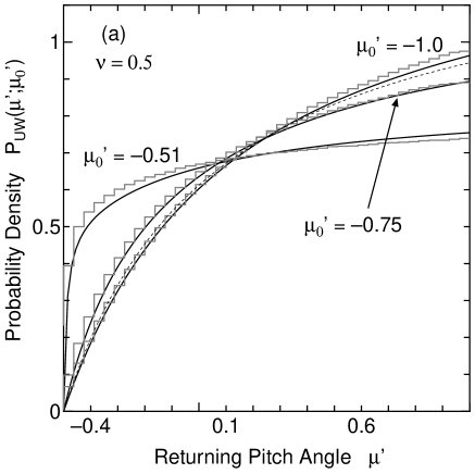
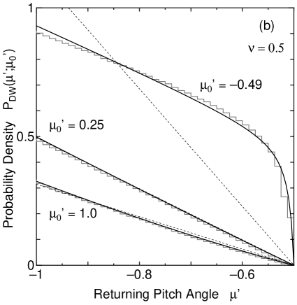
Figure 6: The probability densities of pitch angle at return for $\nu=0.5$ (a) ${P_{\rm UW}}(\mu^{\prime};\mu_{0}^{\prime})$ and (b) ${P_{\rm DW}}(\mu^{\prime};\mu_{0}^{\prime})$ for several values of the initial pitch angle $\mu_{0}^{\prime}$. Results of our approximation (solid curves), the multi-step approximation (dotted curves) and Monte Carlo simulation (grey histograms) are shown.

Fig. 6 shows the probability density of pitch angle at return ${P_{\rm UW}}(\mu_{0}^{\prime})$ in (a) and ${P_{\rm DW}}(\mu_{0}^{\prime})$ in (b) for $\nu=0.5$ and for several values of the initial pitch angle cosine $\mu_{0}^{\prime}$. Our approximation (solid curves) gives a fairly good fit to the Monte Carlo simulation (grey histograms) for all initial pitch angle cosine $\mu_{0}^{\prime}$. For small $\mu_{0}^{\prime}$, the fit deviates a little because the effects of the peak in ${n_{N}}(x)$ around $x=0$, which is ignored in our approximation, affect the probability density. The multi-step approximation (dotted curves) does not fit well when the initial mean free path ${\lambda^{*}_{0}}$ is small because effects of the return after only a few steps of scattering becomes important. But, for large ${\lambda^{*}_{0}}$ and for ${P_{\rm DW}}$, the multi-step approximation can fit to the Monte Carlo simulation.

The expression of the absorption probability $P_{\rm abs}(b)$ by our approximation is a little cumbersome and is presented in Appendix D. The absorption probability by the multi-step approximation is given by equation (70) together with equation (88). Fig. 7 presents $P_{\rm abs}(b)$ as a function of the initial position $b$ for $\nu=0.7$.

Figure 7: The absorption probability from $z$, $P_{\rm abs}(z)$, for $\nu=0.7$. Results of our approximation (solid curve), the multi-step approximation (dashed curve), and Monte Carlo simulation (filled circle) are represented. The results using the length $1/(3{\Gamma_{\rm f}}\nu)$ (lower dotted curve) or $1/(3\nu)$ (upper dotted curve) instead of ${L_{\rm D}}$ in the multi-step approximation are also shown as in Fig.2̃. The curve $1/(3\nu)$ also corresponds to the extrapolation of Peacock’s expression (his eq.(24)) to relativistic fluid speed.

The result of our approximation (solid curve) gives a good fit to the Monte Carlo results (filled circles) (small difference is in part caused by omitting the peak in ${n_{N}}(x)$). The multi-step approximation (dashed curve) deviates from the Monte Carlo results, but gives a correct scale length (${L_{\rm D}}$). This result directly confirms that the diffusion length for such large $\nu$ is given by our diffusion length ${L_{\rm D}}$. Results using the conventional diffusion length ${L_{\rm D0}}$ instead of ${L_{\rm D}}$ in the expression of the multi-step approximation (equation (70) and (65)) for two case as in Fig. 2 are also represented; lower dotted curve for $1/(3{\Gamma_{\rm f}}\nu)$ and upper dotted curve for $1/(3\nu)$). It should be noted that if we extrapolate the expression (24) in Peacock (1981), which was derived by adopting the diffusion approximation for particles in downstream of the shock front, to relativistic fluid speed in fluid frame and then transform it to the expression for the boundary rest frame, it turns out to correspond to the multi-step approximation (70) except that it has the scale length of return $1/(3\nu)$ (in our unit). These results do not give a satisfactory fit.

Fig. 8 presents the total return probability $P_{\rm R}(\mu_{0})$ from the downstream for mildly high $\nu$ ($\nu=1/3$) as a function of initial pitch angle cosine $\mu_{0}$, which is measured in the boundary rest frame.

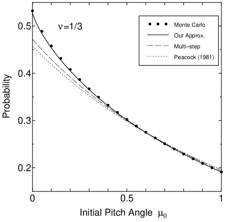
Figure 8: The total return probability $P_{\rm R}(\mu_{0})$ for $\nu=1/3$ from the downstream. Here, the initial pitch angle cosine $\mu_{0}$ is measured in the boundary rest frame. Results of our approximation (solid curve), the multi-step approximation (dashed curve), Peacock’s approximation (dotted curve) and Monte Carlo simulation (filled circle) are shown.

The results of our approximation (solid curve) excellently agree with the Monte Carlo simulation (filled circles). The dotted curve shows the approximate solution of Peacock [1981] (shown in his fig.2). The result of the multi-step approximation (dashed curve), which uses the correct length ${L_{\rm D}}$, is similar to Peacock’s one, but slightly better than it. These two diffusive approximations do not agree with the Monte Carlo results for small $\mu_{0}$. The reason is similar to that for ${P_{\rm UW}}$ and ${P_{\rm DW}}$; in diffusive approximations, effects of return after only a few steps of scattering are not accounted for. In general, for higher $\nu$ or smaller ${\lambda^{*}_{0}}$, such effects become important and these diffusive approximations become worse.

4.3 Density of scattering points

Here, we show the results of the density of the scattering points for the particles which cross the shock front with the pitch angle cosine $\mu_{0}^{\prime}$. Fig. 9 shows ${N_{-}}(z;\mu_{0}^{\prime})$ in (a) and ${N_{+}}(z;\mu_{0}^{\prime})$ in (b) calculated by the Monte Carlo simulation (histograms) for several values of the initial pitch angle $\mu_{0}^{\prime}$ along with our approximate solutions.

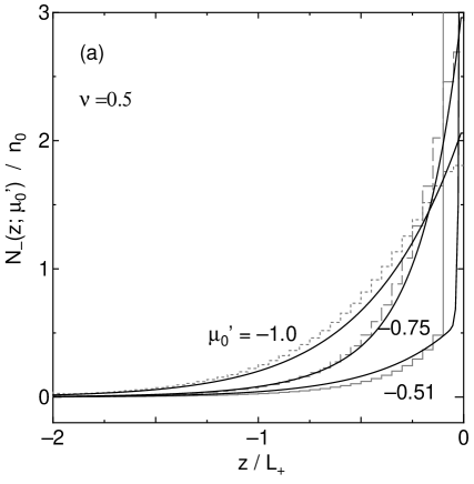
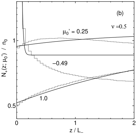
Figure 9: The density of the scattering points for particles which cross the boundary with the initial pitch angle $\mu_{0}^{\prime}$, (a) ${N_{-}}(z;\mu_{0}^{\prime})$ and (b) ${N_{+}}(z;\mu_{0}^{\prime})$. Results of our approximation (solid curves), and Monte Carlo simulation (histograms) are shown for $\nu=0.5$.

It is seen that our approximation (solid curves) coincides well with Monte Carlo simulation. But, a discrepancy is recognized for $z>0.3L_{-}$ in (b). Because the normalization conditions used in our approximation (the equation (39), (44)) employ only the information of finally absorbed particles and do not care about escaping particles to the far downstream, our approximation fails to give a good fit in a distant region where escaping particles dominate, while it gives a satisfactory fit in a near region where almost all the last scattering points exist. This also means that our approximation works well for absorbed particles, therefore the return probability densities themselves are represented by our approximations quite well as shown in Fig. 6 and Fig. 8.

Another important feature of ${N_{+}}$ and ${N_{-}}$ is that the density of the scattering points near the boundary depends on the initial pitch angle $\mu_{0}^{\prime}$. Here, we explain this feature for ${N_{+}}$ (that for ${N_{-}}$ is similar). Fig. 9 (b) shows that ${N_{+}}(z)$ increases when $z\rightarrow 0$ for small ${\lambda^{*}_{0}}$ but that it decreases when $z\rightarrow 0$ for large ${\lambda^{*}_{0}}$. This can be explained as already mentioned in Section 3; for small ${\lambda^{*}_{0}}$ the scattering point of few step particles are important, while for large ${\lambda^{*}_{0}}$ the effect of finite initial mean free path is important. In our approximate expression of (54), while $C_{1}^{\prime}$ is always positive, $C_{0}^{\prime}$ becomes negative for large ${\lambda^{*}_{0}}$, as shown in Fig. 10 (b). (This feature also appears for ${N_{-}}$, as shown in Fig. 10 (a).)

Figure 10: The coefficients in the expression of (a) ${N_{-}}(z;\mu_{0})$ and (b) ${N_{+}}(z;\mu_{0})$ for $\nu=0.5$ are shown as functions of the initial mean free path ${\lambda^{*}_{0}}$.

Because of this feature, when we average the return probability over an incoming particle distribution, the first term in (54), which denotes the non-diffusive effects, will become small enough compared with the diffusive term which is associated with $C_{1}^{\prime}$. Then, there appears a possibility to use the multi-step approximation to determine the averaged pitch angle distribution over all incident particles even if $\nu$ is large. The same consideration applies for ${N_{-}}$, too. As will be shown in the following section, at least for the isotropic large angle scattering model and for typical incoming $\mu_{0}^{\prime}$ distributions, this is actually the case. In practice, for this reason, we can use the multi-step approximation to determine the pitch angle distribution at the shock front for arbitrary shock speed as shown in the following section.

5 Application to the Shock
Acceleration

In this section, we apply the random walk theory developed so far to the shock acceleration and calculate the spectral index of the accelerated particles for the isotropic large angle scattering model described in the previous section. In the following, we consider the acceleration in parallel shocks where the fluid speed measured in the shock rest frame are uniform on each side of the shock front; ${V_{\rm u}}$ for the upstream and ${V_{\rm d}}$ for downstream respectively. We also consider only relativistic particles ($v^{\prime}\sim 1$, i.e., $\nu\sim{V_{\rm f}}$) because, in this case, the ratio $\nu$ does not change on each side of the shock front even if the particle gains energy in the process of multiple crossing at the shock front. In addition, for such particles, the Lorentz transformation of $\mu$ to $\mu^{\prime}$ becomes as simple as

$$\mu^{\prime}=\frac{\mu-{V_{\rm f}}}{1-\mu{V_{\rm f}}},\quad d\mu^{\prime}=\frac{1-{V_{\rm f}}^{2}}{(1-\mu{V_{\rm f}})^{2}}d\mu,$$ (90)

where $\mu$ is the pitch angle cosine measured in the shock rest frame. Hereafter, we use subscripts u, d or superscripts (u), (d) to indicate quantities in the upstream and downstream regions, respectively. The pitch angle cosine measured in the upstream fluid frame is denoted by $\mu^{\rm(u)}$ and that measured in the downstream fluid frame by $\mu^{\rm(d)}$.

In the following, we present the results only for two simple jump conditions $r={V_{\rm u}}/{V_{\rm d}}=4$ and $r=3V_{\rm s}^{2}$ (i.e., ${V_{\rm u}}{V_{\rm d}}=1/3$). But, since the results are expressed in terms of ${V_{\rm u}}$ and ${V_{\rm d}}$, they are applicable to any jump conditions. (Jump conditions for relativistic shocks are discussed in Blandford & McKee [1976], Peacock [1981], Appl & Camenzind [1988] and Heavens & Drury [1988].)

5.1 Method of determining the pitch angle
distribution at the shock front

The spectral index of the accelerated particles $\sigma$ is given by

$$\sigma=1-\frac{\ln({\langle P_{\rm R}\rangle})}{{{\langle\ln\delta\rangle}}}$$ (91)

where ${\langle P_{\rm R}\rangle}$ is the averaged return probability for the particles crossing the shock front toward downstream and ${\langle\ln\delta\rangle}$ is the logarithm of the energy gain factor (see Peacock 1981). (Here, $\langle\rangle$ denotes to average over the pitch angle distribution crossing the shock front.) ${\langle\ln\delta\rangle}$ is given as

$${\langle\ln\delta\rangle}=2\ln{\Gamma_{\rm rel}}+{\langle\ln\delta\rangle_{\rm ud}}+{\langle\ln\delta\rangle_{\rm du}},$$ (92)

where

$${\langle\ln\delta\rangle_{\rm ud}}:=\left<\ln(1+{V_{\rm rel}}\mu_{\rm ud}^{\rm(u)})\right>,$$ (93)

$${\langle\ln\delta\rangle_{\rm du}}:=\left<\ln(1-{V_{\rm rel}}\mu_{\rm du}^{\rm(d)})\right>$$ (94)

and ${V_{\rm rel}}$ is the relative velocity of the upstream fluid with respect to the downstream fluid,

$${V_{\rm rel}}=\frac{{V_{\rm u}}-{V_{\rm d}}}{1-{V_{\rm u}}{V_{\rm d}}},\qquad{\Gamma_{\rm rel}}:=\frac{1}{\sqrt{1-{V_{\rm rel}}^{2}}}.$$ (95)

If the dependences on $\mu^{\prime}$ and $v^{\prime}$ in $\lambda$ and $P_{\mu^{\prime}}$ are separable, these quantities are independent of the particle energy, i.e., $v^{\prime}$.

Introducing the normalized pitch angle distribution of particles crossing the shock front from upstream toward downstream by ${\Phi_{\rm ud}}(\mu^{\rm(u)})$, and that from downstream toward upstream by ${\Phi_{\rm du}}(\mu^{\rm(d)})$, i.e.,

$$\int_{-{\nu_{\rm u}}}^{1}{\Phi_{\rm ud}}(\mu^{\rm(u)})d\mu^{\rm(u)}=\int_{-1}^{-{\nu_{\rm d}}}{\Phi_{\rm du}}(\mu^{\rm(d)})d\mu^{\rm(d)}=1,$$

we can write relevant quantities as follows. Using $P_{\rm R}^{\rm(d)}(\mu^{\rm(d)})$ and ${\Phi_{\rm ud}}(\mu^{\rm(d)})$, ${\langle P_{\rm R}\rangle}$ is written as

$${\langle P_{\rm R}\rangle}=\int_{-{\nu_{\rm d}}}^{1}P_{\rm R}^{\rm(d)}(\mu^{\rm(d)}){\Phi_{\rm ud}}(\mu^{\rm(d)})d\mu^{\rm(d)}.$$ (96)

The logarithm of the energy gain factor is given by

$${\langle\ln\delta\rangle_{\rm ud}}=\int_{-{\nu_{\rm u}}}^{1}\!\ln(1+{V_{\rm rel}}\mu_{\rm ud}^{\rm(u)})\;\frac{P_{\rm R}^{\rm(d)}(\mu_{\rm ud}^{\rm(d)})}{{\langle P_{\rm R}\rangle}}{\Phi_{\rm ud}}(\mu_{\rm ud}^{\rm(u)})d\mu_{\rm ud}^{\rm(u)}$$ (97)

and

$${\langle\ln\delta\rangle_{\rm du}}=\int_{-1}^{-{\nu_{\rm d}}}\!\ln(1-{V_{\rm rel}}\mu_{\rm du}^{\rm(d)})\;{\Phi_{\rm du}}(\mu_{\rm du}^{\rm(d)})d\mu_{\rm du}^{\rm(d)}.$$ (98)

The factor $P_{\rm R}^{\rm(d)}(\mu_{\rm ud}^{\rm(d)})/{\langle P_{\rm R}\rangle}$ in equation (97) means that only particles which return again to the shock front are to be considered.

The pitch angle distribution ${\Phi_{\rm ud}}(\mu^{\rm(u)})$ and ${\Phi_{\rm du}}(\mu^{\rm(d)})$ in a steady state are determined as follows. If ${\Phi_{\rm ud}}(\mu^{\rm(u)})$ is known, ${\Phi_{\rm du}}(\mu^{\rm(d)})$ is determined by ${\Phi_{\rm ud}}(\mu^{\rm(u)})$,

$${\Phi_{\rm du}}(\mu^{\rm(d)})=\int_{-{\nu_{\rm u}}}^{1}\frac{P_{\rm DW}^{\rm(d)}(\mu^{\rm(d)};\mu_{0}^{\rm(d)})}{P_{\rm R}^{\rm(d)}(\mu_{0}^{\rm(d)})}{\Phi_{\rm ud}}(\mu_{0}^{\rm(u)})d\mu_{0}^{\rm(u)}.$$ (99)

On the other hand, ${\Phi_{\rm ud}}(\mu^{\rm(u)})$ is also determined by ${\Phi_{\rm du}}(\mu^{\rm(d)})$,

$${\Phi_{\rm ud}}(\mu^{\rm(u)})=\int_{-1}^{-{\nu_{\rm d}}}P_{\rm UW}^{\rm(u)}(\mu;\mu_{0}){\Phi_{\rm du}}(\mu_{0}^{\rm(d)})d\mu_{0}^{\rm(d)}.$$ (100)

Therefore, in a steady state, ${\Phi_{\rm du}}(\mu^{\rm(d)})$ satisfies an integral equation (a Fredholm equation of second kind)

$${\Phi_{\rm du}}(\mu^{\rm(d)})=\int_{-1}^{-{\nu_{\rm d}}}K(\mu^{\rm(d)};\mu_{0}^{\rm(d)}){\Phi_{\rm du}}(\mu_{0}^{\rm(d)})d\mu_{0}^{\rm(d)},$$ (101)

where the kernel of this integral equation is given by

$$K(\mu^{\rm(d)};\mu_{0}^{\rm(d)}):=\int_{-{\nu_{\rm u}}}^{1}\frac{P_{\rm DW}^{\rm(d)}(\mu^{\rm(d)};\mu_{1}^{\rm(d)})}{P_{\rm R}^{\rm(d)}(\mu_{1}^{\rm(d)})}P_{\rm UW}^{\rm(u)}(\mu_{1}^{\rm(u)};\mu_{0}^{\rm(u)})d\mu_{1}^{\rm(u)}.$$ (102)

This kernel denotes the probability density of the particle which crosses the shock front from downstream to upstream with $\mu_{0}^{\rm(d)}$ crosses the shock front again from downstream to upstream with $\mu^{\rm(d)}$ after one cycle. If ${\Phi_{\rm du}}(\mu^{\rm(d)})$ can be solved, ${\Phi_{\rm ud}}(\mu^{\rm(u)})$ is calculated through equation (100). Although in the above we have made the integral equation for ${\Phi_{\rm du}}(\mu^{\rm(d)})$, one can alternatively make the integral equation for ${\Phi_{\rm ud}}(\mu^{\rm(u)})$.

5.2 Approximate solution of the pitch angle
distribution at the shock front

It is generally difficult to solve the integral equation (101) analytically even if our approximation are used. Then, we numerically evaluate the kernel for our approximation. On the other hand, in the multi-step approximation, ${\Phi_{\rm ud}}(\mu)$ and ${\Phi_{\rm du}}(\mu)$ can be calculated analytically without solving the integral equation (101). Because the dependence of $P_{\rm DW}(\mu^{\prime};\mu^{\prime}_{0})$ in equation (63) are separable in $\mu^{\prime}$ and $\mu^{\prime}_{0}$ in this approximation, it becomes

$${\Phi_{\rm du}}(\mu^{\rm(d)})=\frac{P_{\mu^{\prime}}{{\lambda_{\rm d}}^{*}}}{{h_{-}}}.$$ (103)

Because $P_{\rm UW}(\mu^{\prime};\mu^{\prime}_{0})$ in equation (62) is independent of $\mu^{\prime}_{0}$, we obtain

$${\Phi_{\rm ud}}(\mu^{\rm(u)})=\frac{1}{{g_{+}}({L_{\rm D}})}\frac{P_{\mu^{\prime}}{\lambda^{*}}}{{\lambda^{*}}+{L_{\rm D}}}.$$ (104)

These results agree with the results obtained by Peacock(1981), but ${L_{\rm D}}$ was replaced by ${L_{\rm D0}}$ in equation (103).

Figure 11: The kernel of integral equation (100) for $V_{\rm s}=0.7$ and $r=3V_{\rm s}^{2}$. The numerical evaluation based on our approximation for $\mu_{0}=-0.01$ (solid curve), $-0.5$ (dashed curve) and $-1.0$ (dotted curve) are shown together with the result of the multi-step approximation (thin dotted curve). The results turn out to be almost independent of $\mu_{0}$ and all curves give similar results.

Fig. 11 shows the kernel of equation (101) for $V_{\rm s}=0.7$ and $r=3V_{\rm s}^{2}$. The numerical evaluation based on our approximation for $\mu_{0}=-0.01$ (solid curve), $-0.5$ (dashed curve) and $-1.0$ (dotted curve) together with that of the multi-step approximation are shown. It is seen that the kernel is almost independent of the initial pitch angle cosine $\mu_{0}$. The reason for this coincidence is considered to be due to compensation effects of several non-diffusive effects when averaged over the initial pitch angle as was mentioned in the previous section. Although this is partly due to our assumption of the isotropic large angle scattering, it is of a great importance in applications to the shock acceleration. Although the multi-step approximation is a poor approximation to the detailed particle transport, it can be a good approximation when we average over the pitch angle distribution. Thus, this result gives a justification for using the multi-step approximation even for relativistic shocks.

Fig. 12 presents the pitch angle distribution at the shock front in various frames for various shock velocities.

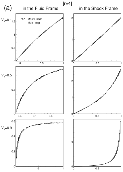
Figure 12: The pitch angle distribution of the particles crossing the shock front. Figure (a) refers to the particles crossing from upstream to downstream while figure (b) does those from downstream to upstream. The pitch angle distribution both in the fluid frame and the shock rest frame are shown. The results of the multi-step approximation (dotted curve) and the Monte Carlo simulation (solid histogram) are shown.

The results of the multi-step approximation (dotted curve) and the Monte Carlo simulation (solid histogram) are shown. As is seen, the results of the multi-step approximation agree quite well with the Monte Carlo results even for highly relativistic shocks. This is not surprising once we admit that the kernel is well approximated by the multi-step approximation. Thus, we have confirmed the point mentioned above that the multi-step approximation gives a good fit to the steady state pitch angle distribution at the shock for any shock speed. Also, it is to be noted that the assumptions used in Peacock (1981) are adequate for arbitrary shock speed if the correct diffusion length ${L_{\rm D}}$ is used in the downstream as in the multi-step approximation.

5.3 Approximate solution of the spectral index

Figure 13: The quantities associated with the shock acceleration, the spectral index $\sigma$, return probability ${\langle P_{\rm R}\rangle}$ from the downstream and the logarithm of energy gain factor ${\langle\ln\delta\rangle}$ for the compression ratio $r=4$ (a) and for the relativistic jump condition, ${V_{\rm u}}{V_{\rm d}}=1/3$ (b). Curves show the results of the multi-step approximation, while filled symbols show those of Monte Carlo simulation.

In the previous subsection, we have shown that the pitch angle distributions at the shock crossing ${\Phi_{\rm ud}}(\mu)$ and ${\Phi_{\rm du}}(\mu)$ can be well approximated by the multi-step approximation. Here, using this approximation, we show analytical expressions of the quantities associated with the shock acceleration, ${\langle P_{\rm R}\rangle}$, ${\langle\ln\delta\rangle}$ and $\sigma$, for the isotropic large angle scattering. First, using $P_{\rm R}(\mu_{0};{\nu_{\rm d}})$ (equation (64)) and ${\Phi_{\rm ud}}(\mu)$ by the multi-step approximation, ${\langle P_{\rm R}\rangle}$ is calculated as

$${\langle P_{\rm R}\rangle}=A^{\rm(d)}\cdot U({V_{\rm u}},{V_{\rm d}}),$$ (105)

where

$$U({V_{\rm u}},{V_{\rm d}}):=1+\frac{{\chi_{\rm d}}-1}{{\chi_{\rm u}}-{\chi_{\rm d}}}\left(1-\frac{\psi(\tilde{R})}{\psi(R_{+}^{\rm(u)})}\right),$$ (106)

with

$${\chi_{\rm u}}:=\frac{1}{{\Gamma_{\rm u}}^{2}({V_{\rm u}}-{V_{\rm d}})L_{\rm D}^{\rm(u)}},$$ (107)

$${\chi_{\rm d}}:=1+\frac{1}{{\Gamma_{\rm d}}^{2}({V_{\rm u}}-{V_{\rm d}})L_{\rm D}^{\rm(d)}},$$ (108)

$${\chi_{0}}:=\frac{{V_{\rm u}}-{V_{\rm d}}}{1-{V_{\rm u}}},\qquad{\chi_{1}}:=\frac{{V_{\rm u}}-{V_{\rm d}}}{1+{V_{\rm d}}},$$ (109)

$$\tilde{R}:={\chi_{0}}{\chi_{\rm d}}\qquad(R_{+}^{\rm(u)}={\chi_{0}}{\chi_{\rm u}}).$$ (110)

$\psi$ is defined in (89).

Then, the logarithm of the energy gain factor is given by

$${\langle\ln\delta\rangle_{\rm ud}}= \ln(1+{V_{\rm rel}})$$

$$+ \frac{\left(\frac{1}{{\chi_{\rm d}}}-\frac{1}{{\chi_{\rm u}}}\right)\psi({\chi_{0}})+({\chi_{\rm d}}-1)\Psi({\chi_{\rm d}})-({\chi_{\rm u}}-1)\Psi({\chi_{\rm u}})}{({\chi_{\rm d}}-1)\psi(\tilde{R})-({\chi_{\rm u}}-1)\psi(R_{+}^{\rm(u)})}$$ (111)

and

$${\langle\ln\delta\rangle_{\rm du}}=\ln(1+{V_{\rm rel}})+\frac{1}{2}\psi({\chi_{1}})-\frac{1}{2},$$ (112)

where

$$\Psi(x):=\frac{\ln(1+{\chi_{0}})\ln(x-1)+{\rm dilog}\left(\frac{1}{1-x}\right)-{\rm dilog}\left(\frac{1+{\chi_{0}}x}{1-x}\right)}{\frac{1}{2}({\chi_{0}}x)^{2}},$$ (113)

with Dilogarithm ${\rm dilog}\left(x\right)$ defined by (see Abramowitz & Stegun 1965)

$${\rm dilog}\left(x\right):=-\int_{1}^{x}\frac{\ln t}{t-1}dt.$$ (114)

Using these results, (91) gives the spectral index $\sigma$. In Fig. 13 (a) are presented the quantities associated with the shock accelerations as functions of shock speed $V_{\rm s}$ for the compression ratio $r=4$. In Fig. 13 (b) are shown the results for different jump condition (${V_{\rm u}}{V_{\rm d}}=1/3$). As is seen in these two figures, the result of the multi-step approximation excellently agree with the results of the Monte Carlo simulation even if shock speed becomes highly relativistic.

Fig. 14 presents the spectral index $\sigma$ as functions of the compression ratio $r$ similar to fig. 4 of Ellison et al. [1990].

Figure 14: The spectral index as functions of the compression ratio $r$ for various shock speed $V_{\rm s}$. The solid curves are our results based on the multi-step approximation, the dotted curves are the results of fitting formula of Ellison et al. (1990) and the filled circles are our Monte Carlo results. The dashed curve is the results of the conventional diffusion approximation, i.e., $\sigma=(r+2)/(r-1)$.

Our results (solid curves) basically coincide with their approximate expression (dashed curves; their equation(29)). Small discrepancy between these two results may be caused by the difference of the method to determine the spectral index $\sigma$; we calculate $\sigma$ using equation (91), while $\sigma$ was determined by fitting the calculated particle spectrum directly in Ellison et al. [1990].

6 Discussion

Although we have considered the particle acceleration in parallel shocks with the large angle scattering model, it is of some interest to discuss whether our formulation can be extended to other scattering regime.

Recently, the acceleration in ultra-relativistic shocks has attracted some attention in relation to the ultra-high-energy cosmic rays (UHECR). However, in such highly relativistic shocks, the large angle scattering model adopted here can not be used safely in a physical sense; because the residence time of particles in upstream is quite short (it is shorter than the gyro-period of particles), its point-like feature may lead to unsuitable results (Bednarz & Ostrowski 1996). This is also problematic for the pitch angle diffusion model based on the quasi-linear theory; because it assumes the resonance between the magnetohydrodynamical waves and particle gyro-motion, it requires time much longer than the gyro-period. Gallant & Achterberg (1999) proposed two deflection mechanisms of particles in upstream; regular deflection owing to the gyro-motion in uniform magnetic field, and ‘direction angle’ diffusion by randomly oriented small magnetic cells, where the direction angle is defined as the angle between the particle velocity and the shock normal. Gallant, Achterberg & Kirk (1999) and Kirk et al. (2000) calculated the spectral index using such direction angle diffusion model. Bednarz & Ostrowski (1998) also calculated the index adopting the small angle scattering model, which is approximately equivalent to the direction angle diffusion model in a mathematical sense. These works showed the spectral index $\sigma$ typically becomes $2.2$ for ultra-relativistic shock limit, while our large angle scattering model gives $\sigma\sim 1$. This index of 2.2 may be universal when the direction angle diffusion (or equivalent process) is proper for the scattering/deflection process in both upstream and downstream, though it is not yet settled whether the real scattering/deflection process during such quite short time can be treated well as a diffusion in direction angle.

Because our probability function based description of the shock acceleration described in Section 5.1 needs only two probability functions $P_{\rm UW}$ and $P_{\rm DW}$ to obtain the spectral index, it can be extended to include other scattering or deflection mechanisms if corresponding probability functions can be defined. For example, for the model of regular deflection in upstream the probability function $P_{\rm UW}$ can be defined and expressed in an analytical form under the condition that the direction of velocity perpendicular to the shock normal is randomly distributed at the shock crossing from downstream. Thus, if the large angle scattering model is adopted in downstream (assuming the Bohm diffusion), one can calculate the spectral index.

7 Conclusions

We have given a new formulation of the first order Fermi acceleration in shock waves with any shock speed in the point of view of the random walk of single particles suffering from large angle scattering. First, we have investigated the properties of particle trajectories in a moving medium. We showed that the problem could be formulated in terms of the random walk with absorbing boundaries based on the probability theory and derived an integral equation for the density of scattering points. By approximately solving it in an analytical form, we have given approximate analytic expressions for the probability density of pitch angle at return for particles which cross the shock front at a given pitch angle. We have confirmed that our approximate solutions agree with the Monte Carlo results quite well for the isotropic scattering. We have also shown that they are quite different from those based on the diffusion approximation for relativistic and mildly relativistic shocks. It is seen that the non-diffusive effects such as the return after only a few steps of scattering or the finite mean free path, which are not included in the diffusion approximation, are very important.

Using these results we have applied our formulation to the shock acceleration and compared our results with those in the literature such as ‘the relativistic diffusion approximation’, which was developed by Peacock [1981], together with the conventional diffusion approximation. We have found that the multi-step approximation, in which the effects of the return after only a few steps of scattering are neglected, gives a quite good fit to the Monte Carlo results on the pitch angle distributions at the shock crossing and the spectral index of accelerated particles. This is somewhat surprising because the multi-step approximation gives a poor fit to the Monte Carlo results when we fix the initial pitch angle at the shock crossing. One reason for this is considered that when averaging over the initial pitch angle, the effects of a few steps of return and the finite mean free path tend to cancel out and as a result the diffusive return term becomes dominant. Thus, our approach gives a theoretical base to use the multi-step approximation in the shock acceleration with any shock speed. We have also given a correct expression for the diffusive length scale for relativistic shocks, which equals to the scale lengths previously derived by Peacock [1981] and Kirk & Schneider (1988) for far upstream distribution in relativistic shocks, instead of a naive diffusion length based on the conventional diffusion equation.

Appendix A The relation between the density of scattering points and the physical number density

In order to consider the connection of the density of scattering points in random walk to the physical number density, let us introduce the concept of the staying time density. We define the staying time density $S(x)dx$ as the total staying time in the region between $x$ and $x+dx$ for the particle which is injected at the origin $x=0$ and absorbed eventually by one of the absorbing barriers. The total staying time in the non-absorbing region before absorption is clearly given by

$$\int_{-b}^{a}S(x)dx.$$

Then, the particle-averaged staying time density $\overline{S}(x)$ (i.e., the ensemble average of $S(x)$) is given as follows. Consider the contribution to the staying time of a particle between the successive scatterings. Since the probability of the particles to move beyond ${\Delta x}$ without scattering is ${\rm exp}(-|{\Delta x}|/{\lambda^{*}}(\mu^{\prime}))$ and since the staying time density is $|1/v\mu|$, the pitch angle averaged staying time density made by the particle during one step, $T({\Delta x})$, is given by

$$T({\Delta x})=\left\{\begin{array}[]{@{\,}ll}\displaystyle\int_{-\nu}^{1}P_{\mu^{\prime}}\frac{1}{v\mu}e^{-\frac{{\Delta x}}{{\lambda^{*}}(\mu^{\prime})}}d\mu^{\prime}&({\Delta x}>0)\\ \displaystyle\int_{-1}^{-\nu}P_{\mu^{\prime}}|\frac{1}{v\mu}|e^{\frac{{\Delta x}}{{\lambda^{*}}(\mu^{\prime})}}d\mu^{\prime}&({\Delta x}<0)\\ \end{array}\right.$$ (115)

where $v\mu$ is measured in the boundary rest frame. Using the probability density of the $m$-th scattering point $f_{m}(x)$, the staying time density made by the particles during the $m$-th step to $m+1$-th step is written as

$$\int_{-b}^{a}T(x-x^{\prime})f_{m}(x^{\prime})dx^{\prime}.$$

Therefore, summing up all steps from $m=0$ to $\infty$, the total staying time density is written as

$$\overline{S}(x)=\int_{-b}^{a}T(x-x^{\prime})n(x^{\prime})dx+T(x).$$

If we consider a steady state problem, in which particles are injected at the origin at a constant rate (with pitch angle distribution $P_{\mu^{\prime}}$), $\overline{S}(x)$ gives the physical number density for unit injection rate. These relations also have been used in the Monte Carlo simulations (e.g. Naito & Takahara 1995).

Appendix B Derivation of an alternative form of the integral equation

The problem of the random walk of single particles, which is discussed in Section 2, is equivalent to a steady state problem in which one particle is injected at the origin per one step. In the latter problem, $f_{m}(x)$ means the number density of scattering points of particles injected before $m$-steps and $n(x)$ correspond to the number density of scattering points made by all particles existing that time. Here, we consider the integral equation for $n(x)$ in this equivalent steady problem.

Let us consider the random walk of particles in steady state with no boundary but with imaginary boundaries at $x=a$ and $x=-b$. The number density of scattering points clearly equal to ${n_{N}}(x)$. Then, we can distinguish the particles that cross the boundaries at least once (‘passed particles’) from those that never crossed the boundaries (‘non-passed particles’). We write densities of scattering points of the former and latter particles as $n_{\rm pass}(x)$ and $n(x)$, respectively. This $n(x)$ obviously coincides with the density of scattering points of the random walk of single particle with the absorbing barriers at $x=a$ and $x=-b$. The sum of these two densities should be the solution for the no-boundary problem, ${n_{N}}(x)$,

$${n_{N}}(x)=n(x)+n_{\rm pass}(x).$$ (116)

Non-passed particles are injected at the origin steadily at one particle per step. On the other hand, passed particles are created when non-passed particles cross one of the imaginary boundaries and this can be regarded as the passed particles are injected at the first scattering point after they first cross the boundary. If we denote density of the first scattering point as $D(X)$, this is calculated by the distribution of non-passed particles $n(x)$ as,

$$D(X)=f(X)+\int_{-b}^{a}f(X-x^{\prime})n(x^{\prime})dx^{\prime}\quad(X>a\;\mbox{or}\;X<-b).$$ (117)

Each passed particle which is injected at each first scattering point $X_{\rm inj}$ makes the density of scattering point $n_{N}(x-X_{\rm inj})$. Thus, $n_{\rm pass}(x)$ is written as

$$n_{\rm pass}(x) = \int_{a}^{\infty}n_{N}(x-X)D(X)dX$$ (118)

$$+\int_{-\infty}^{-b}n_{N}(x-X)D(X)dX.$$

Using equation (116) and (118), we obtain

$$n(x) = n_{N}(x)-\int_{a}^{\infty}n_{N}(x-X)D(X)dX$$ (119)

$$-\int_{-\infty}^{-b}n_{N}(x-X)D(X)dX.$$

By the definition of $D(X)$,

$$\int_{a}^{\infty}n_{N}(x-X)D(X)dX=\int_{a}^{\infty}n_{N}(x-X)f(X)dX$$

$$+\int_{-b}^{a}n(x^{\prime})\int_{a}^{\infty}n_{N}(x-X)f(X-x^{\prime})dXdx^{\prime},$$ (120)

$$\int_{-\infty}^{-b}n_{N}(x-X)D(X)dX=\int_{-\infty}^{-b}n_{N}(x-X)f(X)dX$$

$$+\int_{-b}^{a}n(x^{\prime})\int_{-\infty}^{-b}n_{N}(x-X)f(X-x^{\prime})dXdx^{\prime}.$$ (121)

Thus, defining the kernel as

$$k(x,x^{\prime}) := \int_{a}^{\infty}n_{N}(x-X)f(X-x^{\prime})dX$$ (122)

$$+\int_{-\infty}^{-b}n_{N}(x-X)f(X-x^{\prime})dX,$$

we get a Fredholm integral equation of the second kind,

$$n(x)=n_{N}(x)-k(x,0)-\int_{-b}^{a}k(x,x^{\prime})n(x^{\prime})dx^{\prime}.$$ (123)

This provides an alternative form of the integral equation for $n(x)$.

Appendix C Derivation of integral condition for ${N_{+}}(x;\mu^{\prime}_{0})$

This is the case of $a\rightarrow\infty$. We first rewrite the Wald’s identity (21) as

$$\int_{-\infty}^{-b}e^{-{\theta_{0}}X}\int_{-b}^{\infty}f(X-x^{\prime})\left\{n(x^{\prime};\infty,b)+\delta(x^{\prime})\right\}dx^{\prime}dX=1.$$

This equation can be rewritten further as

$$\int_{-\infty}^{0}e^{-{\theta_{0}}X}\int_{0}^{\infty}f(X-x^{\prime})\left\{n(x^{\prime}-b;\infty,b)+\delta(x^{\prime}-b)\right\}dx^{\prime}dX$$

$$=e^{-{\theta_{0}}b}.$$ (124)

On the other hand, ${N_{+}}(x;\mu^{\prime}_{0})$ in the equation (41) can be rewritten as

$${N_{+}}(x;\mu^{\prime}_{0})=\frac{1}{{\lambda^{*}_{0}}}\int_{0}^{\infty}\left\{n(x^{\prime}-b;\infty,b)+\delta(x^{\prime}-b)\right\}e^{-\frac{b}{{\lambda^{*}_{0}}}}db.$$

Thus, combining these two, we obtain the condition to be satisfied for ${N_{+}}(x;\mu^{\prime}_{0})$:

$$\int_{-\infty}^{0}e^{-{\theta_{0}}X}\int_{0}^{\infty}f(X-x^{\prime}){N_{+}}(x^{\prime};\mu^{\prime}_{0})dx^{\prime}dX=\frac{1}{1+{\theta_{0}}{\lambda^{*}_{0}}}.$$ (125)

Using the representation of p.d.f. for large angle scattering model (9), this condition becomes equation (44).

Appendix D The absorption probability by our approximation

The absorption probability from initial position $b$, $P_{\rm abs}(b)$, by our approximation is calculated as follows.

$$P_{\rm abs}(b)=A^{\prime}e^{\frac{b}{{L_{\rm D}}}}+\eta(b)$$ (126)

where we define functions

$$\eta(b) := \frac{n_{0}{L_{\rm D}}^{2}}{2}\left\{(A\cdot(\frac{1}{n_{0}{L_{\rm D}}}+1+\rho)+\rho)\xi(b)\right.$$ (127)

$$+(\frac{1}{n_{0}{L_{\rm D}}}+A+\rho)R_{-}E_{2}(\frac{b}{L_{-}})+R_{-}^{2}E_{3}(\frac{b}{L_{-}})$$

$$\left.+\rho A\cdot(\frac{R_{-}}{1-R_{-}})e^{-\frac{b}{{L_{\rm D}}}}\cdot E_{2}(\frac{b}{L_{-}}-\frac{b}{{L_{\rm D}}})\right\},$$

$$\xi(b):=E_{1}(\frac{b}{L_{-}})-e^{-\frac{b}{{L_{\rm D}}}}E_{1}(\frac{b}{L_{-}}-\frac{b}{{L_{\rm D}}}).$$ (128)

and a constant

$$A^{\prime}:=n_{0}^{\prime}({h_{-}}+{g_{+}}({L_{\rm D}}){L_{\rm D}})+A\left\{1-\frac{n_{0}^{\prime}}{2}\frac{L_{-}^{2}}{1-R_{-}}\right\}.$$ (129)

References

- [1965] Abramowitz M., Stegun I.A., 1965, Handbook of Mathematical Functions. Dover, New York
- [1988] Appl S., Camenzind M., 1988, A&A, 206, 258
- [1977] Axford W.I., Leer E., Skadron G., 1977, Proc.15th Int. Cosmic Ray Conf.(Plovdiv), 11, 132
- [1978a] Bell A.R., 1978a, MNRAS, 182, 147
- [1987] Blandford R.D., Eichler D., 1987, Phys.Rep., 154, 1
- [1976] Blandford R.D., McKee C.F., 1976, Phys.Fluids, 19, 1130
- [1976] Blandford R.D., Ostriker J.P., 1978, ApJ, 221, L229
- [1996] Bednarz J., Ostrowski M., 1996, MNRAS, 283, 447
- [1998] Bednarz J., Ostrowski M., 1998, Phys.Rev.Lett., 80, 3911
- [1999] Berezhko E.G., Ellison D.C., 1999, ApJ, 526, 385
- [1965] Cox D.R., Miller H.D., 1965, The Theory of Stochastic Processes. Methuen, London
- [1983] Drury L.O’C., 1983, Rep.Prog.Phys, 46, 973
- [1990] Ellison D.C., Jones F.C., Reynolds S.P., 1990, ApJ, 360, 702
- [1996] Ellison D.C., Baring M.G., Jones F.C., 1996, ApJ, 473, 1029
- [1999] Gallant Y.A., Achterberg A., 1999, MNRAS, 305, L6
- [1999] Gallant Y.A., Achterberg A., Kirk J.G., 1999, A&AS, 138, 549
- [1988] Heavens A.F., Drury L.O’C., 1988, MNRAS, 235, 997
- [1999] Kirk J.G., Duffy P., 1999, J.Phys.G. Nucl.Part.Phys., 25, R163
- [2000] Kirk J.G., Guthmann W., Gallant Y.A., Achterberg A., 2000, ApJ, in press
- [1988] Kirk J.G., Schlickeiser R., Schneider P., 1988, ApJ, 328, 269
- [1987a] Kirk J.G., Schneider P., 1987a, ApJ, 315, 425
- [1988] Kirk J.G., Schneider P., 1988, A&A, 201, 177
- [1995] Koyama K., Petre R., Gotthelf E.V., Hawng U., Matsuura M., Ozaki M., Holt S.S., 1995, Nat, 378, 255
- [1977] Krymsky G.F., 1977, Soviet Phys.Dokl., 22, 327
- [1995] Malkov M.A., Völk H.J., 1995, A&A, 300, 605
- [1980] Melrose D.B., 1980, Plasma Astrophysics. Gordon and Breach, New York
- [1995] Naito T., Takahara F., 1995, MNRAS, 275, 1077
- [1991] Ostrowski M., 1991, MNRAS, 249, 551
- [1981] Peacock J.A., 1981, MNRAS, 196, 135