*

Abstract

Methods for compression and classification of galaxy spectra, which are useful for large galaxy redshift surveys (such as the SDSS, 2dF, 6dF and VIRMOS), are reviewed. In particular, we describe and contrast three methods: (i) Principal Component Analysis, (ii) Information Bottleneck, and (iii) Fisher Matrix. We show applications to 2dF galaxy spectra and to mock semi-analytic spectra, and we discuss how these methods can be used to study physical processes of galaxy formation, clustering and galaxy biasing in the new large redshift surveys.

1 Introduction

The classification of galaxies is commonly done using galaxy images, in the spirit of Hubble’s original diagram and its extensions (for a review see van den Bergh 1998). Galaxy spectra offer another way of classifying galaxies, which can be directly connected to the underlying astrophysics. Obviously, the relation between galaxy morphology and spectra also provides important insight into scenarios of galaxy formation. One motivation for studying galaxy spectra in a statistical way is that new redshift surveys (e.g. SDSS, 2dF, 6dF and VIRMOS) will soon produce millions of spectra. These large data sets can then be divided into subsets for studies of e.g. luminosity functions and clustering per spectral type (or a specific astrophysical parameter). Traditional methods of classifying galaxies “by eye” are clearly impractical in this context. The analysis and full exploitation of such data sets require well justified, automated and objective techniques to extract as much information as possible.

The concept of spectral classification goes back to Humason (1936) and Morgan & Mayall (1957). The end goal of galaxy classification is a better understanding of the physical origin of different populations and how they relate to one another. In order to interpret the results of any objective classification algorithm, we must relate the derived classes to the physical and observable galaxy properties that are intuitively familiar to astronomers. For example, important properties in determining the spectral characteristics of a galaxy are its mean stellar age and metallicity, or more generally its full star formation history. An assumed star formation history can be translated into a synthetic spectrum using models of stellar evolution (e.g., Bruzual & Charlot 1993, 1996; Fioc & Rocca-Volmerange 1997). Spectral features are also affected by dust reddening and nebular emission lines.

As with other Astronomical data, there are different approaches for analysing galaxy spectra. Conceptually, it is helpful to distinguish between three procedures:

• Data compression

• Classification

• Parameter estimation

The three might of course be related (e.g. classification can be done in a compressed space of the spectra, or in the space of astrophysical parameters estimated from the spectra).

Another distinction is between ’unsupervised’ methods (where the data ‘speak for themselves’, in a model-independent way) and ’supervised’ methods (based on training sets of models, or other data sets). The statistical methods can also be viewed as a ‘bridge’ between the data and the models, i.e. the same statistic can be applied to both data and models, as an effective way of comparing the two.

The outline of this review is as follows: In Section 2 we mention briefly two examples of data sets (2dF spectra and mock spectra), and then in Sections 3,4 and 5 we present three methods: PCA, the Information Bottleneck and Fisher Matrix. In Section 6 we compare and contrast these and some other methods, and suggest directions for future work.

2 Spectral Ensembles

We mention above the exponential growth of data of galaxy spectra. Here we present two specific ‘proto-types’ of real and mock data, which are used later to illustrate the methods.

2.1 Observed Spectra from the 2dF Survey

The 2dF Galaxy Redshift Survey (2dFGRS; Colless 1998, Folkes et al. 1999) is a major new redshift survey utilising the 2dF multi-fibre spectrograph on the Anglo-Australian Telescope (AAT). The observational goal of the survey is to obtain high quality spectra and redshifts for 250,000 galaxies to an extinction-corrected limit of $b_{J}$=19.45. The survey will eventually cover approximately 2000 sq deg, made up of two continuous declination strips plus 100 random $2^{\circ}$-diameter fields. Over 135,000 galaxy spectra have been obtained as of October 2000. The spectral scale is 4.3Å  per pixel and the FWHM resolution is about 2 pixels. Galaxies at the survey limit of $b_{J}$=19.45 have a median S/N of $\sim 14$, which is more than adequate for measuring redshifts and permits reliable spectral types to be determined.

Here we use a subset of 2dF galaxy spectra, previously used in the analysis of Folkes et al. (1999). The spectra are given in terms of photon counts (as opposed to energy flux). The spectra were de-redshifted to their rest frame and re-sampled to a uniform spectral scale with 4Å bins, from 3700Å to 6650Å. The sample contains 5869 galaxies, each described by 738 spectral bins. Throughout this paper, we refer to this ensemble as the “2dF sample”. We corrected each spectrum by dividing it by a global system response function (Folkes et al. 1999). However, it is known that due to various problems related to the telescope optics, the seeing, the fibre aperture etc. the above correction is not perfect. In fact, each spectrum should be corrected by an individual response function (work in progress).

We note that another selection effect is due to the fixed diameter of the 2dF fibre (of 2 arcsec, which corresponds in an Einstein-de Sitter universe to $\sim 2.5h^{-1}$ kpc at the survey median redshift of 0.1). The observed spectrum is hence sensitive to the fraction of bulge versus disk which is in the fibre beam, and hence it it affected by the distance to the galaxy (see Kochanek et al. 2000). However, other effects such as poor seeing reduce this effect. The ‘aperture bias’ is also likely to be less dramatic if the spectral diagnostic used is continuum-based (rather than a diagnostic which is sensitive to emission lines that originate from star-forming regions). We also note that in a flux limited sample, distant objects are more intrinsically luminous, and this effect slightly biases distant populations towards early-type.

2.2 Model Spectra from Semi-Analytic Hierarchical Merger Models

In one example of applying PCA to mock spectra (Ronen, Aragon-Salamance & Lahav 1999), the star formation history was parameterized as a simple single burst or an exponentially decreasing star formation rate. However, the construction of the ensemble of galaxy spectra was done in an ad-hoc manner. An improvement to this approach is to use a cosmologically motivated ensemble of synthetic galaxies, with realistic star formation histories. These histories are determined by the physical processes of galaxy formation in the context of hierarchical structure formation. Semi-analytic models have the advantage of being computationally efficient, while being set within the fashionable hierarchical framework of the Cold Dark Matter (CDM) scenario of structure formation. In addition to model spectra, this approach provides many physical properties of the galaxies, such as the mean stellar age and metallicity, size, mass, bulge-to-disk ratio, etc. This allows us to determine how effectively a given method can extract this type of information from the spectra, which are determined in a self-consistent way. In Slonim et al. (2000; herafter SSTL) we describe a “mock 2dF” sample, produced using the semi-analytic model developed by Somerville (1997) and Somerville & Primack (1999), which has been shown to give good agreement with many properties of local and high-redshift galaxies. The “mock 2dF” given in SSTL has $2611$ model galaxies with the same magnitude limit, wavelength coverage and spectral resolution, and redshift range as the 2dF survey. The effects of the response function of the fibres, aperture effects, and systematic errors related to the placement of fibres were neglected.

The star formation histories were convolved with stellar population models to calculate magnitudes and colors and produce model spectra. SSTL used the multi-metallicity GISSEL models (Bruzual & Charlot, in preparation) with a Salpeter IMF to calculate the stellar part of the spectra. Emission lines from ionized $H_{\rm II}$ regions were added using the empirical library included in the PEGASE models (Fioc & Rocca-Volmerange 1997). Dust extinction was included using an approach similar to that of Guiderdoni & Rocca-Volmerange (1987). Poisson noise was added, based on an empirical relation from the 2dF data.

Figure 1 shows the mean spectrum for the 2dF and mock+noise catalogues, obtained by simply averaging the photon counts in each wavelength bin for all the galaxies in the ensemble. The mean spectra for the observed and mock catalogues are seen to be similar. The magnitude limit that we have chosen is such that our ensembles are dominated by fairly bright, moderately star-forming spiral galaxies, and the mean spectra show familiar features such as the 4000 Å break, the Balmer series, and metal lines such as O_II and O_III.

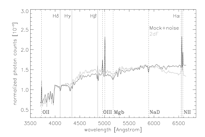
Figure 1: Photon counts (sum normalised to unity) as a function of wavelength, averaged over the entire catalogues of 2dF and mock+noise spectra. Note the familiar spectral features such as the Balmer break at 4000 Å, the Balmer series (marked with vertical grey lines), and metal lines such as O, Mg, Na, and N (marked by dotted lines). One can see that the 2dF spectrum appears to bend downwards relative to the models towards both ends of the wavelength range. This may be due to an inaccurate correction for the response function. (Figure from SSTL 2000.)

3 Principal Component Analysis (PCA)

PCA has previously been applied to data compression and classification of spectral data of stars (e.g. Murtagh & Heck 1987; Bailer-Jones et al. 1997), QSO (e.g. Francis et al. 1992) and galaxies (e.g. Connolly et al. 1995a; Folkes, Lahav & Maddox 1996; Sodre & Cuevas 1997; Galaz & de Lapparent 1997; Bromley et al. 1998; Glazebrook, Offer & Deeley 1998; Ronen et al. 1999; Folkes et al. 1999). While PCA operates as an efficient data compression algorithm, it is purely linear, based only on the variance of the distribution. PCA on its own does not provide a rule for how to divide the galaxies into classes .

A spectrum, like any other vector, can be thought of as a point in a high-dimensional parameter space. One may wish for a more compact description of the data. By identifying the linear combination of input parameters with maximum variance, PCA finds the principal components that can be most effectively used to characterise the inputs.

The formulation of standard PCA is as follows. Consider a set of $N_{G}$ galaxies ($i=1,N_{G}$), each with $N_{S}$ spectral bins ($j=1,N_{S}$). If $r_{ij}$ are the original measurements of these parameters for these objects, then mean subtracted quantities can be constructed,

$$X_{ij}=r_{ij}-{\bar{r}_{j}}\ ,$$ (1)

where ${\bar{r}_{j}}={1\over N_{G}}\sum_{i=1}^{N_{G}}r_{ij}$ is the mean. The covariance matrix for these quantities is given by

$$C_{jk}={1\over N_{G}}\sum_{i=1}^{N_{G}}X_{ij}X_{ik}\hskip 14.22636pt1\leq j\leq N_{S}\hskip 14.22636pt1\leq k\leq N_{S}\ .$$ (2)

It can be shown that the axis (i.e, direction in vector space) along which the variance is maximal is the eigenvector ${\bf e_{1}}$ of the matrix equation

$$C{\bf e_{1}}=\lambda_{1}{\bf e_{1}}\ ,$$ (3)

where $\lambda_{1}$ is the largest eigenvalue (in fact the variance along the new axis). The other principal axes and eigenvectors obey similar equations. It is convenient to sort them in decreasing order (ordering by variance), and to quantify the fractional variance by $\lambda_{\alpha}/\sum_{\alpha}\lambda_{\alpha}$. The matrix of all the eigenvectors forms a new set of orthogonal axes which are ideally suited to an efficient description of the data set using a truncated eigenvector matrix employing only the first $P$ eigenvectors

$$U_{P}=\{e_{jk}\}\hskip 28.45274pt1\leq k\leq P\hskip 28.45274pt1\leq j\leq N_{S}\ ,$$ (4)

where $e_{jk}$ is the $j$th component of the $k$th eigenvector. The first few eigenvalues account for most of the variation in the data, and the higher eigenvectors contain mostly the noise (e.g. Folkes, Lahav & Maddox 1996). The projection vector ${\bf z}$ onto the $M=N_{S}$ principal components can be found from (here ${\bf x}$ and ${\bf z}$ are row vectors):

$${\bf z}={\bf x}U_{M}\ .$$ (5)

Multiplying by the inverse, the spectrum is given by

$${\bf x}={\bf z}{U_{M}}^{-1}={\bf z}{U_{M}}^{t}\ ,$$ (6)

since $U_{M}$ is an orthogonal matrix by definition. However, using only $P$ principal components, the reconstructed spectrum would be

$${\bf x}_{rec}={\bf z}{U_{P}}^{t}\ ,$$ (7)

which is an approximation to the true spectrum.

The eigenvectors onto which we project the spectra can be viewed as ‘optimal filters’ of the spectra, in analogy with other spectral diagnostics such as colour filter or spectral index. Finally, we note that there is some freedom of choice as to whether to represent a spectrum as a vector of fluxes or of photon counts. The decision will affect the resulting principal components, as a representation by fluxes will give more weight to the blue end of a spectrum than a representation by photon counts. Figure 2 shows the mean spectrum for the 2dF sample, the first and second eigenvectors in the 2dF and the mock samples, and the $(pc1,pc2)$ projections for the 2dF sample. Given the observational uncertainties described above and the astrophysical unknowns, the similarity of the real and mock eigenvectors is quite remarkable.

Figure 2: The mean spectrum of the 2dF sample the first and second eigenvectors (with associated variances of 50% and 11 %, respectively), and the projections into the $(pc1,pc2)$ space. For comparison we show the two eigenvectors of the mock sample.

4 The Information Bottleneck (IB)

Here we summarize the Information Bottleneck (IB) method of Slonim et al. 2000 (SSTL), and suggest some extensions. The IB approach is based on the method of Tishby, Pereira & Bialek (1999), which has been successfully applied to the analysis of neural codes, linguistic data and classification of text documents. In the latter case, for example, one may see an analogy between an ensemble of galaxy spectra and a set of text documents. The words in a document play a similar role to the wavelengths of photons in a galaxy spectrum, i.e. the frequency of occurrence of a given word in a given document is equivalent to the number of photon counts at a given wavelength in a given galaxy spectrum. In both cases, the specific patterns of these occurrences may be used in order to classify the galaxies or documents.

4.1 “Euclidean” Classification

We may gain some intuition into the IB method by first considering standard clustering algorithms. Suppose we start from Bayes’ theorem, where the probability for a class ${c}$ for a given galaxy ${g}$ is

$$p({c}|{g})\propto p({c})\;p({g}|{c})\;,$$ (8)

and $p(c)$ is the prior probability for class $c$. As a simple ad-hoc example, we can take the conditional probability $p({g}|{c})$ to be a Gaussian distribution with variance $\sigma^{2}$

$$p({g}|{c})=\frac{1}{\sqrt{2\pi}\sigma}\;\exp(-\frac{1}{2\sigma^{2}}D_{E}^{2})\;,$$ (9)

with the Euclidean distance $D_{E}$:

$$D_{E}=\sqrt{\sum_{\lambda}[p({\lambda}|c)-p({\lambda}|g)]^{2}}\;.$$ (10)

The variance $\sigma^{2}$ may be due cosmic scatter as well as noise. Hence $\sigma$ can be viewed as the ‘resolution’ or the effective ‘size’ of the class in the high-dimensional representation space. We note that the Euclidean distance is commonly used in supervised spectral classification using ‘template matching’ (e.g. Connolly et al. 1995; Benitez 2000), in which galaxies are classified by matching the observed spectrum with a template obtained either from a model or from an observed standard galaxy. By comparing the IB method with this “Euclidean algorithm”, we find that the IB approach yields better class boundaries and preserves more information for a given number of classes.

4.2 Mutual Information and the Bottleneck

In the following we denote the set of galaxies by ${G}$ and the array of wavelength bins by ${\Lambda}$. We view the ensemble of spectra as a joint distribution $p({g},{\lambda})$, which is the joint probability of observing a photon from galaxy ${g}\in{G}$ at a wavelength ${\lambda}\in{\Lambda}$. We normalize the total photon counts in each spectrum (galaxy) to unity, i.e. we take the prior probability $p({g})$ of observing a galaxy ${g}$ to be uniform: $p({g})=\frac{1}{N_{G}}$, where $N_{G}$ is the number of galaxies in this sample ${G}$. This view of the ensemble of spectra as a conditional probability distribution function enables us to undertake the information theory-based approach that we describe in this section. Our goal is to group the galaxies into classes that preserve some objectively defined spectral properties. Ideally, we would like to make the number of classes as small as possible (i.e. to find the ‘least complex’ representation) with minimal loss of the ‘important’ or ‘relevant’ information. In order to do this objectively, we need to define formal measures of ‘complexity’ and ‘relevant information’.

The prior probability for a specific class ${c}$ is given by

$$p({c})=\sum_{{g}}p({g})p({c}|{g})~{}.$$ (11)

We can also write down:

$$p({\lambda}|{c})=\sum_{{g}}p({\lambda}|{g})p({g}|{c})~{},$$ (12)

where $p({\lambda}|{c})$ can be clearly interpreted as the spectral density associated with the class ${c}$.

The mutual information between two variables can be shown (see e.g. Cover & Thomas 1991) to be given by the amount of uncertainty in one variable that is removed by the knowledge of the other one, for example for the pair $({G},{\Lambda})$:

$$I({G};{\Lambda})=\sum_{{g},{\lambda}}p({g},{\lambda})\log\frac{p({g},{\lambda})}{p({g})p({\lambda})}~{}=\sum_{{g},{\lambda}}p({g})p({\lambda}|{g})\log\frac{p({\lambda}|{g})}{p({\lambda})}~{},$$ (13)

using $p({g},{\lambda})=p({g})p({\lambda}|{g})$. It is easy to see that $I({G};{\Lambda})$ is symmetric and non-negative, and is equal to zero if and only if ${g}$ and ${\lambda}$ are independent. Similarly we can define the mutual information between a set of galaxy classes ${C}$ and the spectral wavelengths ${\Lambda}$, $I({C};{\Lambda})=\sum_{{c},{\lambda}}p({c})p({\lambda}|{c})\log\frac{p({\lambda}|{c})}{p({\lambda})}$, and the mutual information between the classes and the galaxies $I({C};{G})=\sum_{{c},{g}}p({g})p({c}|{g})\log\frac{p({c}|{g})}{p({c})}$.

A basic theorem in information theory, known as data processing inequality, states that no manipulation of the data can increase the amount of (mutual) information given in that data. Specifically this means that by grouping the galaxies into classes one can only lose information about the spectra, i.e. $I({C};{\Lambda})\leq I({G};{\Lambda})$.

The problem can be formulated as follows: how do we find classes of galaxies that maximize $I({C};{\Lambda})$, under a constraint on $I({C};{G})$? In effect we pass the information that ${G}$ provides about ${\Lambda}$ through a “bottleneck” formed by the classes in ${C}$. The classes ${C}$ are forced to extract the relevant information between ${G}$ and ${\Lambda}$. Hence the name information bottleneck method .

Under this formulation, the optimal classification is given by maximizing the functional

$${\cal L}[p({c}|{g})]=I({C};{\Lambda})-\beta^{-1}I({C};{G}),$$ (14)

where ${\beta^{-1}}$ is the Lagrange multiplier attached to the complexity constraint. For $\beta\rightarrow 0$ our classification is as non-informative (and compact) as possible — all galaxies are assigned to a single class. On the other hand, as $\beta\rightarrow\infty$ the representation becomes arbitrarily detailed. By varying the single parameter $\beta$, one can explore the tradeoff between the preserved meaningful information, $I({C};{\Lambda})$, and the compression level, $I({C};G)$, at various resolutions.

The optimal assignment that maximizes Eq. (14) satisfies the equation

$$p({c}|{g})={{p({c})}\over Z({g},\beta)}\exp(-\beta D_{KL})~{},$$ (15)

where $Z(g,\beta)$ is the common normalisation (partition) function . The value in the exponent can be considered the relevant “distortion function” between the class and the galaxy spectrum. It turns out to be the familiar cross-entropy (also known as the ‘Kullback-Leibler divergence’, e.g. Cover & Thomas 1991), defined by

$$D_{KL}\left[p({\lambda}|{g})\|p({\lambda}|{c})\right]=\sum_{{\lambda}}p({\lambda}|{g})\log{{p({\lambda}|{g})}\over{p({\lambda}|{c})}}~{}.$$ (16)

Note that Eqs. (11, 12, 15) must be solved together in a self-consistent manner. We can also see now the analogy with the ‘Euclidean equations’ (section 4.1), i.e. between $D_{KL}$ and $D_{E}$, and between $\beta$ and $\sigma^{2}$. The IB approach is obviously far more ‘principled’.

4.3 The Agglomerative IB Algorithm

In practice we actually used a special case of the algorithm, based on a bottom-up merging process. This algorithm generates “hard” classifications, i.e. every galaxy ${g}\in{G}$ is assigned to exactly one class ${c}\in{C}$. Therefore, the membership probabilities $p({c}|{g})$ may only have values of $0$ or $1$. Thus, a specific class ${c}$ is defined by the following equations, which are actually the “hard” limit $\beta\rightarrow\infty$ of the general self-consistent Eqs. (11, 12, 15) presented previously,

$$\left\{\begin{array}[]{l}p({c})=\sum_{{g}\in{c}}{p({g})}\\ \\ p({\lambda}|{c})=\frac{1}{p({c})}\sum_{{g}\in{c}}p({\lambda}|{g})p({g})\\ \\ p({c}|{g})=\left\{\begin{array}[]{ll}1&\mbox{if ${g}\in{c}$}\\ 0&\mbox{otherwise}\end{array}\right.\\ \end{array}\right.$$ (17)

where for the second equation we used Bayes’ theorem, $p({g}|{c})=\frac{1}{p({c})}p({c}|{g})p({g})$.

The algorithm starts with the trivial solution, where ${C}\equiv{G}$ and every galaxy is in a class of its own. In every step two classes are merged such that the mutual information $I({C};{\Lambda})$ is maximally preserved. Note that this algorithm naturally finds a classification for any desired number of classes with no need to take into account the theoretical constraint via $\beta$ (Eq. 14). This is due to the fact that the agglomerative procedure contains an inherent algorithmic compression constraint, i.e. the merging process (for more details see SSTL).

4.4 IB Classification Results

We now apply the IB algorithm to both the 2dF and the mock data. Recall that our algorithm begins with one class per galaxy, and groups galaxies so as to minimize the loss of information at each stage. Figure 3 shows how the information content of the ensemble of galaxy spectra decreases as the galaxies are grouped together and the number of classes decreases. In the left panel, we show the ‘normalized’ information content $I({C};{\Lambda})/I({G};{\Lambda})$ as a function of the reduced complexity $N_{C}/N_{G}$, where $N_{G}$ is the number of galaxies in the ensemble and $N_{C}$ is the number of classes. Remarkably, we find that if we keep about five classes, about $85$ and $75$ percent of the information is preserved for the mock and mock+noise simulations, respectively. This indicates that the wavelength bins in the model galaxy spectra are highly correlated. In contrast with the mock samples, for the 2dF catalogue, only about $50$ percent of the information is preserved by five classes . This discrepancy may be partially due to the influence on the real spectra of more complicated physics than what is included in our simple models. It could also be due to systematic observational errors mentioned earlier.

Figure 3: Left Panel: The fractional information measure ($I({C};{\Lambda})/I({G};{\Lambda})$) vs. the fractional number of classes ($N_{C}/N_{G}$). The crosses mark the points corresponding to five classes, used in the remainder of this paper. Right Panel: The ‘absolute’ information content $I({C};{\Lambda})$ as a function of the number of classes $N_{C}$. (From SSTL 2000.)

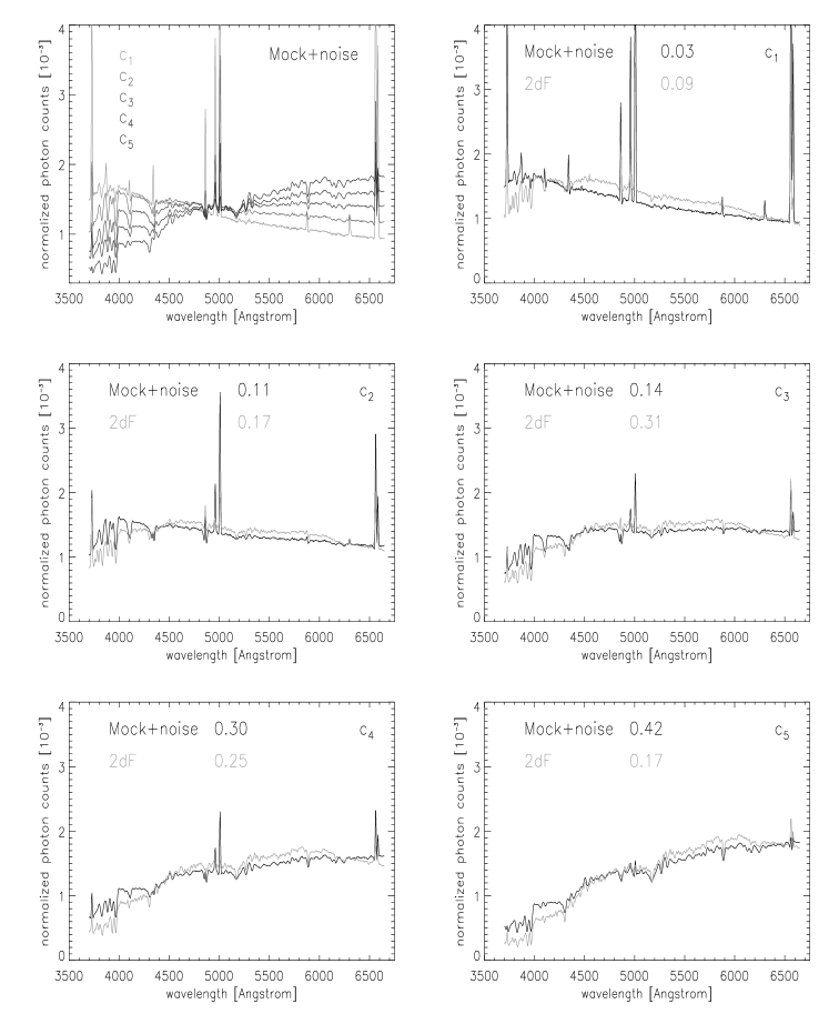
Figure 4: Mean spectra of the five IB classes for the 2dF and mock+noise catalogues. The fraction $p(c_{j})$ of galaxies that are members of each class $c_{j}$ is indicated. The matching between the classes obtained for 2dF and the mock catalogue was determined by minimizing the average ‘distance’ between the pairs. (From SSTL 2000.)

We now present the results obtained for five classes. Figure 4 shows the representative spectra for these five classes for both the 2dF and mock+noise catalogues. The corresponding five spectra for the noise-free mock data were very similar to the mock+noise spectra shown. We ‘matched’ each of the classes obtained for the 2dF data with one from the mock+noise data by minimizing the average ‘distance’ between the pairs. The classes are then ordered by their mean $B-V$ colour. Note that the five classes produced by the algorithm appear similar for both catalogues — there was certainly no guarantee that this would be the case.

It is also interesting to examine the relative fractions of galaxies in each class, $p(c)$, for the observed and mock catalogues. These values are given on the appropriate panels of Figure 4. More generally, we can see that the algorithm is sensitive to the overall slope (or colour) of the spectrum, and also to the strength of the emission lines. The classes clearly preserve the familiar physical correlation of colour and emission line strength; the five classes form a sequence from ${c}_{1}$, which has a blue continuum with strong emission lines, to ${c}_{5}$, with red continuum with no emission lines. It is interesting to compare the mean spectrum of ${c}_{1}$ with the spectrum of the Sm/Irr galaxy NGC449, and ${c}_{5}$ with the Sa galaxy NGC775 from Figure 2a of Kennicutt (1992). Apparently, the ${c}_{1}$ class corresponds to late type galaxies (Sm/Irr) and ${c}_{5}$ to early types (Sa-E). In order to gain a better understanding of the IB classes, we also use the noise-free mock catalogue and investigate the physical properties of the galaxies in each class as given by the same models that we use to produce the spectra. The strongest trend is of $B-V$ colour and present-to-past-averaged star formation rate (see Figure 5 in SSTL).

4.5 Comparison of IB with PCA

It is interesting to see where the IB classes reside in the space of the PCA projections. The 5 IB classes form fairly well-separated “clumps” in PC1-PC2 space, and that to a first approximation, the IB classification is along PC1 (see Figure 14 in SSTL). The PCA-space of the IB clumps looks quite different from the partitioning (based on training sets) given in Folkes et al. (1999), which was mainly based on emission and absorption lines (rather than on the continuum). It has been shown (Ronen et al. 1999) that PC1 and PC2 are correlated with colour and emission line strength, and the sequence from ${c}_{1}$-${c}_{5}$ is again sensible in this context.

4.6 Extensions of the IB Approach

4.6.1 Unsupervised ‘Wavelength Grouping’

We can ask a different question using the IB tool: What set ${C}_{{\Lambda}}$ of wavelength combinations (‘filters’) are the best indicators of the galaxy identity ?

This can be done by simply interchanging ${g}$ and ${\lambda}$ in eq.  17:

$$\left\{\begin{array}[]{l}p({c}_{{\Lambda}})=\sum_{{\lambda}\in{c}_{{\Lambda}}}{p({\lambda})}\\ \\ p({g}|{c}_{{\Lambda}})=\frac{1}{p({c}_{{\Lambda}})}\sum_{{\lambda}\in{c}_{{\Lambda}}}p({g}|{\lambda})p({\lambda})\\ \\ p({c}_{{\Lambda}}|{\lambda})=\left\{\begin{array}[]{ll}1&\mbox{if ${\lambda}\in{c}_{{\Lambda}}$}\\ 0&\mbox{otherwise}\end{array}\right.\\ \end{array}\right.$$ (18)

One difference is that while we have taken $p({g})=1/N_{G}$, here $p({\lambda})$ is the mean spectrum of the sample. Our preliminary results indicate that 10 combinations of spectral lines retain 68 % of the information in the case of the 2dF sample, and 96 % for the mock sample (Slonim et al., in preparation).

4.6.2 Supervised ‘Wavelength Grouping’

Another approach is to group wavelengths which are the most informative about physical parameters, e.g. age, star formation rate, etc. Commonly this question is answered by a more intuitive way, e.g. by extracting the H$\alpha$ line as an indicator of star formation rate.

This is in fact a formal principled solution to the fundamental question on the best spectral diagnostics of physical parameters. For a physical parameter of interest $a$ the relevant set of equations is now:

$$\left\{\begin{array}[]{l}p({c}_{{\Lambda}})=\sum_{{\lambda}\in{c}_{{\Lambda}}}{p({\lambda})}\\ \\ p(a|{c}_{{\Lambda}})=\frac{1}{p({c}_{{\Lambda}})}\sum_{{\lambda}\in{c}_{{\Lambda}}}p(a|{\lambda})p({\lambda})\\ \\ p({c}_{{\Lambda}}|{\lambda})=\left\{\begin{array}[]{ll}1&\mbox{if ${\lambda}\in{c}_{{\Lambda}}$}\\ 0&\mbox{otherwise}\end{array}\right.\\ \end{array}\right.$$ (19)

We shall show elsewhere the implementation of these ‘wavelength grouping’ algorithms. The next section is another approach for relating spectral features to physical parameters.

5 Maximum Likelihood and the Fisher Matrix (FM) Approach

In the case that an underlying astrophysical model for the spectrum is assumed, one may find the best fit parameters, by Maximum Likelihood. Heavens, Jimenez & Lahav (HJL 2000) presented a Maximum Likelihood method with radical linear compression of the datasets. In the case that the noise in the data is independent of the parameters, one can form $M$ linear combinations of the data which contain as much information about all the parameters as the entire dataset, in the sense that the Fisher information matrices are identical; i.e. the method is lossless. When the noise is dependent on the parameters (as in the case of galaxy spectra), the method is not precisely lossless, but the errors increase by a very modest factor. This data compression offers the possibility of a large increase in the speed of determining physical parameters. This is an important consideration as datasets of galaxy spectra reach $\sim 10^{6}$ in size, and the complexity of model spectra increases. In addition to this practical advantage, the compressed data may offer a classification scheme for galaxy spectra which is based rather directly on physical processes.

5.1 The FM Compression Method

Here we represent a spectrum as a vector ${\bf x}_{i}$, $i=1,\ldots,N_{S}$ (e.g. a set of fluxes at different wavelengths). These measurements include a signal part, which we denote by $\mu$, and noise, ${\bf n}$:

$${\bf x}=\mbox{\boldmath$\mu$}+{\bf n}$$ (20)

Assuming the noise has zero mean, $\langle{\bf x}\rangle=\mbox{\boldmath$\mu$}$. The signal will depend on a set of physical parameters $\{\theta_{\alpha}\}$, which we wish to determine. For galaxy spectra, the parameters may be, for example, age, magnitude of source, metallicity and some parameters describing the star formation history. Thus, $\mu$ is a noise-free spectrum of a galaxy with certain age, metallicity etc.

The noise properties are described by the noise covariance matrix, ${\bf C}$, with components $C_{ij}=\langle n_{i}n_{j}\rangle$. If the noise is Gaussian, the statistical properties of the data are determined entirely by $\mu$ and ${\bf C}$. In principle, the noise can also depend on the parameters. For example, in galaxy spectra, one component of the noise will come from photon counting statistics, and the contribution of this to the noise will depend on the mean number of photons expected from the source.

The aim is to derive the parameters from the data. If we assume uniform priors for the parameters, then the a posteriori probability for the parameters is the likelihood, which for Gaussian noise is

$${\cal L}(\theta_{\alpha}) = {1\over(2\pi)^{N/2}\sqrt{\det({\bf C})}}\times$$ (22)

$$\exp\left[-{1\over 2}\sum_{i,j}(x_{i}-\mu_{i}){\bf C}^{-1}_{ij}(x_{j}-\mu_{j})\right].$$

One approach is simply to find the (highest) peak in the likelihood, by exploring all parameter space, and using all $N_{S}$ pixels. The position of the peak gives estimates of the parameters which are asymptotically (low noise) the best unbiased estimators. This is therefore the best we can do. The maximum-likelihood procedure can, however, be time-consuming if $N_{S}$ is large, and the parameter space is large. The aim is to reduce the $N_{S}$ numbers to a smaller number, without increasing the uncertainties on the derived parameters $\theta_{\alpha}$. To be specific, we try to find a number $M<N_{S}$ of linear combinations of the spectral data x which encompass as much as possible of the information about the physical parameters. We find that this can be done losslessly in some circumstances; the spectra can be reduced to a handful of numbers without loss of information. The speed-up in parameter estimation is about a factor $\sim 100$.

In general, reducing the dataset in this way will lead to larger error bars in the parameters. To assess how well the compression is doing, consider the behaviour of the (logarithm of the) likelihood function near the peak. Performing a Taylor expansion and truncating at the second-order terms,

$$\ln{\cal L}=\ln{\cal L}_{\rm peak}+{1\over 2}{\partial^{2}\ln{\cal L}\over\partial\theta_{\alpha}\partial\theta_{\beta}}\Delta\theta_{\alpha}\Delta\theta_{\beta}.$$ (23)

Truncating here assumes that the likelihood surface itself is adequately approximated by a Gaussian everywhere, not just at the maximum-likelihood point. The actual likelihood surface will vary when different data are used; on average, though, the width is set by the (inverse of the) Fisher information matrix:

$${\bf F}_{\alpha\beta}\equiv-\left\langle{\partial^{2}\ln{\cal L}\over\partial\theta_{\alpha}\partial\theta_{\beta}}\right\rangle$$ (24)

where the average is over an ensemble with the same parameters but different noise. For more discussion on the Fisher matrix see Tegmark, Taylor & Heavens (1997).

In practice, some of the data may tell us very little about the parameters, either through being very noisy, or through having no sensitivity to the parameters. So in principle we may be able to throw some data away without losing very much information about the parameters. Rather than throwing individual data away, we can do better by forming linear combinations of the data, and then throwing away the combinations which tell us least. To proceed, we first consider a single linear combination of the data:

$$y_{1}\equiv{\bf b}_{1}^{t}{\bf x}$$ (25)

for some weighting vector ${\bf b}_{1}$ ($t$ indicates transpose). The idea is to find a weighting which captures as much information about a particular parameter, $\theta_{1}$. It turns out that the solution (properly normalised) is:

$${\bf b}_{1}={{\bf C}^{-1}\mbox{\boldmath$\mu$}_{,1}\over\sqrt{\mbox{\boldmath$\mu$}_{,1}^{t}{\bf C}^{-1}\mbox{\boldmath$\mu$}_{,1}}},$$ (26)

where $\mbox{\boldmath$\mu$}_{,1}={\partial{\mbox{\boldmath$\mu$}}\over{\partial\theta_{1}}}$. Our compressed datum is then a single number $y_{1}={\bf b}_{1}^{t}{\bf x}$. Normally one has several parameters to estimate simultaneously, and this introduces substantial complications into the analysis. How can we generalise the single-parameter estimate above to the case of many parameters ? We proceed by finding a second number $y_{2}\equiv{\bf b}_{2}^{t}{\bf x}$, uncorrelated with $y_{1}$ by construction. It is also required that $y_{2}$ captures as much information as possible about the second parameter $\theta_{2}$. The vectors ${\bf b}_{1}$, ${\bf b}_{2}$, etc. are analogous to the eigenvectors in the PCA approach, and can also be viewed as ‘optimal filters’ of the spectra.

Since, by construction, the numbers $y_{m}$ are uncorrelated, the likelihood of the parameters is obtained by multiplication of the likelihoods obtained from each statistic $y_{m}$. The $y_{m}$ have mean $\langle y_{m}\rangle={\bf b}_{m}^{t}\mbox{\boldmath$\mu$}$ and unit variance, so the likelihood from the compressed data is simply

$$\ln{\cal L}(\theta_{\alpha})={\rm constant}-\sum_{m=1}^{M}{(y_{m}-\langle y_{m}\rangle)^{2}\over 2}.$$ (27)

In practice, one does not know beforehand what the true solution is, so one has to make an initial guess (‘a fiducial model’) for the parameters. One can iterate: choose a fiducial model; use it to estimate the parameters, and then repeat, using the estimated parameters as the fiducial model.

5.2 Example - Estimating Galaxy Age

An example result from the two-parameter problem is shown in Fig. 5. Here the ages and normalisations (of the star-formation-rate) of a set of model galaxies with S/N $\mathrel{\raise 1.16pt\hbox{$<$}\kern-7.0pt\lower 3.06pt\hbox{{$\scriptstyle\sim$}}}2$ are estimated, using a common (9 Gyr) galaxy as the fiducial model. We see that the method is successful at recovering the age, even if the fiducial model is very badly wrong. There are errors, of course, but the important aspect is that the compressed data do almost as well as the full data set.

Figure 5: The effect of the fiducial model on recovery of the parameters. Here a single fiducial model is chosen (with age 9 Gyr), and ages recovered from many true galaxy spectra with ages between zero and 14 Gyr. The left panel shows the recovered age from the two numbers $y_{1}$ and $y_{2}$ (with age and normalisation weightings), plotted against the true model age. The middle panel shows how well the full dataset (with S/N $\mathrel{\raise 1.16pt\hbox{$<$}\kern-7.0pt\lower 3.06pt\hbox{{$\scriptstyle\sim$}}}2$) can recover the parameters. The right panel shows the estimated age from the $y_{1}$ and $y_{2}$ plotted against the age recovered from the full dataset, showing that the compression adds very little to the error, even if the fiducial model is very wrong. Note also that the scatter increases with age; old galaxies are more difficult to date accurately. (from HJL 2000.)

5.3 Comparison of the FM with PCA

HJL contrasted the Fisher Matrix method with PCA, by comparing the eigenvectors of the two methods. PCA is not lossless unless all principal components are used, and compares unfavourably in this respect for parameter estimation. However, one requires a theoretical model for the Fisher method; PCA does not require one, needing instead a representative ensemble for effective use. Other, more ad hoc, schemes consider particular features in the spectrum, such as broad-band colours, or equivalent widths of lines (e.g. Worthey 1994). Each of these is a ratio of linear projections, with weightings given by the filter response or sharp filters concentrated at the line. There may well be merit in the way the weightings are constructed, but they will not in general do as well as the optimum weightings presented here.

6 Discussion

We summarized three recently used methods for compression and classification of galaxy spectra. Studies of the PCA method for galaxy spectra have shown that only 3-8 Principal Components are required to represent 2dF-like spectra. The PCA is indeed very effective for data compression, but if one wishes to break the ensemble into classes it requires a further step based on a training set (e.g. Bromley et al. 1998, Folkes et al. 1999). An alternative approach to dividing the PCA space into classes is to combine the projected PCs into a one-parameter (sequence-like) model which represents meaningful features of the spectra, while minimizing instrumental effects (Madgwick, Lahav & Taylor 2000, in this volume). In a way, this is related to the old and deeper question, whether the galaxy population forms a sequence or is made of distinct classes. PCA can be generalized to more powerful linear projections, e.g. projection pursuit (Friedman and Tukey 1974) or to nonlinear projections that maximize statistical independence, such as Independent Component Analysis (ICA; Bell and Sejnowski 1995). These methods provide a low dimensional representation, or compression, in which one might hope to identify the relevant structure more easily.

Unlike PCA, the Information Bottleneck (IB) method of SSTL is non-linear, and it naturally yields a principled partitioning of the galaxies into classes. These classes are obtained such that they maximally preserve the original information between the galaxies and their spectra. The IB method makes no model-dependent assumptions on the data origin, nor about the similarity or metric among data points. The analysis of 2dF and mock spectra suggests that 5-7 spectral classes preserve most of the information.

If, on the other hand, one has a well defined physical model for galaxy spectra, then it is appropriate to estimate parameters of interest (e.g. age and star-formation rate) by Maximum Likelihood. This can be done directly using all the spectral bins, or via a linear compressed version of the data designed to preserve information in the sense of ‘Fisher Matrix’ (FM) with respect to the physical parameters of interest, as shown by HJL. We emphasize that both the PCA and FM methods are linear, while the IB is non-linear. Unlike the FM method, PCA and the IB methods are model-independent, and they require ensembles of spectra. The IB ‘supervised wavelength grouping’ (section 4.1) is close conceptually to the approach of the FM method.

Although not discussed here, another non-linear approach of identifying classes of objects in a parameter-space (based on a training set) is by utilising Artificial Neural Networks (e.g. used for morphological classification of galaxies; Naim et al. 1995b; Lahav et al. 1996).

The above methods illustrate that automatic classification of millions of galaxies is feasible. As ‘the proof of the pudding is in the eating’, these methods should be judged eventually by their ‘predictive power’. In particular if the spectral diagnostics can reveal new astrophysical features and remove e.g. the age-metallicity degeneracy. Another important application is related to the global distribution of galaxies, i.e. luminosity functions per spectral type (e.g. Bromely et al. 1998, Folkes et al. 1999) and large scale clustering per spectral class (or physical parameter), with the obvious implications for galaxy formation and theories of biasing. Future work may include:

• On the data side - improving flux calibration (to have a reliable continuum), and quantifying selection effects such as fibre aperture bias.

• On the modelling side - improving models for emission lines, dust etc.

• On the algorithmic side - exploring new unsupervised and supervised methods.

7 Acknowledgments

I thank A. Heavens, R. Jimenez, D. Madgwick, N. Slonim, R. Somerville, N. Tishby, and the 2dFGRS team for their contribution to the work presented here. I also thank A. Banday and S. Zaroubi for suggesting to me to review this topic.

References

- [1] Bailer-Jones C.A.L., Irwin M., Gilmore G., von Hippel T., 1997, MNRAS, 292, 157
- [2] Bell A.J., Sejnowski T.J., 1995, Neural Computation, 7, 1129
- [3] Benitez N., 2000, ApJ, 536, 571
- [4] Bromley B., Press W., Lin H., Kirschner R., 1998, ApJ, 505, 25
- [5] Bruzual G., Charlot S., 1993, ApJ, 405, 538
- [6] Bruzual G., Charlot S., 1996, Galaxy Isochrone Synthesis Spectral Evolution Library, Multi Metallicity Version (GISSEL96)
- [7] Colless M.M., 1998, in Morganti R., Couch W.J., eds, ESO/Australia workshop, Looking Deep in the Southern Sky, Springer Verlag, Berlin p. 9
- [8] Connolly A., Szalay A., Bershady M., Kinney A., Calzetti D., 1995, AJ, 110, 1071
- [9] Cover, T.M., Thomas, J.A. 1991, Elements of Information Theory, John Wiley & Sons, New York
- [10] Fioc M., Rocca-Volmerange B., 1997, A&A, 326, 950
- [11] Folkes S.R., Lahav O., Maddox S.J., 1996, MNRAS, 283, 651
- [12] Folkes S., Ronen S., Price I., Lahav O., Colless M., Maddox S. J., Deeley K. E., Glazebrook K., Bland-Hawthorn J., Cannon R. D., Cole S., Collins C. A., Couch W., Driver S. P., Dalton G., Efstathiou G., Ellis R. S., Frenk C. S., Kaiser N., Lewis I. J., Lumsden S. L., Peacock J. A., Peterson B. A., Sutherland W., Taylor K., 1999, MNRAS, 308, 459
- [13] Francis P.J., Hewett P.C., Foltz G.B., Chaffee, F.H., 1992, ApJ, 398, 476
- [14] Friedman J.H., Tukey J.W., 1974, IEEE Trans. Comput. C(23), 881
- [15] Galaz G., de Lapparent V., 1998, A&A, 332, 459
- [16] Glazebrook K., Offer A., Deeley K., 1998, ApJ, 492, 98
- [17] Guiderdoni B., Rocca-Volmerange, B., 1987, A&A, 186, 1
- [18] Heavens A., Jimenez R., Lahav, O., 2000, MNRAS, 317, 965 (HJL)
- [19] Humason, M.L., 1936, ApJ, 83, 18
- [20] Kennicutt R.C. 1992, ApJS, 388, 310
- [21] Kochanek, C.S., Pahre, M.A., Falco, E.E., 2000, astro-ph/0011458
- [22] Lahav, O. et al., 1995, Science, 267, 859
- [23] Lahav, O., Naim, A., Sodre, L., Storrie-Lombardi, M.C., 1996, MNRAS, 283, 207
- [24] Madgwick, D.S., Lahav, O., Taylor, K. (and the 2dFGRS team), 2000, in proceedings of the MPA/ESO workshop Mining the Sky, eds. A. Banday et al., Springer-Verlag, this volume
- [25] Morgan, W.W, Mayall, N.U., 1957, PASP, 69, 291
- [26] Murtagh F., Heck A., 1987. Multivariate data analysis, Astrophysics and Space Science Library, Reidel, Dordrecht.
- [27] Naim A., et al., 1995a, MNRAS, 274, 1107
- [28] Naim A., Lahav, O., Sodre, L., Storrie-Lombardi, M.C., 1995b, MNRAS, 275, 567
- [29] Ronen R. T., Aragon-Salamanca A., Lahav O., 1999, MNRAS, 303, 284
- [30] Slonim N., Somerville, R. Tishby N., Lahav, O. 2000, MNRAS, in press, astro-ph/0005306 (SSTL)
- [31] Sodré L. Jr., Cuevas H., 1997, MNRAS, 287, 137
- [32] Somerville R.S., 1997, PhD Thesis, Univ. California, Santa Cruz
- [33] Somerville R.S., Primack, J.R., 1999, MNRAS, 310, 1087
- [34] Tegmark M., Taylor A., Heavens A., 1997, ApJ, 480, 22
- [35] Worthey G., 1994, ApJSS, 95, 107
- [36] Tishby N., Pereira F.C., Bialek W., 1999, Proc. of the 37th Allerton Conference on Communication and Computation
- [37] van den Bergh, S.,Galaxy Morphology and Classification, 1998, Cambridge University Press, Cambridge