Neutralino Gamma-ray Signals from Accreting Halo Dark Matter

Abstract

There is mounting evidence that a self-consistent model for particle cold dark matter has to take into consideration spatial inhomogeneities on sub-galactic scales seen, for instance, in high-resolution $N$-body simulations of structure formation. Also in more idealized, analytic models, there appear density enhancements in certain regions of the halo. We use the results from a recent $N$-body simulation of the Milky Way halo and investigate the gamma-ray flux which would be produced when a specific dark matter candidate, the neutralino, annihilates in regions of enhanced density. The clumpiness found on all scales in the simulation results in very strong gamma-ray signals which seem to already rule out some regions of the supersymmetric parameter space, and would be further probed by upcoming experiments, such as the GLAST gamma-ray satellite. As an orthogonal model of structure formation, we also consider Sikivie’s simple infall model of dark matter which predicts that there should exist continuous regions of enhanced density, caustic rings, in the dark matter halo of the Milky Way. We find, however, that the gamma-ray signal from caustic rings is generally too small to be detectable.

I Introduction

Recent determinations of cosmological parameters have singled out a region of the matter density $\Omega_{M}\sim 0.3$ clearly larger than allowed by big bang nucleosynthesis. This coupled with many other pieces of evidence makes the existence of non-baryonic dark matter compelling [1]. However, we still have no clue as to the nature of the dark matter other than that it plausibly exists in the form of non-relativistic (cold) particles. If the particle is massive and has weak-interaction coupling to ordinary matter, i.e., it is a WIMP (weakly interacting massive particle), there are good prospects for its eventual experimental detection. The lightest supersymmetric particle, usually a neutralino, is one of the prime candidates. To detect or rule out particle dark matter such as the neutralino is obviously an important experimental undertaking. However, most detection methods depend quite sensitively not only on the properties (the exact values of the mass and cross sections) of the candidate particle itself, but also on the distribution of dark matter in our Galactic halo. This is starting to be probed in computer simulations and to some extent also through analytical modelling of the formation history of dark matter halos.

The currently most fashionable model of structure formation is that of primordial fluctuation-seeded hierarchical clustering, where $N$-body simulations are beginning to have high enough resolution to give information on sub-galactic scales [2]. In this class of models, galactic halos usually have a very complicated merging history leading, in the infall picture, to extensive irregular foldings of the initially thin phase sheets on which the dark matter particles were lying at the time of kinetic decoupling from the primordial plasma. As shown in a recent work by Calcáneo-Roldán and Moore [3], the Galactic halo in this scenario contains a lot of substructure leading to significant possible enhancements of the annihilation rate in the overdense regions. Since the annihilation rate is proportional to the square of the WIMP density, the gamma-ray signal in the direction of these galactic halo clumps should be considerably enhanced compared to the case of a smooth halo profile, which has most frequently been considered in previous analyses.

In another, highly idealized model, having the virtue of being analytically treatable, proposed by Sikivie [4, 5, 6], continuous infall of dark matter on our galaxy should give rise to ring shaped caustics of dark matter. If the velocity dispersion of the infalling particles is sufficiently small, the caustics could contain significant overdensities, again with a possible detectable gamma-ray flux as a result.

Some general results on the increased indirect detection signals of supersymmetric dark matter in a clumpy halo were obtained in [7]. With the models mentioned we now have two specific scenarios with which to make more quantitative estimates of the possible enhancements. In this paper we first investigate the magnitude of the enhancements from the hierarchical clustering model. We adopt the results from the numerical simulations performed in [3], but supplement that analysis with actual values for the annihilation cross sections which we compute. We focus on the neutralino, since, as mentioned, it arises naturally in supersymmetric extensions of the standard model as a good dark matter candidate, but our results should be applicable to the more general class of WIMPs. We are primarily interested in the gamma ray flux (both continuous and monochromatic lines) since this is not smeared by propagation uncertainties. Then we also consider the flux of gamma rays (in this case mostly the continuous gamma rays) from annihilations in the closest caustic ring in the model of Sikivie. This has not been studied before, unlike the case of direct detection, where the caustic flows have been shown to lead to some interesting possible effects, such as a reversal of the annual modulation pattern caused by the motion of the Solar system in the halo [8].

We work in the Minimal Supersymmetric Standard Model (MSSM) (see [1, 9] for reviews of supersymmetric dark matter). We also estimate the increased flux of antiprotons which is correlated to the continuous gamma ray flux and compare it to the BESS 97 measurements [10] on antiprotons.

In the next Section we briefly review the signal patterns and fluxes expected for a given halo model. In Section III we will define the MSSM framework we work in and describe how the gamma ray yield is calculated for a given MSSM model. In Section IV we compute the gamma-ray flux in the hierarchical clustering model, then the Sikivie model for caustic rings and its implications is treated extensively in Section V. Finally, we conclude in Section VI.

II Gamma-ray Signals - general considerations

A Signal fluxes

Substructure in the Galactic halo may be weak and narrow features on the sky so a telescope with large detection area and good angular resolution might be preferable to a telescope with small area and large angular acceptance, $\Delta\Omega$. However, any search for halo features has to face the uncertainty in the location of these narrow features which thus may be difficult to find.

Perhaps the best strategy would be to use a large angular acceptance detector like the GLAST satellite [11] to search for extended structures such as “hot spots” in the gamma-ray sky or the ring-like pattern expected from the caustic rings, and once discovered, their detailed properties could be investigated with a telescope of larger area but smaller angular acceptance, like the Air Cherenkov Telescopes (ACTs) currently being planned or built [12]. As an aside, it may be mentioned that in the EGRET catalog of unidentified point sources with steady emission, there could in principle be a contribution from the “exotic” gamma-ray sources discussed here.

The $\gamma$-ray flux from WIMP annihilations in the galactic halo is given by [13]

$$\Phi_{\gamma}(\eta)=\frac{N_{\gamma}\sigma v}{4\pi m_{\chi}^{2}}\int_{L}{\cal D}^{2}(\ell)\ d\ell(\eta),$$ (1)

where ${\cal D}(\ell)$ is the halo mass density of WIMPs at distance $\ell$ along the line of sight. We will focus on the gamma ray flux off the galactic plane, and define $\eta$ to be the angle between the direction of the galactic center and the line of sight in in a plane perpendicular to the galactic disk (and with both the Earth and the galactic center in the plane). $\eta$ is thus equivalent to the galactic latitude, except that it can take on values larger than $90^{\circ}$, with $\eta=180^{\circ}$ corresponding to the anti-galactic center. We assume that the Earth is located in the $z=0$ plane. The integral is carried out along the line of sight, $L$. $N_{\gamma}$ is the number of photons created per annihilation. In the case of continuous gamma rays, we will compute the integrated flux above 1 GeV, so $N_{\gamma}$ is the number of photons above 1 GeV per annihilation and $\sigma v$ is the total annihilation cross section times the relative velocity of the annihilating particles, i.e., the annihilation rate. We will also give predictions for the annihilation into the final states $\gamma\gamma$ and $Z\gamma$ which give monochromatic photons; in this case $N_{\gamma}$ is 2 and 1, respectively. (Of course, the $Z$ boson in the $Z\gamma$ final state will also give gamma-rays in its decay, but these mainly populate low energies and are included in the continuous gamma ray flux.) To obtain the flux for a specific angular acceptance we also have to integrate over $\Delta\Omega$.

To factorize the part that depends on the particle physics model from the part that depends on the halo structure, we can write the gamma ray flux as

$$\Phi_{\gamma}(\eta;\Delta\Omega)={\cal S}\cdot J(\eta;\Delta\Omega),$$ (2)

where the particle physics dependent part is

$${\cal S}=\frac{N_{\gamma}\sigma v}{m_{\chi}^{2}}$$ (3)

and the halo structure-dependent part is

$$J(\eta;\Delta\Omega)=\frac{1}{4\pi}\int_{\Delta\Omega}\!\int_{L}{\cal D}^{2}(\ell)\ d\ell(\eta)d\Omega.$$ (4)

We will in the following also use the solid angle average of $J(\eta)$:

$$F_{\Delta\Omega}(\eta)=\frac{J(\eta;\Delta\Omega)}{\Delta\Omega}.$$ (5)

B Background estimates

The diffuse $\gamma$-ray background has been measured by EGRET [14] and can be approximately fit [15] by

$$\frac{dN(E_{\gamma},l,b)}{dE_{\gamma}}=N_{0}(l,b)\left(\frac{E_{\gamma}}{1\ {\rm GeV}}\right)^{\delta}\ 10^{-6}\ {\rm cm}^{-2}{\rm s}^{-1}{\rm GeV}^{-1}{\rm sr}^{-1},$$ (6)

where

$$N_{0}(l,b)=\left\{\begin{array}[]{ll}{\frac{85.5}{\sqrt{1+(l/35)^{2}}\sqrt{1+(b/1.1+|l|0.022)^{2}}}}+0.5&|l|\geq 30^{\circ}\\[8.61108pt] {85.5\over{\sqrt{1+(l/35)^{2}}\sqrt{1+(b/1.8)^{2}}}}+0.5&|l|\leq 30^{\circ}\\ \end{array}\right.,$$ (7)

and $l$ and $b$ are the longitude and latitude respectively, in the sky. We adopt $\delta=-2.7$ as in Ref. [15]. Since this parameterization is discontinuous at $b=90^{\circ}$ we smooth it to join the branches for $b\rightarrow 90^{\circ},l=0^{\circ}$ and $b\rightarrow 90^{\circ},l=180^{\circ}$.

III Neutralino annihilation as a $\gamma$-ray source

A Definition of the MSSM and the neutralino

TABLE I.: The ranges of parameter values used in our scans of the MSSM parameter space. Special scans aimed at interesting subregions of this parameter space have also been performed.

Parameter	$\mu$	$M_{2}$	$\tan\beta$	$m_{A}$	$m_{0}$	$A_{b}$	$A_{t}$
Unit	GeV	GeV	1	GeV	GeV	$m_{0}$	$m_{0}$
Min	-50000	-50000	1.0	0	100	-3	-3
Max	50000	50000	60.0	10000	30000	3	3

To make specific predictions of the expected gamma-ray fluxes possible from WIMP annihilation, we will now assume that the dark matter particle is a supersymmetric, electrically neutral particle. We will work in the Minimal Supersymmetric Standard Model, MSSM [16, 9], using the computer code DarkSUSY [17] to make our quantitative predictions. The lightest stable supersymmetric particle is in most models the neutralino, which is a superposition of the superpartners of the gauge and Higgs fields,

$$\tilde{\chi}^{0}_{1}=N_{11}\tilde{B}+N_{12}\tilde{W}^{3}+N_{13}\tilde{H}^{0}_{1}+N_{14}\tilde{H}^{0}_{2}.$$ (8)

For the masses of the neutralinos and charginos we use the one-loop corrections as given in [18] and for the Higgs boson masses we use the leading log two-loop radiative corrections, calculated within the Feynman diagrammatic approach with the computer code FeynHiggsFast [19].

The MSSM has many free parameters, but following common praxis we introduce a number of simplifying assumptions which leaves us with 7 parameters, which we vary between generous bounds. The ranges for the parameters are shown in Table I. In total we have generated about 93 000 models that are not excluded by accelerator searches.

We check each model to see if it is excluded by the most recent accelerator constraints, of which the most important ones are the LEP bounds [20] on the lightest chargino mass,

$$m_{\chi_{1}^{+}}>\left\{\begin{array}[]{lcl}91{\rm~{}GeV}&\quad,&|m_{\chi_{1}^{+}}-m_{\chi^{0}_{1}}|>4{\rm~{}GeV}\\ 85{\rm~{}GeV}&\quad,&{\rm otherwise}\end{array}\right.$$ (9)

and on the lightest Higgs boson mass $m_{H_{2}^{0}}$ (which range from 91.4–107.7 GeV depending on $\sin(\beta-\alpha)$ with $\alpha$ being the Higgs mixing angle) and the constraints from $b\to s\gamma$ [21].

We only consider those MSSM models where the neutralinos can make up most of the dark matter in our galaxy and therefore impose the cosmological constraint $0.05<\Omega_{\chi}h^{2}<0.5$ where we have calculated the relic density according to the procedure described in Ref. [22]. Here $h$ is the scaled Hubble constant, $H_{0}=h\cdot 100$ km s^-1Mpc^-1, with observations giving $h\simeq 0.65\pm 0.15$.

B Gamma rays from neutralino annihilation

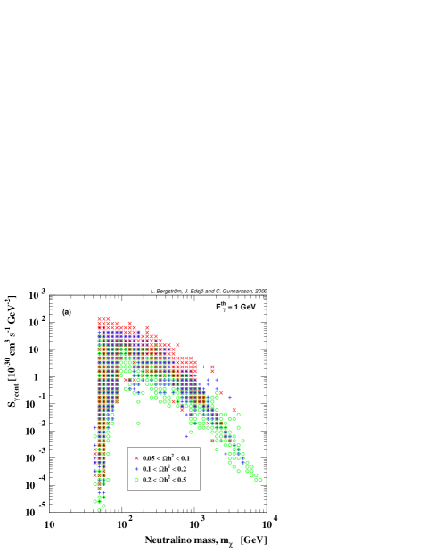
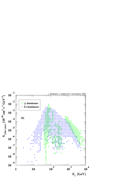
FIG. 1.: The ${\cal S}$-factor for gamma rays. In a) the continuous $\gamma$-ray flux above 1 GeV is shown versus the neutralino mass and in b) $\max({\cal S}_{\gamma\gamma},{\cal S}_{Z\gamma})$ for the monochromatic gamma ray lines is shown versus the gamma ray energy.

Gamma rays with a continuous energy spectrum mainly originate from pions produced in quark jets. We have simulated the hadronization and/or decay of the annihilation products with the Lund Monte Carlo Pythia 6.115 [23]. We have also computed the flux of monochromatic gamma lines that arise from neutralino annihilations to $\gamma\gamma$ and $Z\gamma$ at the 1-loop level [24], and which would provide an excellent signature of dark matter if detected. In Fig. 1 we plot the ${\cal S}$-factors for continuous gamma rays (above 1 GeV) and gamma ray lines respectively, where ${\cal S}$ is defined in Eq. (3). The ${\cal S}$-factors have been calculated with DarkSUSY [17]. The maximum for the continuous gamma rays is ${\cal S}_{\gamma~{}\!{\rm cont}}\sim 150\times 10^{-30}$ cm³ s^-1 GeV^-2 and occurs at $m_{\chi}=57$ GeV whereas the maximum for the monochromatic gamma ray lines is ${\cal S}_{\gamma\,{\rm line\,(max)}}\sim 0.0076\times 10^{-30}$ cm³ s^-1 GeV^-2, which occurs for annihilation into $\gamma\gamma$ at $m_{\chi}=78$ GeV. We will use these maximal values of the ${\cal S}$-factors in our estimates of the signal below to get the ‘best-case’ scenario with the highest fluxes.

C Correlation with antiproton fluxes

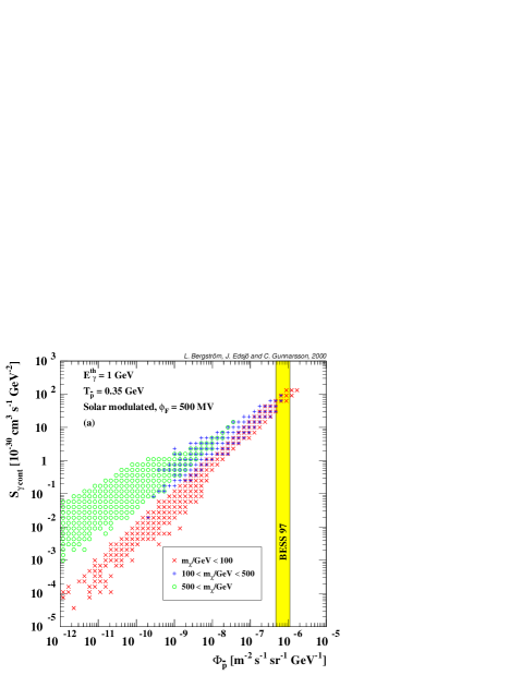
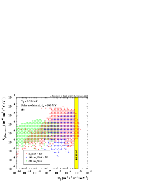
FIG. 2.: The ${\cal S}$ factors for continuous $\gamma$s and $\gamma$ lines versus the flux of antiprotons as calculated for a smooth halo.

It is well-known that whenever there is a large annihilation signal in continuous gamma-rays, there tends to be a large number of antiprotons also created [7]. This is due to the fact that both mainly emanate from quark jets formed in the annihilations. (On the other hand, antiprotons and gamma-ray lines are much more weakly correlated due to completely different production processes.) Therefore, one has to check whether the predicted gamma-ray fluxes are consistent with the present experimental bounds on antiprotons [10].

In Fig. 2 we show the ${\cal S}$ factors versus the antiproton flux as calculated in a smooth halo scenario [25] (with an isothermal sphere halo profile) and as expected, the correlation between the antiproton flux and the continuous gamma ray flux is very strong, whereas the correlation with the monochromatic gamma ray flux is weak.

We will in the following sections give predictions for the gamma-ray flux in the two structure formation scenarios (hierarchical clustering or caustics), and we also estimate how much the flux of antiprotons would increase in the two scenarios and compare with the BESS bound.

IV The Hierarchical Clustering Model

A Results from $N$-body simulations

We first consider the “standard” model of structure formation, hierarchical clustering of cold dark matter. Here we make use of the results in a recent paper by Calcáneo-Roldán and Moore [3], which we now briefly summarize. They chose from a large $N$-body simulation aimed at representing the Local Group, a simulated dark matter halo at redshift $z=0$ having a peak circular velocity of around 200 km/s and mass $10^{12}M_{\odot}$ within the virial radius of 300 kpc. They computed the local density distribution of this halo by averaging over the 64 nearest neighbours at the position of each particle in the simulation. They then estimated the flux of annihilation photons by using a discretized version of our Eq. (4), where the line of sight integral was replaced by a discrete sum over radial increments of length 1 kpc, and an angular window size $\Delta\Omega=1^{\circ}\!\times 1^{\circ}$ was used for the binning of a sky map. Since the halo used showed the characteristic triaxial, roughly prolate, shape found in $N$-body simulations (with ratio of short to long axis of 0.5 and intermediate to long axis ratio of 0.4), it is of non-negligible importance where one puts the observer (chosen to be 8.5 kpc from the center). If the long axis is in the direction of the Galactic center, the flux will obviously be higher in both the Galactic center and anticentre direction than if one of the shorter axes is in that direction. The difference can be almost an order of magnitude in directions away from the galactic center, which is an interesting point to notice, since it is independent of the existence of substructure. We will use the result where the Solar System is put on the short axis.

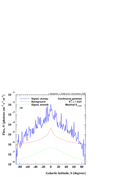
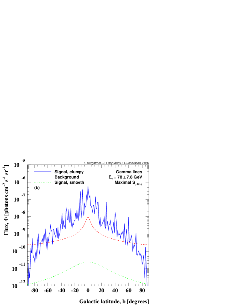
FIG. 3.: Gamma ray fluxes from substructures as seen in the $N$-body simulations in [3]. Shown is the flux averaged in strips 1^∘ high and 44^∘ wide as a function of the galactic latitude (based on Fig. 10 in [3] and on our computed ${\cal S}$-factors in Fig. 1). In a) the continuous flux above 1 GeV is shown and in b) the flux of monochromatic gamma lines is shown. In both figures, the expected diffuse background, Eq. (6) and the expected flux from a smooth isothermal sphere are shown for comparison.

In the simulations, substructure seems to be abundant on all scales, even down to velocity dispersions of a few meters per second, with a radial profile in the clumps being consistent with a very steep $\rho\propto r^{-1.5}$ behaviour. This makes the prediction of the flux very uncertain, since the line of sight integral will diverge unless a cutoff is introduced. A physically unavoidable cutoff will eventually be set by the self-annihilation rate of the dark matter particles. Unfortunately, the mass involved near the cusps of these substructure clumps is quite small and may be strongly affected by interaction with the baryonic component. This interplay of non-baryonic and baryonic matter is presently very poorly understood, to the point that even the existence of any dark matter substructure at all in cold dark matter halos is being disputed. In lack of a good description of the interplay of non-baryonic and baryonic matter, the only softening of the singularity that is included in the calculation of $J(\eta)$ is the self-interaction cut-off.

To get an estimate of the gamma ray fluxes expected in the hierarchical clustering scenario we will use Fig. 10 in Ref. [3] where the integral along the line of sight was calculated, i.e. essentially our Eq. (4) as a function of the galactic latitude, $b$ (or $\eta$ in our notation). An angular resolution of about $\Delta\Omega=1^{\circ}\!\times 1^{\circ}$ was assumed and the flux was averaged over a strip of height 1^∘ and width 44^∘. In Fig. 3, we have plotted the flux expected for the MSSM models giving the maximal continuum flux and the maximum line flux in the hierarchical clustering scenario. The diffuse background also shown can be viewed as a limit on the unexplained observed gamma ray flux. We have also plotted the flux that we would expect in a smooth halo scenario, where we have used an isothermal sphere, see Eq. (15) below, with a scale radius of $a_{\rm c}=4$ kpc, our galactocentric distance, ${\cal R}_{0}=8.5$ kpc, and the local halo density, ${\cal D}_{0}=0.3$ GeV/cm³. As can be seen, the expected flux in the hierarchical clustering scenario is very high and the maximal MSSM model chosen here would in fact already be excluded for this scenario.

It is intriguing that the angular distribution of the diffuse flux measured by EGRET is consistent with a contribution from neutralino annihilation giving a peak in the direction of the Galactic center. However, convincing evidence of a signal can only be obtained when GLAST provides also the energy spectrum in the interesting range. Of course, detection of a gamma-ray line would be a striking verification of the WIMP annihilation hypothesis.

With the fluxes given in Fig. 3, we can estimate the event rates with GLAST. Let’s focus on the peak at a galactic latitude of $b\simeq-33^{\circ}$. For continuous gammas, the flux in this peak is about $7\times 10^{-4}$ cm^-2 s^-1 sr^-1. Assuming an effective area for GLAST of $\langle A_{\rm eff}\rangle=5000$ cm² and an integration time of 1 year, this corresponds to $1.5\times 10^{6}$ events. Hence, the peak would easily be visible with GLAST, even after a reduction by a factor of ten needed for consistency with the existing background measurements. For the gamma ray lines, the fluxes are lower, and for the same peak at $b\simeq-33^{\circ}$ the flux is about $3\times 10^{-8}$ cm^-2 s^-1 sr^-1. This would correspond to about 60 events in GLAST, which since these photons are monochromatic would also be easy to see. We also see from the figure that there are other peaks with even higher fluxes that would give even higher event rates in GLAST.

With Air Cherenkov Telescopes (ACTs), sensitive to gamma radiation, these signals would also be visible, but since these need to be pointed in the a priori unknown directions of the overdensities, they can mainly be used for follow-ups if GLAST would see indications of an enhanced flux.

B Antiprotons

We now estimate the increase of the antiproton flux in the hierarchical clustering scenario compared to the smooth halo scenario. The antiproton flux depends essentially on the average of ${\cal D}^{2}$ (with ${\cal D}$ being the neutralino halo density) within the closest few kpc. We do not have access to the full $N$-body simulation results, but estimate that the increase of the integral of ${\cal D}^{2}$ locally is about the same as the increase in the gamma ray flux at high galactic latitudes. From Fig. 3, we read off that this increase is about a factor of 5–10 compared to the smooth halo scenario. Hence, we expect that the antiproton fluxes in Fig. 2 would increase by roughly this factor. For the gamma ray lines, where the correlation between the gamma ray and antiproton signal is weak, we can easily find MSSM models with high gamma ray fluxes that wouldn’t violate the BESS bound on antiprotons. For the continuous gamma ray fluxes, where the correlation is stronger, the MSSM models with the highest gamma ray fluxes, would produce an antiproton flux that is a factor of 5–10 higher than the current BESS bounds. Hence the highest flux models would seem excluded. However, the uncertainty of the predicted antiproton fluxes are about a factor of 5 and our estimate of the increased antiproton flux is uncertain by at least a factor of 2. Hence, even the highest flux models may be marginally consistent with the antiproton limits from BESS. For this reason we have chosen not to exclude them from our plot. We also note that even if we pick a model a factor of 10 lower, we would still get a continuous gamma ray flux significantly higher than the background, without having any problems with the antiproton fluxes.

C Uncertainties

We end this section with a short discussion of the uncertainties. As mentioned, the value of $J(\eta)$ depends strongly on the assumed density profile for the clumps themselves. Here, only the self-interaction cut-off has been applied, which means that these predictions should be regarded as rather optimistic. On the other hand, $J(\eta)$ is averaged over a quite large solid angle, $\Delta\Omega=1^{\circ}\!\times 1^{\circ}\simeq 0.13$ sr, whereas e.g. GLAST will have an angular resolution of about $\Delta\Omega=10^{-5}$ sr. Due to the effect of individual clumps, if one would bin the sky in $\Delta\Omega=10^{-5}$ sr bins, the fluctuations would be much larger than those seen in Fig. 3, i.e. the clumps would appear as hot spots on the sky.

V Caustic rings of Dark Matter

As another example of a model having halo structure which could give rise to potentially observable dark matter annihilation signals we now consider smooth dark matter infall onto a pre-existing galaxy. We will employ the model of Sikivie [6] for the formation of caustic rings of dark matter. We first review the parts of Sikivie’s model needed to calculate the gamma ray flux from the caustics.

A Infall model

The dark matter particles, assumed to be collisionless and having a very low intrinsic velocity dispersion, are initially put on a spherical shell. This shell will then oscillate onto and out of the galaxy producing inner and outer caustics. If the particles have initial net angular momentum, caustic rings perpendicular to the axis of rotation are formed. The caustic rings will be a persistent feature in space, as there will always be shells turning around.

By definition, the density is strongly increased where a caustic is formed. In fact, if the particles have vanishing initial velocity dispersion, $\delta_{\rm v}$, the density diverges. We will neglect the velocity dispersion when deriving the general shape and location of the caustics, but introduce $\delta_{\rm v}/c=10^{-13}$ when we consider the detailed density distribution close to the caustics. The value of the velocity dispersion is typical of what is expected for a WIMP with a mass of the order of 100 GeV. The reason is that although the relic density of a WIMP of mass $m$ is fixed by the freeze-out from chemical equilibrium at the high temperature of around $m/20$, it will stay in kinetic equilibrium through weak interactions until a temperature $T_{W}$ around 1 MeV. The primordial velocity dispersion is thus roughly $\sqrt{3T_{W}/m}\sim 5\cdot 10^{-3}\sqrt{100\ {\rm GeV}/m}$. The redshift factor since $T_{W}\sim 1$ MeV is of the order of $6\cdot 10^{11}$, giving the quoted result. It is worth to point out, however, that the effective velocity dispersion due to e.g. a clumpy infall might be much higher, significantly changing our results. We will come back to this issue in section V G.

B The density profile

We label the particles arbitrarily by a 3-parameter, $\alpha$ (which could, for instance, be the position of the particle at a given initial time). The flow of a particle is completely specified by giving for each time its spatial coordinate ${\mbox{\boldmath$\rm x$}}({\mbox{\boldmath$\alpha$}},t)$. If we have $n$ different flows at $\rm x$ and $t$, we can write the solutions of ${\mbox{\boldmath$\rm x$}}={\mbox{\boldmath$\rm x$}}({\mbox{\boldmath$\alpha$}},t)$ as ${\mbox{\boldmath$\alpha$}}_{j}({\mbox{\boldmath$\rm x$}},t)$, where $j=1,\ldots,n$. To obtain the total number of particles, $N$, we integrate the number density of particles over $\alpha$-space,

$$N=\int\frac{d^{3}N\left({\mbox{\boldmath$\alpha$}}\right)}{d\alpha_{1}d\alpha_{2}d\alpha_{3}}d^{3}\alpha.$$ (10)

Mapping onto position space gives the number density

$$d\left({\mbox{\boldmath$\rm x$}},t\right)=\sum_{j=1}^{n}\frac{d^{3}N\left({\mbox{\boldmath$\alpha$}}_{j}\left({\mbox{\boldmath$\rm x$}},t\right)\right)}{d\alpha_{1}d\alpha_{2}d\alpha_{3}}\frac{1}{\left|D\left({\mbox{\boldmath$\alpha$}},t\right)\right|_{\mbox{{${\mbox{\boldmath$\alpha$}}_{j}\left({\mbox{\boldmath$\rm x$}},t\right)$}}}}.$$ (11)

where ${\rm det}\left(\frac{\partial{\mbox{{{\mbox{\boldmath$\rm x$}}}}}}{\partial{\mbox{{{\mbox{\boldmath$\alpha$}}}}}}\right)\equiv D\left({\mbox{\boldmath$\alpha$}},t\right)$ is the Jacobian of the map ${\mbox{\boldmath$\alpha$}}\rightarrow{\mbox{\boldmath$\rm x$}}$. Wherever $D\left({\mbox{\boldmath$\alpha$}},t\right)=0$, the density will diverge, and hence caustic surfaces are associated with zeros of $D$.

FIG. 4.: Plot of points where the density exceeds 1.0 GeV/cm³. Note that for ${\cal R}_{0}=$7.9, 8.2 and 8.5 kpc, we are situated inside the tricusp.

We assume that the flow of particles is axially symmetric about the $\hat{z}$-axis (coinciding with the rotation axis of the Galaxy) and also reflection symmetric with respect to the $\hat{x}$-$\hat{y}$-plane, i.e. under reflection $z\rightarrow-z$. We also assume the dimensions of the cross-section of the caustic ring to be small compared to the ring radius. Let $R(t_{0})$ be the turnaround radius for a shell at time $t_{0}$ in the $z=0$ plane and let $a$ be the ring radius. We then parameterize the flow as ${\mbox{\boldmath$\rm x$}}(\theta_{0},\varphi_{0},t_{0};t)$, where $\rm x$ is the position vector at time $t$ of the particle that was at polar and azimuthal angles $\theta_{0}$ and $\varphi_{0}$ on the sphere of radius $R(t_{0})$ at $t=t_{0}$. Axial symmetry suggests we use cylindrical coordinates with $\varphi$-independence. Therefore we let $\rho(\alpha,t_{0};t)$ and $z(\alpha,t_{0};t)$ be the cylindrical coordinates at time $t$ of the ring of particles initially (at $t_{0}$) at $\theta_{0}=\pi/2-\alpha$. The number density can now be shown to be [6, Eq.(4.1)]

$$d\left(\rho,z,t\right)=\frac{1}{2\pi\rho}\sum_{j=1}^{n}\frac{d^{2}N\left(\alpha,t_{0}\right)}{d\alpha dt_{0}}\frac{1}{\left|D_{2}\left(\alpha,t_{0}\right)\right|}\bigg{|}_{\left(\alpha,t_{0}\right)=\left(\alpha,t_{0}\right)_{j}},$$ (12)

where

$$D_{2}\left(\alpha,t_{0}\right)=\left|\begin{array}[]{cc}\frac{\partial\rho}{\partial\alpha}&\frac{\partial\rho}{\partial t_{0}}\\ &\\ \frac{\partial z}{\partial\alpha}&\frac{\partial z}{\partial t_{0}}\end{array}\right|,$$ (13)

and $\left(\alpha,t_{0}\right)_{j}$ are the solutions of the equations $\rho=\rho\left(\alpha,t_{0};t\right)$ and $z=z\left(\alpha,t_{0};t\right)$.

In this case, the caustic condition $D_{2}=0$ becomes a fourth-degree equation in $\alpha$ having four solutions, some of which may be complex and hence unphysical. A closer inspection shows that a caustic is a border between regions with different numbers of flows. In Fig. 4 we show the cross section of the fifth caustic ring (which is the one closest to us), where regions with a density exceeding 1 GeV/cm³ have been indicated. We see that the caustic ring resembles a ‘tricusp’. Inside the tricusp, there are four flows and outside there are two. This implies that the sum in Eq. (12) should have two (four) terms if we are outside (inside) the tricusp, corresponding to the number of real roots to the caustic condition.

FIG. 5.: The maximum flux, $J(\eta_{\rm max})$ as a function of the velocity dispersion, $\delta_{\rm v}/c$. As the velocity dispersion increases from about $10^{-14}$ to $10^{-8}$, the cutoff density decreases about three orders of magnitude, from 2500 GeV/cm³ to 2.5 GeV/cm³ (with 800 GeV/cm³ at $\delta_{\rm v}/c=10^{-13}$).

The model of Sikivie has a set of caustic parameters that describe it. To find these we assume that the turnaround sphere is initially rigidly rotating and that it initially really is a sphere, not just an axially symmetric topological sphere. As mentioned, the axis of rotation for the sphere is assumed to coincide with the axis of rotation of the luminous parts of the Galaxy. We also have to make an assumption about the distribution of the smooth component of the dark matter distribution (i.e. not associated with the caustic flows). We adopt the time-independent potential

$$U(r)=-v_{\rm rot}^{2}\ln\left(\frac{R}{r}\right),$$ (14)

since this potential produces perfectly flat rotation curves with rotation velocity $v_{\rm rot}$. For comparison, we have also used the modified isothermal sphere with a density distribution

$${\cal D}_{\rm iso}(r)={\cal D}_{0}\frac{a_{\rm c}^{2}+{\cal R}_{0}^{2}}{a_{\rm c}^{2}+r^{2}},$$ (15)

where ${\cal D}_{0}$ is the local dark matter density, ${\cal R}_{0}$ is our galactocentric distance and $a_{\rm c}$ is the the scale radius, without obtaining any significant changes. To obtain the caustic parameters, we have followed the procedure in [6]. The interested reader can find the result and more details about the caustic parameters in Ref. [26]. We do not give them here since the actual values themselves are not very illuminating.

To find the density profile we first rewrite Eq. (12) into a more useful form. By reparameterizing the equation according to $t_{0}=\tau-\Delta t_{0}(\alpha)$ we have $dt_{0}=d\tau$. Due to axial symmetry, the solid angle $d\Omega=\sin\theta d\theta d\varphi$ can be rewritten as $d\Omega=2\pi\cos\alpha d\alpha$. Noting that $dN=dM/m_{\chi}$ with M being the total mass of particles with mass $m_{\chi}$ we get

$$\frac{d^{2}N}{d\alpha dt_{0}}=\frac{2\pi\cos\alpha}{m_{\chi}}\frac{d^{2}M}{d\Omega d\tau}.$$ (16)

As mentioned earlier, in this model the Solar system should be closest to caustic ring number five, and following Ref. [5], we find, for this caustic ring,

$$\frac{d^{2}M}{d\Omega d\tau}=10^{-2}\frac{V(0)v_{\rm rot}^{2}}{2\pi G},$$ (17)

where $G$ is Newton’s gravitational constant and $V(0)$ is the velocity at the point of closest approach to the Galactic center, i.e. at the caustic. This was obtained via a self-similar infall model using a scale parameter $\epsilon=0.2$ defined in Ref. [27]. However, the model dependence on $\epsilon$ is quite weak [28].

To obtain the mass density from Eq. (12) we must multiply $d(\rho,z,t)$ by $m_{\chi}$, which cancels the factor $1/m_{\chi}$ in Eq. (16). Finally, by combining Eqs. (12), (16) and (17), we can obtain the value for the mass density, ${\cal D}$, of dark matter close to the fifth caustic ring in the Milky Way.

A diverging density at the caustics results from our assumption of zero velocity dispersion, which of course is an over-simplified assumption. We thus reintroduce a non-zero velocity dispersion by estimating how much a given velocity dispersion would smear the caustic. We do that by considering a particle falling into the potential $U(r)$. If we change the initial velocity of the particle with the velocity dispersion, we obtain a difference in the location of the point of closest approach (i.e. the location of the caustic ring). We can then use this difference as an estimate of how much the caustic ring is smeared by the velocity dispersion. The simplest way to take the smearing into account is to apply a cut-off in the density whenever we are closer to the caustic than the smearing scale. For a velocity dispersion of $\delta_{v}/c=10^{-13}$, this corresponds to a cut-off in the density at ${\cal D}_{\rm cut}\simeq 800$ GeV/cm³. Since the density only diverges as $\sim 1/\sqrt{l}$ with $l$ being the distance to the caustic [4], we are not very sensitive to the actual value of the cut-off density as can be seen in Fig. 5. In our calculations we have used a cut-off density of ${\cal D}_{\rm cut}=800$ GeV/cm³.

For comparison we have also used a gaussian smearing of the density distribution with the same smearing length scale as the cut-off length scale. The two methods give practically the same result and we have used the cut-off method in our actual calculations.

TABLE II.: Summary of the peak values of $F_{\Delta\Omega}(\eta)$ for the cases considered.

$\Delta\Omega$	${\cal R}_{0}$	$\eta_{\rm max}$	$F_{\Delta\Omega}(\eta_{\rm max})$
[sr]	[kpc]	[rad]	[1021GeV2cm-5sr-1]
10-1	8.5	0.54	0.26
	8.2	0.78	0.22
	7.9	1.15	0.29
10-3	8.5	0.54	0.96
	8.2	0.79	0.91
	7.9	1.17	1.34
10-5	8.5	0.53	2.20
	8.2	0.79	4.05
	7.9	1.18	3.05

In Fig. 4, all points where ${\cal D}(\rho,z)>1.0$ GeV/cm³ are plotted. From the figure we note that for realistic values of ${\cal R}_{0}$ of about 8–8.5 kpc, we are located inside the tricusp, which is very interesting from the point of view of the possibility of detection.

Now focus on $F_{\Delta\Omega}(\eta)$. For ${\cal R}_{0}=$7.9, 8.2 and 8.5 kpc the angular range $0<\eta\lesssim\pi$ was scanned for three different typical angular acceptances, $\Delta\Omega=10^{-1},10^{-3}$ and $10^{-5}$ sr. All these scans have maxima at the angles corresponding to the cusps, since the density is strongly enhanced there. The symmetry implies a peak also at $-\eta$ if there is a peak at $\eta$. The maximum value of $F_{\Delta\Omega}(\eta)$ from all scans was found at $\eta\simeq 0.79$ rad, $\Delta\Omega=10^{-5}$ sr and ${\cal R}_{0}=8.2$ kpc. Table II gives the maximum values of $F_{\Delta\Omega}(\eta)$ for the different $\Delta\Omega$ and ${\cal R}_{0}$. The angle which gives the maximum of $F_{\Delta\Omega}(\eta)$ is denoted $\eta_{\rm max}$.

C Background to signal comparison

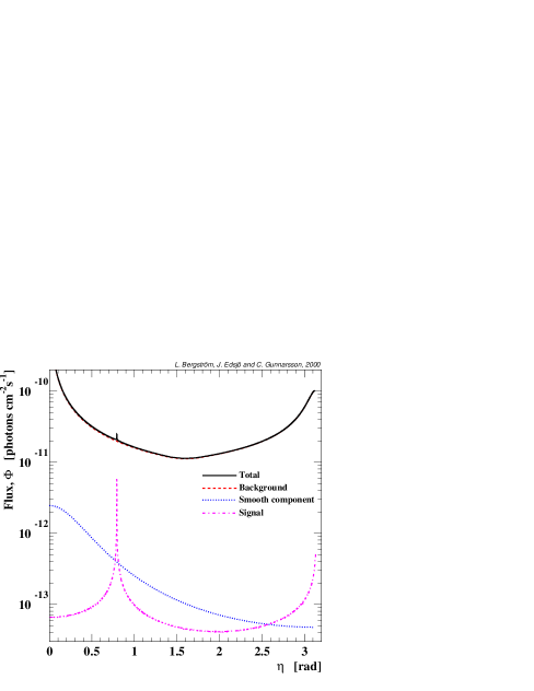
FIG. 6.: Flux of gamma rays above 1 GeV from the caustic, the smooth halo, the background and the sum of them for $\Delta\Omega=10^{-5}$ sr. A maximum flux SUSY model was used for the signal and the smooth part. For the smooth halo an isothermal sphere with the scale radius $a_{\rm c}=4$ kpc and the local density ${\cal D}_{0}=0.2$ GeV/cm³ was used. Our galactocentric distance was set to ${\cal R}_{0}=8.2$ kpc, but the results are essentially the same for other values.

To see whether the signal is potentially detectable, we have plotted the signal of continuous gamma rays from the caustic ring, the flux from annihilations in the smooth halo of Eq. (15), the background and the sum of the three in Fig. 6 for $\Delta\Omega=10^{-5}$ sr. For the smooth part we used ${\cal D}_{0}=0.2$ GeV/cm³ and $a_{\rm c}=4$ kpc. (The reason for not putting ${\cal D}_{0}=0.3$ GeV/cm³ as before is that we expect about 1/3 of the dark matter to be in the caustic flow.) Our galactocentric distance was set to ${\cal R}_{0}=8.2$ kpc, but the results are essentially the same for other values. The SUSY model used for the signal and smooth parts is one of maximum ${\cal S}$ in Fig. 1. The figure shows that the signal is quite small even for such a SUSY model and as is implied in Fig. 1, most models produce a flux several orders of magnitude smaller which would make the signal vanishingly small compared to the background. Hence, the flux shown in Fig. 6 should be regarded as a best-case scenario with the highest possible flux from the caustic rings. We thus conclude that the possibility of detection in the caustic ring model, unlike the hierarchical clustering model, is quite marginal. In Fig. 6, we plotted the continuous gamma ray flux, and for the gamma ray lines, the figure would look essentially the same, but with fluxes about a factor of $5\times 10^{-5}$ lower.

D Intensity pattern on the sky

The signal from the caustic ring is very narrowly localized in the sky angle $\eta$. To investigate how the full signal pattern would appear on the sky, we can then make the simplified assumption that the source function for the gamma-ray emission is given by a delta-function $\propto\delta^{(3)}\left({\mbox{\boldmath$\rm r$}}-{\mbox{\boldmath$\rm r$}}_{0}(\varphi)\right)$, where $\varphi$ is an azimuthal angle parameterizing the ring (see Fig. 7 for the notation).

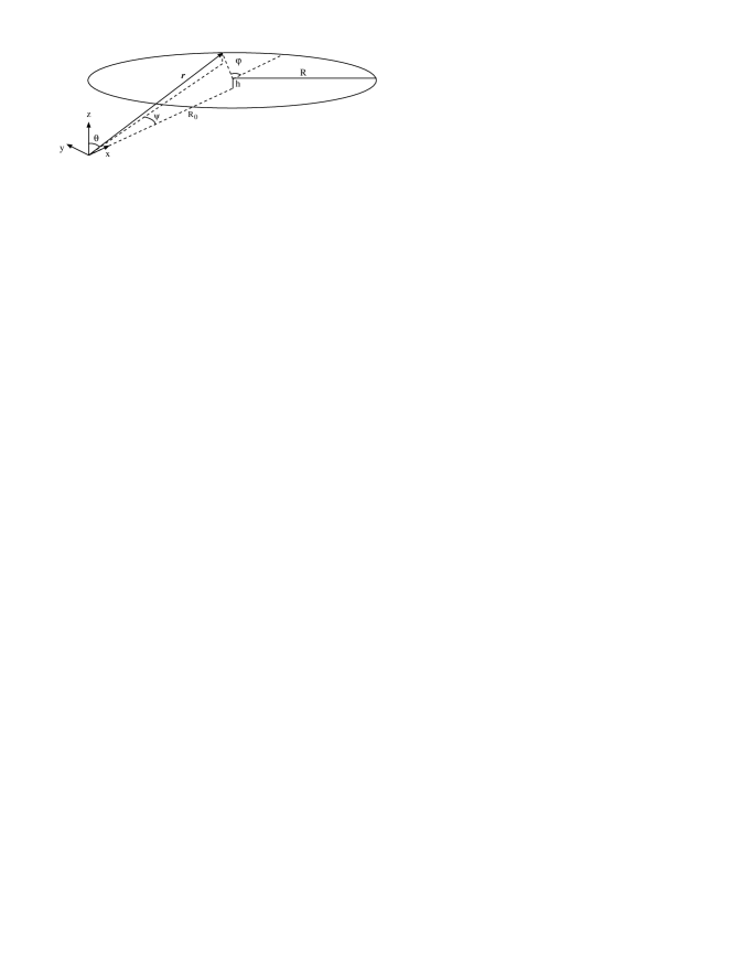
FIG. 7.: Definition of the coordinate system used.

Since each mass element of the ring locally gives rise to the same isotropic gamma-ray flux, the signal seen near the Earth’s location can be estimated analytically by geometrical considerations. Define spherical coordinates on the celestial sky $\theta$ and $\psi$ where $\theta$ is the polar angle (measured with respect to a z-axis which is tied to the Solar system and pointing perpendicularly to the plane of the Galaxy), and $\psi$ is an azimuthal angle with $\psi=0$ corresponding to the direction of the Galactic center.

We now consider one of the two closest rings corresponding to the cusps at $z\neq 0$ in Fig. 4, which are inside our position in the Galaxy, let us take the one which has $z=h>0$, and radius $R$. (Due to the $z$ symmetry, the two rings give precisely the same signal.) The location vector on the ring can be written

$${\mbox{\boldmath$\rm r$}}=(R_{0},0,h)+R(\cos\varphi,\sin\varphi,0),$$ (18)

where the point nearest to us has $\varphi=\pm\pi$, and the furthest point corresponds to $\varphi=0$. Both angles $\theta$ and $\psi$ can now be computed:

$$\cos\theta={h\over|{\mbox{\boldmath$\rm r$}}|}$$ (19)

and

$$\tan\psi={R\sin\varphi\over R_{0}+R\cos\varphi}.$$ (20)

Ring elements of constant flux $Rd\varphi{\mbox{\boldmath$\rm e$}}_{\varphi}$ are now mapped onto the sky as

$$Rd\varphi{\mbox{\boldmath$\rm e$}}_{\varphi}\rightarrow|{\mbox{\boldmath$\rm r$}}|d\theta{\mbox{\boldmath$\rm e$}}_{\theta}+|{\mbox{\boldmath$\rm r$}}|\sin\theta d\psi{\mbox{\boldmath$\rm e$}}_{\psi}=|{\mbox{\boldmath$\rm r$}}|\left({d\theta\over d\varphi}\right)d\varphi{\mbox{\boldmath$\rm e$}}_{\theta}+|{\mbox{\boldmath$\rm r$}}|\sin\theta\left({d\psi\over d\varphi}\right)d\varphi{\mbox{\boldmath$\rm e$}}_{\psi}.$$ (21)

From this we can read off the inverse of the Jacobian, which is the “magnification” $M$,

$$M={R\over|{\mbox{\boldmath$\rm r$}}|^{3}\sqrt{\sin^{2}\theta\left({d\psi\over d\varphi}\right)^{2}+\left({d\theta\over d\varphi}\right)^{2}}}.$$ (22)

where an extra factor of $|{\mbox{\boldmath$\rm r$}}|^{2}$ in the denominator accounts for the geometrical fall-off of the flux with the square of the distance. Introducing the dimensionless parameters

$$\kappa={h\over R}\qquad;\qquad\rho={|{\mbox{\boldmath$\rm r$}}|\over R}\qquad;\qquad\xi={R_{0}\over R},$$ (23)

we obtain, after some algebra,

$$\left({d\theta\over d\varphi}\right)^{2}={\kappa^{2}\over\rho^{2}-\kappa^{2}}{\xi^{2}\over\rho^{4}}\sin^{2}\varphi,$$ (24)

and

$$\left({d\psi\over d\varphi}\right)^{2}={\left(1+\xi\cos\varphi\right)^{2}\over\left(1+\xi^{2}+2\xi\cos\varphi\right)^{2}},$$ (25)

from which we can compute the flux as a function of angle on the sky by use of Eq. (22).

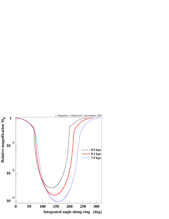
FIG. 8.: Relative magnification $M_{R}$ as a function of the integrated sky angle along the ring for three different galactocentric distances, ${\cal R}_{0}$.

We now normalize the magnification to 1 for the part of the ring that is closest to us. In Fig. 8 we show the magnification as a function of the integrated space angle along the caustic ring. We clearly see that the signal is fairly high out to about 60^∘ from the direction to the galactic center. Further away, the flux drops dramatically because of the geometric fall-off with distance.

E Detection potential

We will now investigate if the Gamma-ray Large Area Space Telescope (GLAST) [11] would be able to see even the best-case signal.

We assume the same maximal SUSY model as in Fig. 6 and use $\Delta\Omega=10^{-5}$ sr, which is close to GLAST’s expected angular resolution. We then integrate the signal over the nearest 100^∘ of the caustic ring, where the average magnification (compared to the closest part of the ring) is around 0.8 according to Fig. 8. We further assume that the average effective area will be $\langle A_{\rm eff}\rangle=5000$ cm² and that we integrate for one year. In this strip we would then expect around 400 events of continuous gamma rays above 1 GeV from the caustic ring and about 1700 events from the diffuse background as measured by EGRET. Hence, this would not be a prominent signature on the sky, especially since generic MSSM neutralinos give much lower rates. The total number of events from the gamma ray lines would be about 0.01 even in this optimistic scenario, so the prospects of detecting these are essentially zero. We end by noting that the uncertainty in the background estimate is at least a factor of two, but this hardly changes our conclusions that the gamma ray signal from the caustics is very hard to detect.

Just like in the scenario with clumps, ACTs could be used as a follow-up if GLAST would see an indication of a caustic.

F Antiprotons

To estimate the increase in the antiproton flux from the caustics, we have integrated ${\cal D}^{2}$ with a cut-off density of 800 GeV/cm³ over the region $z\in[-0.7,0.7]$ kpc and $\rho\in[7.5,9.1]$ kpc and we find that the total annihilation rate from the caustic is about 3 times higher than that from a smooth halo in the same region. Since the antiproton flux depends mainly on the total annihilation rate within the closest few kpc we don’t expect the flux of antiprotons to increase by more than a factor of 3 in the caustic scenario. We then see that for the highest values of ${\cal S}_{\gamma~{}\!{\rm cont}}$, we would get an antiproton flux that is higher than the BESS measurements by a factor of about 3. However, the antiproton flux prediction can be uncertain by as much as a factor of 5, so it is still possible that these models with high ${\cal S}_{\gamma~{}\!{\rm{cont}}}$ are consistent with the antiproton measurements and we have thus chosen not to exclude them.

G Uncertainties

We have two classes of uncertainties in this derivation of the gamma ray flux from the caustic rings. The first one comes from the fact that we don’t know the MSSM parameters and this alone gives an uncertainty of several orders of magnitude, as seen in Fig. 1. The second one are the uncertainties in the caustic model by Sikivie.

The main uncertainty is the assumption of smooth continuous infall of collisionless dark matter with a very small velocity dispersion, of the order of $\delta_{\rm{v}}/c=10^{-13}$. As $N$-body simulations seem to suggest, structure forms hierarchically and the infall to our galaxy should not be smooth, but rather clumpy. In this case, we would get an effective velocity dispersion much higher than $10^{-13}$. Some of the structures of the caustics might remain, but the significant density increase we have found here would be washed out and the signal could be reduced by orders of magnitude. On the other hand, in this case, the signal from the clumps themselves could be detectable [3] as we saw in Section IV.

The infall model itself also has some uncertainties. For instance, we have assumed that the infalling sphere is rigidly rotating, which might not be a realistic approximation. We have also assumed that the axis of rotation is the same as that of the luminous matter in our galaxy. This might depend on the details of how the bulge and disk were formed, and need not be the case.

Given these uncertainties, our strategy has been to investigate if there is a detectable signal even with the most optimistic assumptions. We have found that the detection potential is very weak although not zero under extremely optimistic assumptions.

VI Conclusions

We have supplemented the recent work by Calcáneo-Roldán and Moore based on $N$-body simulations of structure formation in cold dark matter models, by giving absolute rate predictions in the MSSM for the gamma-ray signal expected by the clumpy substructure of these simulated halos. The predicted rates are quite high, making this a promising signal to search for, both concerning continuous gamma-rays and, if supersymmetric parameters are favourable, the distinctive monoenergetic gamma-ray lines predicted if the dark matter indeed consists of WIMPs. In particular, the upcoming GLAST space-borne gamma-ray detector will be an ideal instrument searching for these intriguing patterns on the sky.

Motivated by the work done by Pierre Sikivie on caustic rings of dark matter, we have also estimated the gamma ray flux from these. However, even with very optimistic assumptions about the infall model and velocity dispersion, we can get a signal of continuous gamma rays that is only marginally detectable by GLAST. The uncertainties in the Sikivie model are large and relaxing some of the assumptions could reduce the flux further by several orders of magnitude.

However, it is worth stressing that if we relax the assumption of a smooth continuous infall, we would reduce the flux from the caustics drastically, but we would at the same time enhance the flux from the infalling clumps.

We have also investigated how much the antiproton flux is expected to increase in these two scenarios and found that for the models with the highest flux of continuous gamma rays, we would violate the BESS bound on antiprotons by a factor of about 3 in the caustic scenario and 5–10 in the hierarchical clustering scenario. Taking the uncertainties of the antiproton prediction into account, this would at best be marginally allowed by the BESS measurements. For the gamma ray lines, the correlation with the antiproton flux is weaker, and we can easily find models with high fluxes of monochromatic gamma rays that do not violate the BESS bounds.

We end by concluding that it is interesting that in two such orthogonal scenarios of galaxy formation, the outcome in both may be the existence of dark matter density enhancements which may give observable signals in upcoming gamma-ray detectors. This may indicate that the possibility of detection will exist also for refined models which describe the Milky Way dark matter distribution more realistically.