The Luminosity Function Of Field Galaxies And Its Evolution Since $z=1$

We present the B-band luminosity function and comoving space and luminosity densities for a sample of 2779 I-band selected field galaxies based on multi-color data from the CADIS survey. The sample is complete down to $I_{815}=22$ without correction and with completeness correction extends to $I_{815}=23.0$. By means of a new multi-color analysis the objects are classified according to their spectral energy distributions (SEDs) and their redshifts are determined with typical errors of $\delta z\leq 0.03$. We have split our sample into four redshift bins between $z=0.1$ and $z=1.04$ and into three SED bins E-Sa,Sa-Sc and starbursting (emission line) galaxies. The evolution of the luminosity function is clearly differential with SED. The normalization $\phi^{*}$ of luminosity function for the E-Sa galaxies decreases towards higher redshift, and we find evidence that the comoving galaxy space density decreases with redshift as well. In contrast, we find $\phi^{*}$ and the comoving space density increasing with redshift for the Sa-Sc galaxies. For the starburst galaxies we find a steepening of the luminosity function at the faint end and their comoving space density increases with redshift.

1 Introduction

The luminosity function, specifying the density of galaxies within a given comoving volume as a function of type and magnitude, is a basic ingredient in describing the galaxy population. A determination of the luminosity function at different redshifts describes in a global way the evolution of the galaxy population with cosmic look back time. Luminosity function data, combined with other data such as number counts and direct imaging data, form the observational basis for probing the statistical evolution of galaxies.

The present epoch ($z<0.2$) luminosity function is important as reference point of the evolution; there has been much controversy about its shape and normalization, but now it appears well established ( Zucca et al. (1999)) that the faint end $M_{B}\geq-16$ of the luminosity function is dominated by galaxies of later morphology, later spectral type, bluer color and stronger line emission.

To map galaxy evolution over the last half of the universe’s age, three surveys with samples of several hundred galaxies have been published in the last years: the CFRS survey (Lilly et al. (1995)) with 591 I-band selected galaxies with measured redshifts extending out to $z\approx 1$, the autofib survey (Ellis et al. (1996)) with $\geq 1700$ galaxies with redshifts $z<0.75$, and the CNOC2 survey (Lin et al. (1999)) with over 2000 R-band selected galaxies with redshifts $z\leq 0.55$. Lilly et al. (1995) found no evolution of the luminosity function for galaxies earlier than Hubble type Sb but a steepening of the faint-end luminosity function with increasing redshift for later galaxy types, i.e. the galaxy population is richer in dwarfs with increasing redshift. Such a steepening of the luminosity function has also been found by Ellis et al. (1996). In contrast, the CNOC2 survey claimed to find luminosity evolution for early type galaxy luminosity function and density evolution for the late type galaxy luminosity function, which is not in agreement with the CFRS results. Kauffmann, Charlot & White, (1996) found strong evolution in the population of the early type galaxies by re-analyzing the CFRS data, in the sense that at $z=1$ two-thirds of the nearby early type galaxy population have dropped out of the sample. However, Totani & Yoshii (1998) did not confirm this conclusion, but found that the data are consistent with passive evolution.

In this paper we present an independent determination of the luminosity function based on a new, large sample of galaxies. The CFRS, autofib and CNOC2 surveys are based on direct imaging data from which objects are separated into stars and galaxies based on morphology; then redshifts are measured for galaxies down to a certain limiting magnitude in a given band. As many faint galaxies are barely resolved, size selection effects, which can not be easily understood or modelled, enter in the determination of the luminosity function. The approach we take here is completely different. We use multi-color data and determine galaxy type and redshift from comparison to a library of color indices. This automatic process can be simulated and therefore we can reliably determine the completeness of our data. A further advantage of our 12-color data is that we do not have to apply k-corrections by fits of polynomials or the like; rather we interpolate measured data. The disadvantage of our multi-color method are redshift errors which are larger than spectroscopic ones, but we can show that they do not affect the luminosity function.

2 The Data Sample

Since CADIS will be described in detail elsewhere (Meisenheimer et al., in preparation), we only briefly summarize the most pertinent information necessary for this paper. Once finished, CADIS will cover seven $100\squareforqed\arcmin$ fields in different regions of the sky which avoid obvious foreground stars and for which the IRAS cirrus at $100\mu m$ is $\leq 2MJy/sr$. Our present analysis is based on three widely separated fields (1h, 9h and 16h field, see table 1).

Table 1: The centers of the fields

field	$\alpha_{2000}$	$\delta_{2000}$
1 h	$1^{h}47^{m}33\aas@@fstack{s}3$	$2\degr 19\arcmin 55\arcsec$
9 h	$9^{h}13^{m}46\aas@@fstack{s}5$	$46\degr 14\arcmin 20\arcsec$
16 h	$16^{h}24^{m}32\aas@@fstack{s}3$	$55\degr 44\arcmin 32\arcsec$

CADIS is a multi-color survey, using three broad band (B, R, J or K’) and up to 13 medium band ($\delta\lambda=250$ to $500\AA$) filters with central wavelengths from $3900$ to $9150\AA$. Although these filters are tailored for detection of high redshift emission line objects, the resulting multi-color photometry allows excellent classification of the objects according to their SEDs and determination of their redshifts.

Total integration times in a narrow band filter are on the order of 20 ksec on the 2.2m telescope, split into several dithered exposures; these long exposure times result in $10\sigma$ detection limits of $m\geq 23.0$ in all filters.

For object detection we use the SExtractor software package (Bertin & Arnouts (1996)) on the coadded frames for each filter. Photometry of the detected objects is done with our own software package MPIAphot. This photometry package optimizes the signal-to-noise ratio by deriving the fluxes above local background with a weighted sum and taking seeing variations into account (Röser & Meisenheimer (1991), Thommes (1996)). Since the photometry is an aperture photometry with apertures 1.3 times seeing measured on the individual frame, the magnitudes of large objects must be corrected for aperture losses. These corrections, which are dependent on the morphology of the galaxy, were derived from photometry on simulated images where the true magnitudes were known. Because the photometry is performed on individual rather than on coadded frames, realistic estimates of the photometric errors can be derived straightforwardly. Conversion of fluxes to magnitudes is based on observations of spectrophotometric standard stars and synthetic photometry, i.e. integration of the instrumental response function over the standard star spectrum. From the loci of the measured stellar main sequence we estimate that the systematic errors in absolute photometry are less than 0.03 mag in all filters. The magnitudes we use are Vega magnitudes. For each object our photometric catalogue thus contains (among other data) 10 to 13 magnitude entries, their errors and 9 to 12 color indices.

The color indices in the object catalogues are used to classify the objects into stars, galaxies and QSOs by comparing them to a color index library derived from the SEDs of stars, galaxies and QSOs. Note that we do not apply any morphological star/galaxy separation or use other criteria, the classification is entirely spectroscopic. The stellar library is taken from Pickles (1998). The QSO spectral library is based on the high signal-to-noise template spectrum Francis et al. (1991), but also includes different continuum slopes and line-widths; the final QSO spectral library contains templates with redshifts up to $z\leq 6$. The spectral library for galaxies is derived from the mean averaged spectra of Kinney et al. (1996). From these, a grid of redshifted template spectra was formed covering redshifts from $z=0$ to $z=2$ in steps of $\delta z=0.01$ and 100 different intrinsic SEDs, from old populations to starbursts. Our final library of color indices contains entries for 131 star-, 45150 QSO- and 20100 galaxy templates. Using the minimum error variance estimator, each object is assigned a type (star, QSO, galaxy), a redshift (if it is not classified as star) and an SED. The formal errors in this process depend on magnitude and type of the object and are on the order of $\delta z=0.03$ and $\delta SED=2$ (of 100). The dispersion in the estimated values does not increase with redshift for $z\leq 1.04$. Full details are given in Wolf et al. (2000).

Down to the magnitude limit $m_{I815}\geq 23.0$ in a medium band filter centered at $\lambda=815nm$, 4303 objects were detected, 835 of these were classified as stars, 69 as QSOs and 3399 as galaxies, 2779 of which are within the redshift range $z=0.1$ and $z=1.04$. For 257 objects (i.e. 6 %) neither redshift nor SED could be estimated.

In Fig. 1 we show the differential number counts of objects which are classified as galaxies and for which the classification algorithm can determine a redshift. As this figure shows, our data are effectively complete to $m_{I815}=22$; only in the faintest brightness bin we have to correct for incompleteness. The slope in the number counts from $m=18$ to $m=22$ is $0.403\pm 0.018$ and agrees well with the results of Nonino et al. (1999); fitting their data in the same magnitude range we obtain a slope of $0.39$. Fig. 2 shows the completeness of the classification as function of magnitude derived from the simulations described in section 4.

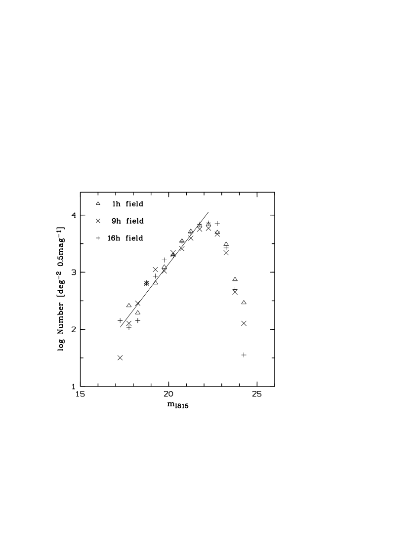
Figure 1: Differential number counts in the $I815$ filter. The data points include only those objects which were used in our analysis, i.e. objects which were classified as galaxies and for which a redshift was estimated. The straight line is the fit to these data from $m_{I815}=17.$ to $m_{I815}=22.5$

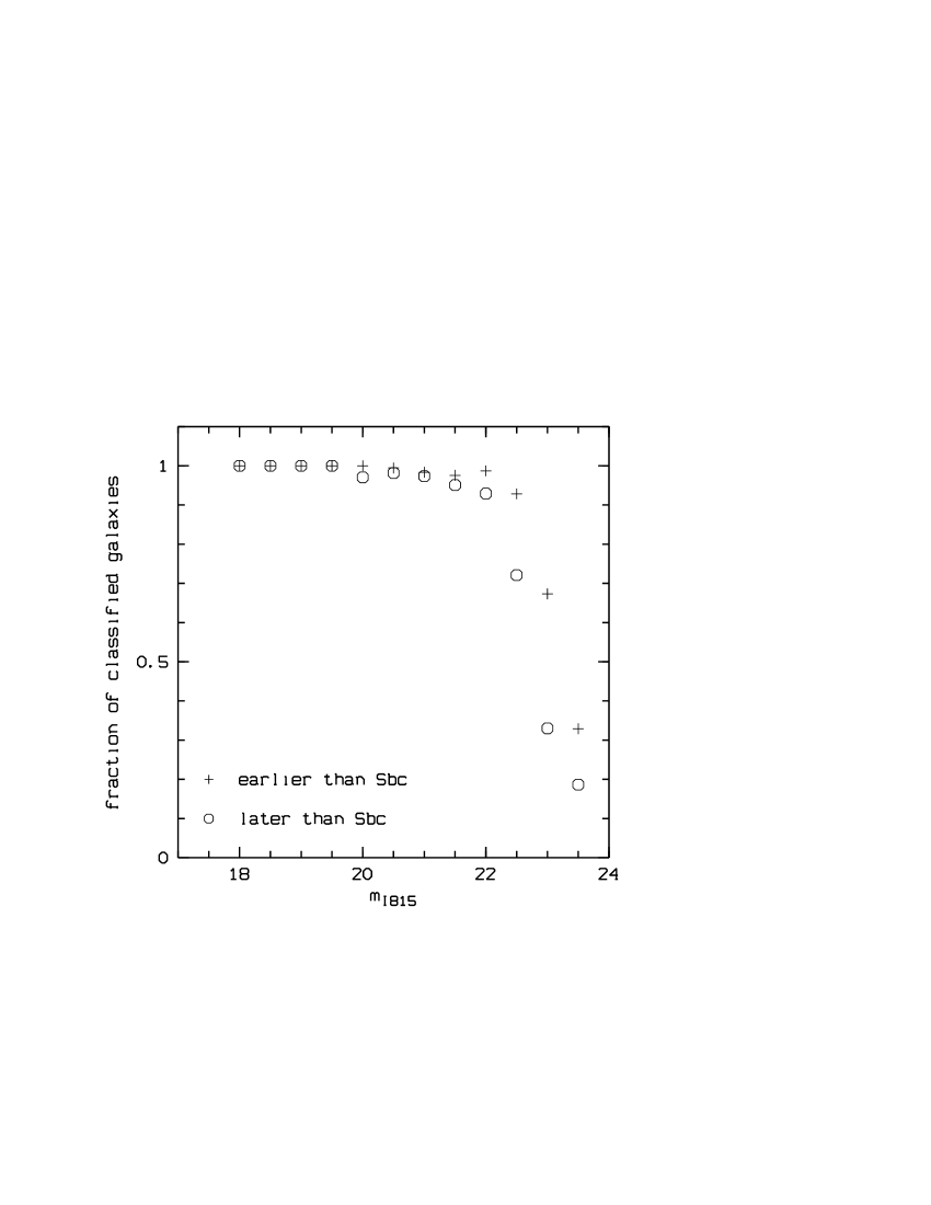
Figure 2: The completeness of the classification process derived from simulations (see sect. 4).

Lilly et al. (1995) have pointed out the advantages of selecting a sample in the I-band, which are (i) good match to B selected local samples since the B band is redshifted to I for $z\approx 0.9$ and (ii) minimization of selection effects since k-corrections are much smaller and depend less on the SED of the object in the I-band than in shorter wavelength filter bands. Put another way, surveys that select the objects at shorter wavelengths are more affected by selection effects, since at given measured B-magnitude galaxies of different morphological types will contribute to the rest frame B band luminosity function.

Since the redshifted B-band always falls between two of our filters for redshifts $z\leq 1.04$, the rest-wavelength B-magnitude is computed for all objects by interpolation between the 2 adjacent CADIS filters. We emphasize that we do not have to derive K-corrections from model spectra or polynomial extrapolations, rather we simply interpolate measured data.

Figure 3 shows our basic observational result, the location of the galaxies in the $M_{B}-z$ diagram. For consistency with earlier work the absolute B-magnitudes have been computed using $H_{0}=100\,kms^{-1}Mpc^{-1},q_{0}=0.5$. Note that at $z=1$ the inferred absolute magnitudes would be 0.6 mag brighter for an $H_{0}=100\,kms^{-1}Mpc^{-1},\Omega_{m}=0.3,\Omega_{\Lambda}=0.7$ cosmology.

The upper right portion of this M-z diagram is devoid of galaxies which reflects our magnitude limit; since this limit is set to $m=23.0$ in the $I_{815}$ filter, it appears as a sharp cutoff in the $M_{B}$ magnitudes only around $z\approx 0.8$. The region $z\leq 0.3$ is sparsely populated which is due to the relatively small field of view covered by our data; we have therefore concentrated our analysis to $z\geq 0.3$. The distribution of the galaxies in Fig. 3 shows conspicuous horizontal bands; all three fields combined show a more homogeneous distribution. Inspection of the spatial distribution of the galaxies in our fields shows that the $9h$ field contains a sheet of galaxies near $z=0.2$. Since the local bin contains only very few galaxies when the $9h$ field is taken out, we have therefore restricted our discussion to the redshift range $z=0.3-1$. A minor contribution to the inhomogeneity in redshift distribution is caused by the special choice of filters, which favors some redshifts. However, this can be corrected very well (see sect. 3.2).

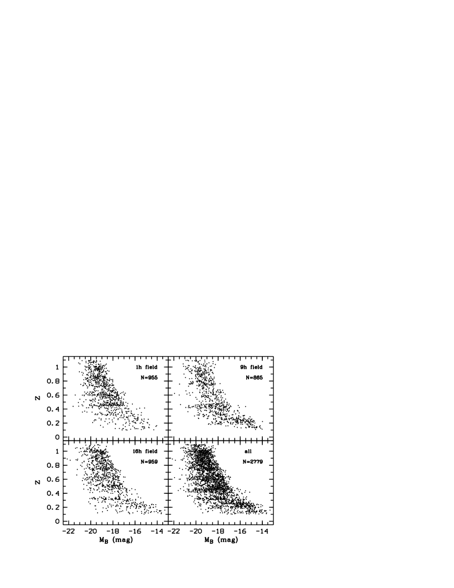
Figure 3: The $M_{B}-z$ diagrams for the galaxies in our survey for the three fields individually and combined. Absolute magnitudes calculated for a $H_{0}=100\,kms^{-1}Mpc^{-1},q_{0}=0.5$ cosmology.

3 Determination of the luminosity function

3.1 Methodology

The Schechter function is a convenient way to parametrize the luminosity function of galaxies. However, Fig. 3 illustrates that the Schechter function cannot be equally well determined at all redshifts as the segment of the luminosity function which is covered by data changes with redshift. We would expect a poor determination of $M^{*}$ for $z=0.1-0.3$ since there are few galaxies brighter than $M^{*}$ in our relatively small field of view, and a poor determination of $\alpha$ for $z\approx 1$ since there are fewer galaxies fainter than $M^{*}$ due to the magnitude limit of the survey. Since the parameters of the Schechter function are covariant, the parametric description of the luminosity function may become ill defined. Thus it is important to use both parametric and non-parametric estimations of the luminosity function.

Several estimators to derive the luminosity function from a set of M-z data have been developed in the past. We used a modified $V_{max}$ estimator as non-parametric estimate of the luminosity function and a modified maximum likelihood estimator (STY) as parametric estimate (see eg. Efstathiou, Ellis & Peterson (1988)). These modifications include an explicit completeness correction, which is given by a function $C(z_{i},SED_{i},M_{i})$ which is the probability with which a galaxy at redshift $z_{i}$ with $SED_{i}$ and absolute magnitude $M_{i}$ enters our sample. The determination of C is described in Section 3.2.

In its standard form, the $V_{max}$ estimator is computed from $\Phi(M)dM=\sum_{i}\frac{1}{V_{i}(M)}$ where $V_{i}$ is the total comoving volume in which galaxy i could lie and still be included in the sample. The volume is determined by the redshift and apparent magnitude boundaries, and the sum is taken over all galaxies in the $[M-dM/2,M+dM/2]$ interval and within a redshift interval $[z_{min},z_{max}]$. We compute the volume from

$$V_{i}={d\omega}\int_{z_{min}}^{z_{max}}C(z,SED_{i},M_{i})\frac{dV}{d\Omega dz}dz$$ (1)

where $dV/(d\Omega dz)$ is the comoving volume element per unit solid angle measured in steradians and unit redshift, and $d\omega$ is the area in steradian covered by the survey. Thus the completeness function not only corrects for detection incompleteness, but also sets the limits of the integral since $C(z_{i},SED_{i},M_{i})=0$ if an object lies outside of the survey criteria. The square roots of the variances $var(\Phi)=\sum_{i}\frac{1}{{V_{i}(M)}^{2}}$ are used as $1\sigma$ error bars on the $V_{max}$ data points.

In the STY method the probability $p_{i}$ of observing galaxy i is given by $p_{i}dM=\Phi(M_{i})dM/\int_{-\infty}^{M_{lim(z)}}\Phi(M)dM$ where $\Phi(M)$ is the luminosity function and $M_{lim(z)}$ is the absolute magnitude corresponding to the magnitude limit of the survey for the redshift of the galaxy. The completeness correction has been incorporated by replacing $\Phi(M_{i})$ with $\Phi(M_{i})C(z_{i},SED_{i},M_{i})$ so the likelihood to observe all galaxies is given by

$$L=\prod_{i=1}^{N_{obs}}\frac{\phi(M_{i})C(z_{i},SED_{i},M_{i})}{\int_{-\infty}^{+\infty}\Phi(M)C(z_{i},SED_{i},M)dM}$$ (2)

where $N_{obs}$ is the total number of galaxies in the (sub)sample. Here again the completeness function C also sets the limits of the integral. The best parameters $\alpha$ and $M^{*}$ are found by maximizing $\ln L$. Errors in these paramaters are derived from the likelihood contours at $\ln L-\frac{1}{2}\Delta\chi^{2}$ where $\Delta\chi^{2}$ is the change in $\chi^{2}$ corresponding to the desired confidence level for 2 degrees of freedom. It should be noted that these errors underestimate the true ones, because they do not account for the cosmic inhomogeneities apparent from Fig. 3. Since the normalization factor $\Phi^{*}$ cancels out in equation 2 we have determined it from $\Phi^{*}=N_{obs}/N_{pred}$ where

$$N_{pred}={d\omega}\int_{z_{min}}^{z_{max}}\int_{-\infty}^{+\infty}\frac{dV}{d\Omega dz}\Phi(M)C(z,M)dzdM$$ (3)

is the predicted number of galaxies using the derived parameters $\alpha$ and $M^{*}$ in the luminosity function $\Phi(M)$, and $C(z,M)$ is the mean of C over all SEDs. The error of $\Phi^{*}$ was determined through bootstrapping.

3.2 Completeness Correction

The completeness function C was determined as follows. For a given set of colors and their errors, the color classification algorithm (Wolf et al. 2000) estimates redshift and SED for each object. After this classifying process an object drawn from a given point ($SED_{i},z_{i},M_{B_{i}}$) in the 3 dimensional parameter space will appear at $(SED_{i}^{\prime},z_{i}^{\prime},M^{\prime}_{B_{i}})$. Even for random measurement errors the expectation value of this latter point in the parameter space is not necessarily identical to the original one, so the observed parameter space may have systematic over- or underdensities introduced by the classification process. Furthermore, the object may not be classified at all which indeed sets the completeness limit to our data. However, both completeness limit and possible classification systematics can be effectively calculated and corrected by Monte Carlo simulations of the observations.

From the galaxy template library we have constructed a grid of 625191 input “objects” brighter than $m_{I815}=23.5$ in the 3 dimensional parameter space $SED-z-M_{B}$ where $0<SED<100$, $0<z<1.1$ , $-12<M_{B}<-24$. Apparent magnitudes were calculated for each object corresponding to its redshift and Gaussian noise was added, matching the real measurement errors. Then this catalogue of simulated objects was passed through the classifying process and a new $M_{B_{i}^{\prime}}$ using the redshift $z_{i}^{\prime}$ estimated by the classifying routine was calculated.

Dividing the $SED-z-M_{B}$ parameter space into cells, the completeness function $C(z,SED,M_{B})$ in each cell is obviously given by the ratio objects classified to be in that cell ${N_{SED_{i}^{\prime},z_{i}^{\prime},M_{B_{i}^{\prime}}}}$ to objects initially in it:

$$C(z_{i},SED_{i},M_{i})=\frac{N_{SED_{i}^{\prime},z_{i}^{\prime},M_{B_{i}^{\prime}}}}{N_{SED_{i},z_{i},M_{B_{i}}}}.$$ (4)

The parameter space was devided into 25500 cells.

The determination of C was done separately for the two cosmologies; in Fig. 4 we show 2 D averages for $SED=0-50$ and $SED=50-100$ for the $\Omega_{m}=1,\Omega_{\Lambda}=0$ cosmology. It is obvious that the classification process favors some regions of the redshift space and discriminates against others; this is probably caused by the special choice of the wavelengths of the filters we are using. However, since our definition of C allows $C>1$, this effect is fully taken into account in the corrections for $V_{max}$ (Equation 1) and in the maximum likelihood estimation (Equation 2).

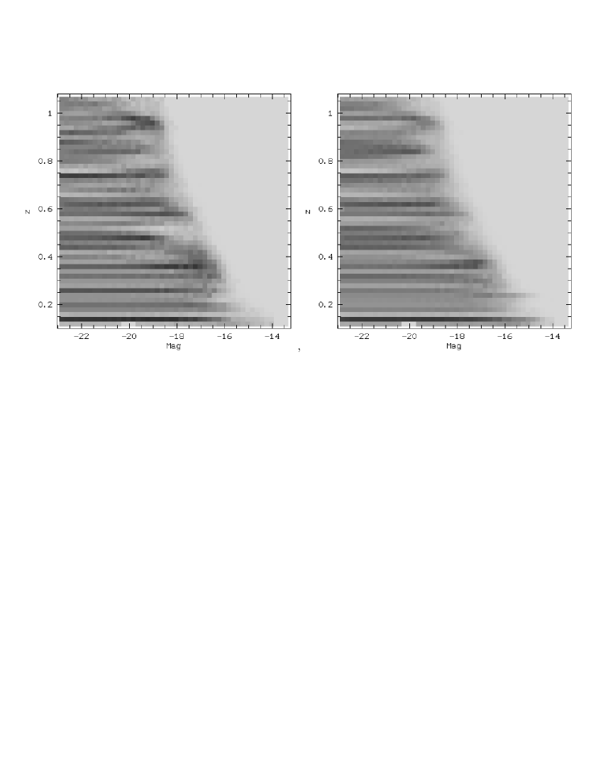
Figure 4: The completeness correction function C for galaxies earlier than Sbc(left) and galaxies later than Sbc (right). The grey scale coding is linear from C=0 (white) to C=2 (black).

4 Monte Carlo Simulations

The effect of photometric errors on the luminosity functions was studied by Monte Carlo simulations. An advantage of our purely photometric classification is the possibility to simulate the complete process, including the redshift assignments to the objects. Though the errors of our photometric redshifts are on the order of $\delta z=0.04$ and thus larger than typical spectroscopic redshift errors, one would expect that their effect is small since they lead to errors in absolute magnitude $\delta M=0.08$ which are much less than the 1-mag bins we are using for calculating the luminosity function. Nevertheless, we have examined the effect of redshift errors by numerical simulations.

Simulated galaxies were distributed in the M-z plane with a redshift distribution that corresponds to a constant comoving volume density and with absolute magnitudes drawn from a Schechter function with $M^{*}=-19.5,\alpha=-1.0$ for all types of galaxies. The SEDs were randomly distributed in the interval $[0,100]$. Apparent magnitudes were calculated using the $\Omega_{m}=1,\Omega_{\Lambda}=0$ cosmology and noise added to the color indices according to the actual measurement process for all artificial galaxies. These objects were then run through the classifying process. For $m_{I815}>22.0$ $94\%$ of the input galaxies were classified as such, and $86\%$ of the galaxies have redshift errors $\leq\pm 0.05$. In the center of our last magnitude bin $m_{I815}=22.5$, the corresponding numbers are $82\%$ and $72\%$, respectively. The classification completeness is shown in Fig. 2. In this manner we have formed 5 samples of galaxies with the number of galaxies in each sample roughly as in our data. For these samples we have then determined the luminosity function as for the real galaxies.

The agreement between the input and the recovered Schechter parameters is excellent in the redshift range $z=0.3-0.9$ where we find displacements in characteristic magnitude $|\delta M^{*}|\leq 0.05$ and slope $|\delta\alpha|\leq 0.02$. As expected, the parameters are less well recovered for $z=0.1-0.3$ and $z\geq 0.9$: we obtained $M^{*}=-19.2$, $\alpha=-0.82$ for $z=0.1-0.3$ and $M^{*}=-19.84$, $\alpha=-1.31$ for $z>0.9$. The numbers given here apply to both early and late type galaxies; we found no significant dependence on SED type.

These simulations thus show that we can recover the luminosity function parameters very well for $z=0.3-0.9$. The displacements of the recovered parameters are smaller than their errors in the actual data. For redshifts outside the $z=0.3-0.9$ range the description of the luminosity function by the parameters of the Schechter function becomes poor. However, even if the parameters are well determined, it may be dangerous to draw conclusions on the luminosity function from the parameters alone because they are coupled: for example, a decrease in $M^{*}$ is compensated by an increase in $\alpha$ - the error ellipses in Figs. 6 to 11 demonstrate this very clearly - and consequently by a decrease in $\phi^{*}$. Therefore the non-parametric form of the luminosity function is indispensable.

5 Results

5.1 The local luminosity function

Because of the sheet of galaxies contained in the $9h$ field and the resulting problems (see sect. 2), our results for the local redshift bin are preliminary until CADIS is completed. Nevertheless we show the luminosity function for all galaxies with $z=0.1-0.3$ in Fig. 5. The derived Schechter function is described by $\phi^{*}=0.0156\pm 0.004,M^{*}=-19.2\pm 0.27,\alpha=-1.30\pm 0.069$. This is agrees within the errors with an eyefitted mean of recent determinations by Zucca et al. (1999), Loveday (1997), Marzke & da Costa (1997), Marzke, Huchra & Geller (1994) and Folkes et al. (1999) which is described by $\phi^{*}=0.017,M^{*}=-19.6,\alpha=-1.15$.

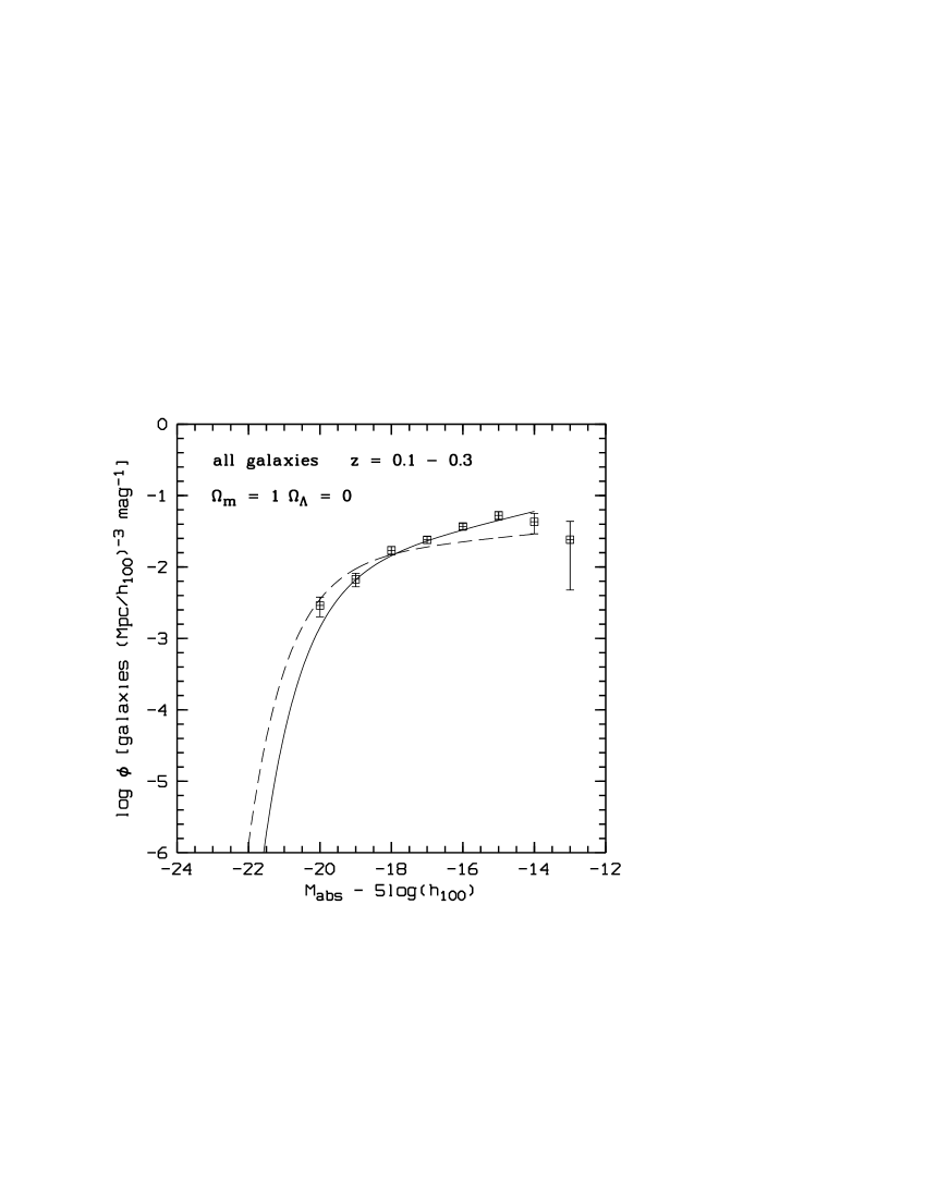
Figure 5: The luminosity function of the 439 galaxies in our sample with $z=0.1-0.3$. The data points were derived from the $V_{max}$ method, the solid line is the Schechter function derived from the STY method, the dashed line is the mean of recent determinations of the local luminosity function.

5.2 Evolution of the luminosity function

It has been well established that the local luminosity function is different for early and late type galaxies in the sense that the slope $\alpha\approx-0.8$ for early type galaxies which are dominated by old populations and $\alpha\approx-1.8$ for late type galaxies which are dominated by starforming populations (Marzke et al. (1994)), i.e. the starforming galaxy population is richer in dwarfs. Furthermore, other redshift surveys have found a dependence of the evolution of the luminosity function on galaxy type. We have therefore divided our sample into three SED bins, E-Sa galaxies with $SED\leq 30$, Sa-Sc galaxies with $30<SED<75$ and starforming galaxies with $SED>75$ (Wolf et al. (2000), Kinney et al. (1996)). We have further divided our sample into three redshift bins $z=0.3-0.5$, $z=0.5-0.75$ and $z=0.75-1.04$.

To facilitate comparison with other work we have derived the luminosity function for an $H_{0}=100\,kms^{-1}Mpc^{-1},q_{0}=0.5$ cosmology. We also give the results for a cosmology with $\Omega_{m}=0.3,\Omega_{\Lambda}=0.7$; in order to show the effects of cosmic acceleration in a transparent manner, we have again used $H_{0}=100\,kms^{-1}Mpc^{-1}$. For $H_{0}=62\,kms^{-1}Mpc^{-1}$ the conversion relations are $M_{62}=M_{100}-1.02$ and $\phi^{*}_{62}=\phi^{*}_{100}\times 4.2$. Since the effects of the cosmology on the luminosity functions and comoving space densities are mild, we concentrate the discussions on the $q_{0}=0.5$ cosmology. The results are summarized in Figs. 6 to 11 and table 2.

As Figs. 6 - 9 show, the luminosity functions of early type galaxies E-Sa have indistinguishable $M^{*}$ and $\alpha$ whereas $\phi^{*}$ decreases with redshift. For the Sa-Sc galaxies $M^{*}$ and $\alpha$ are constant, too, but $\phi^{*}$ is increasing with redshift. Note that the luminosity function of the starbursting galaxies with $z=0.75-1.04$ depends sensitively on a few bright galaxies in the $M=-22$ bin. Nevertheless, a steepening of the luminosity function with redshift is clearly evident.

,               ,

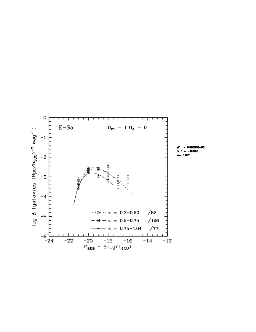
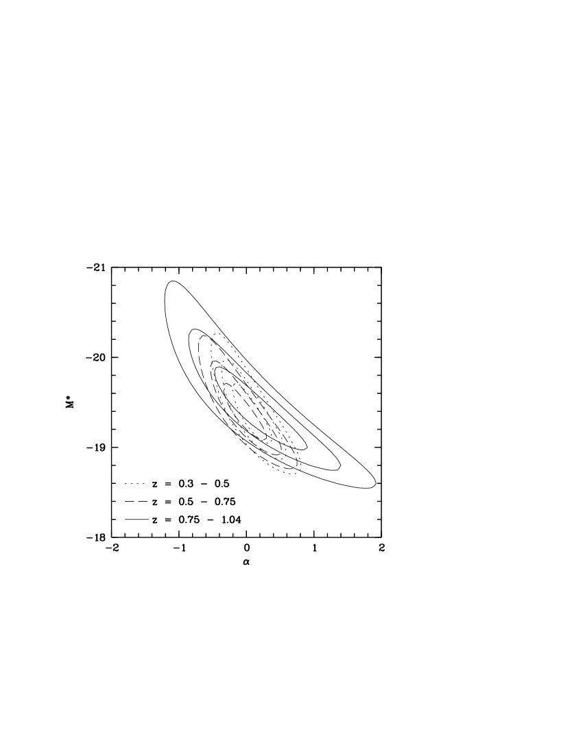
Figure 6: Left panel: The luminosity function of early type galaxies E-Sa for a $H_{0}=100\,kms^{-1}Mpc^{-1},q_{0}=0.5$ cosmology. $V_{max}$ data points with $1\sigma$ error bars and Schechter functions derived from the STY method are shown. The numbers are the numbers of galaxies in the corresponding redshift bin. Right panel: $1\sigma$ and $2\sigma$ error contours.

,               ,

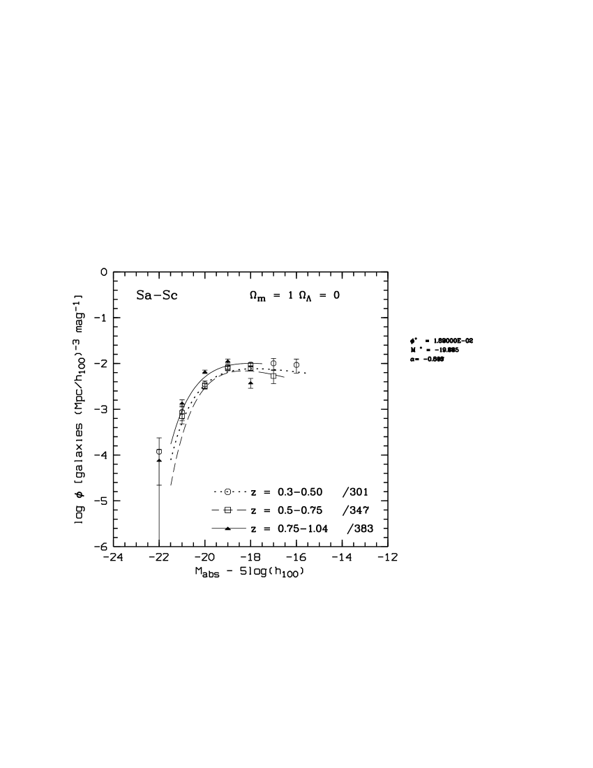
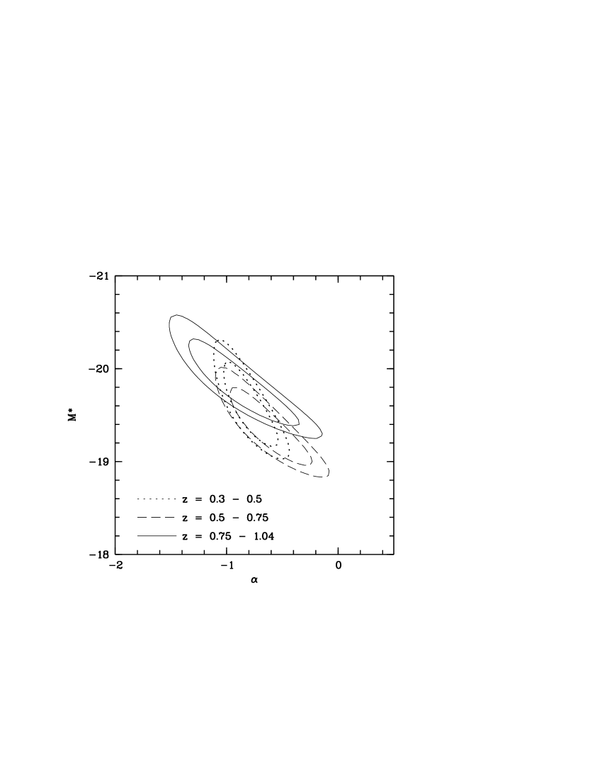
Figure 7: Same as Fig. 6 but for galaxies of types Sa-Sc.

,               ,

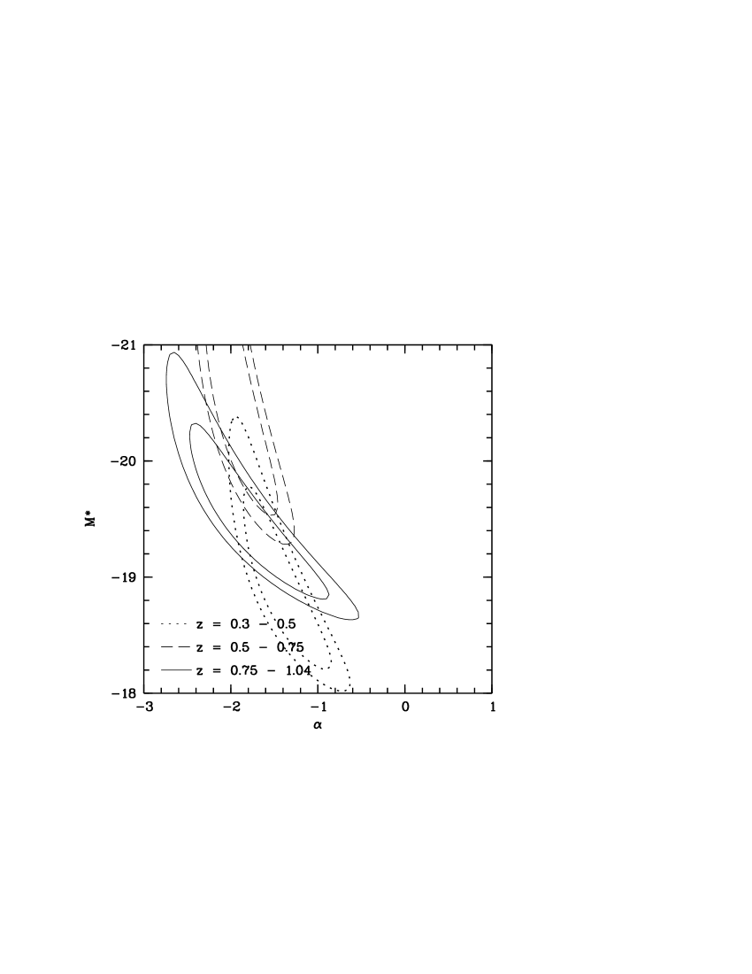
Figure 8: Same as Fig. 6 but for starbursting galaxies

,               ,

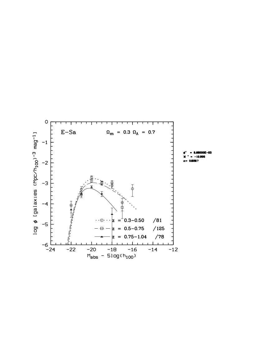
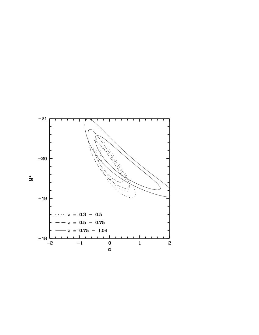
Figure 9: Same as Fig. 6 but for a $H_{0}=100\,kms^{-1}Mpc^{-1},\Omega_{m}=0.3,\Omega_{\Lambda}=0.7$ cosmology.

,               ,

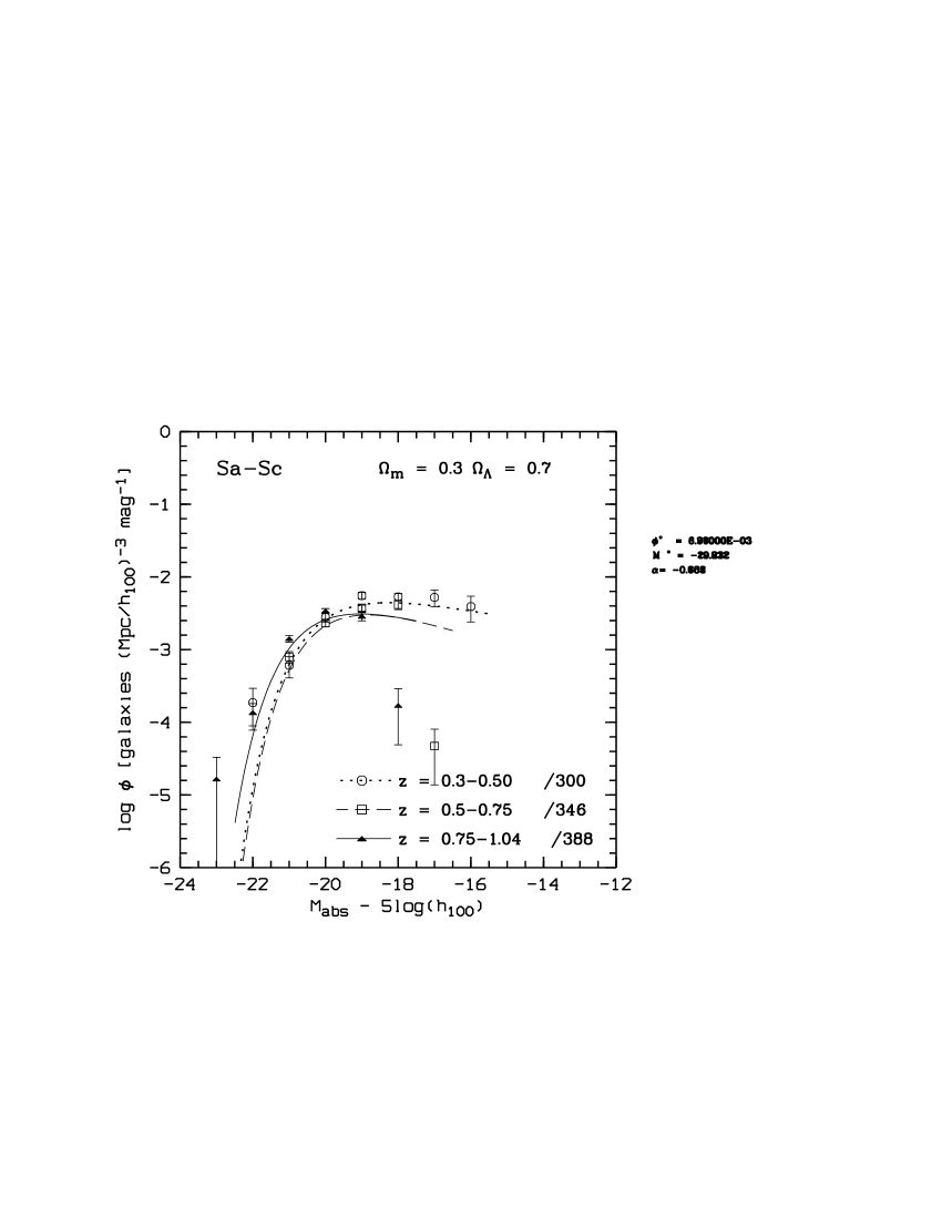
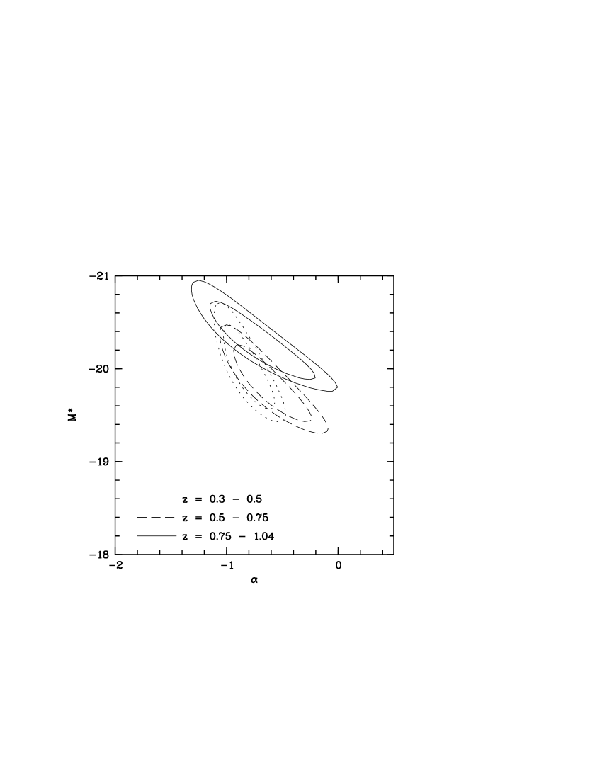
Figure 10: Same as Fig. 9 but for galaxies of types Sa-Sc

,               ,

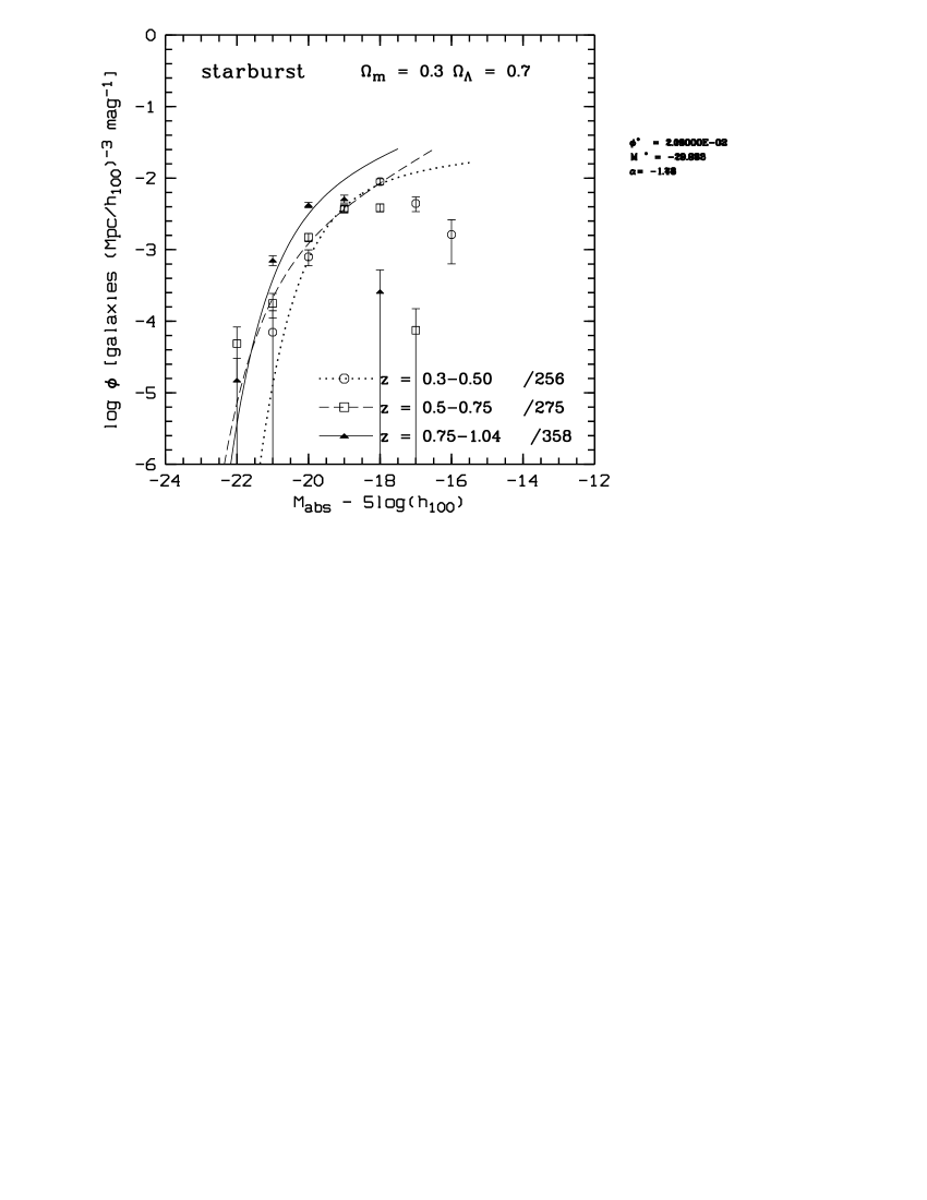
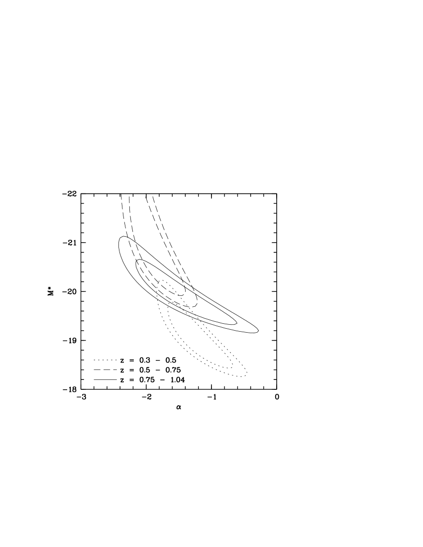
Figure 11: Same as Fig. 9 but for starbursting galaxies

To avoid the covariances in the parametric form of the luminosity function, we have also analysed the comoving galaxy space density and luminosity density as function of redshift in a way which is completely independent of the luminosity function. Since our data are virtually complete to $M_{B}=-18.5$ (see Fig.3) for all redshifts, we have integrated the numbers and luminosities, respectively, for galaxies brighter than this limit without completeness correction. The resulting comoving densities are shown as function of redshift in the Figs. 12 and 13 and the parameters of linear fits to these data are given in table 3.

For the $q_{0}=0.5$ cosmology, we find a decreasing comoving space density of the early type galaxies. The space density increases with redshift for the Sa-Sc galaxies as well for the starburst galaxies. The behaviour of the B-band comoving luminosity density is similar. For an $\Omega_{m}=0.3,\Omega_{\Lambda}=0.3$ cosmology, the trends in the data are similar but with reduced gradients.

As customary, we have calculated the errors based on Poisson statistics. This is correct as long as the total volume sampled by the survey is considered, where large-scale structure averages out. The scatter in fig.1 agrees with Poisson statistic. However, if the survey is devided into smaller subvolumes, cosmic variance due to clustering of galaxies increases the actual uncertainties. Fig.14 shows the field to field variations using the same SED and redshift bins as applied in the determination of the luminosity function. The scatter in figs.12 and 13 is higher than Poisson by factors of a few. If this is taken into account, the decrease in comoving galaxy space density for the E-Sa galaxies with increasing redshift is statistically not significant, the increasing space density of the Sa-starburst galaxies towards earlier epochs, however, still is significant. We emphasize that this problem of clustering exists with all previous surveys; quite contrary, our survey is much larger and will be still larger once all targeted fields are available.

,         ,

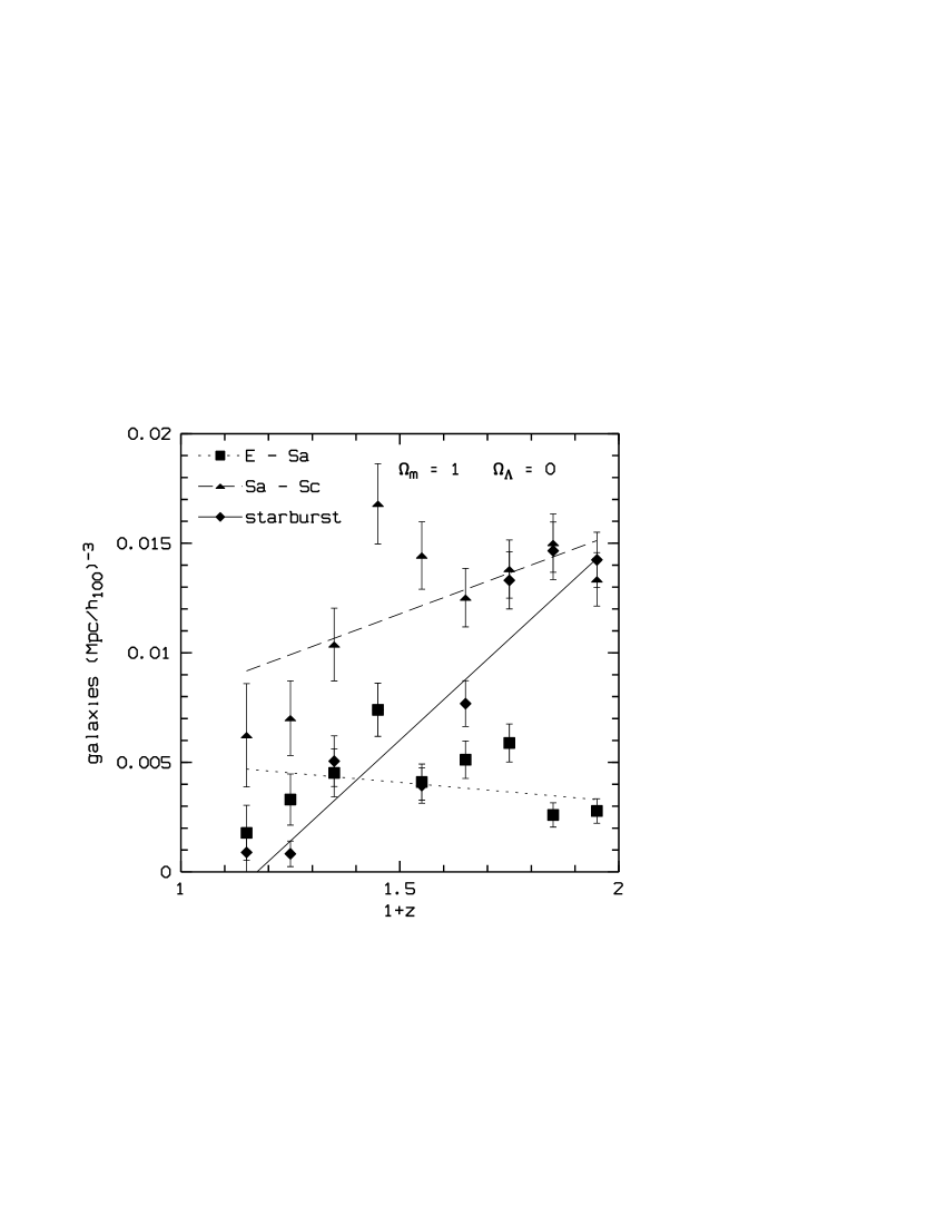
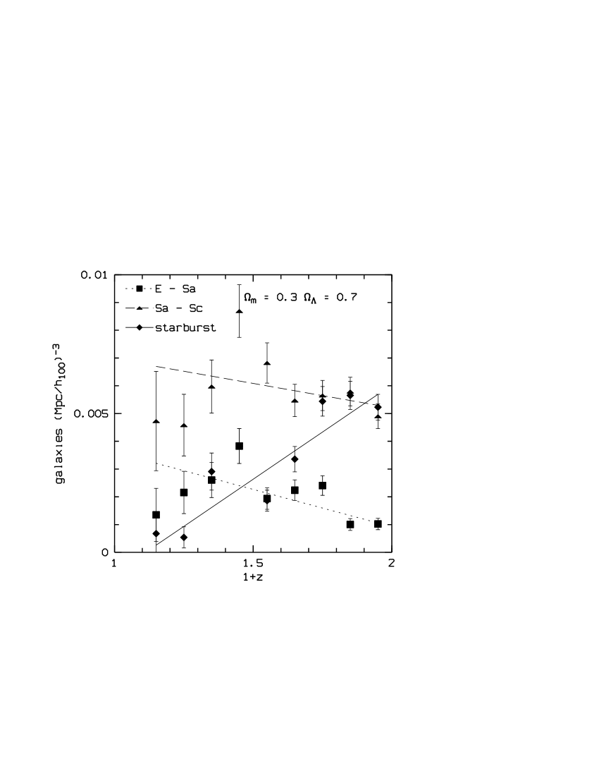
Figure 12: The evolution of the comoving number density of galaxies $M_{B}<-18.5$ for the two cosmologies. Note the different scaling of the ordinates.

,         ,

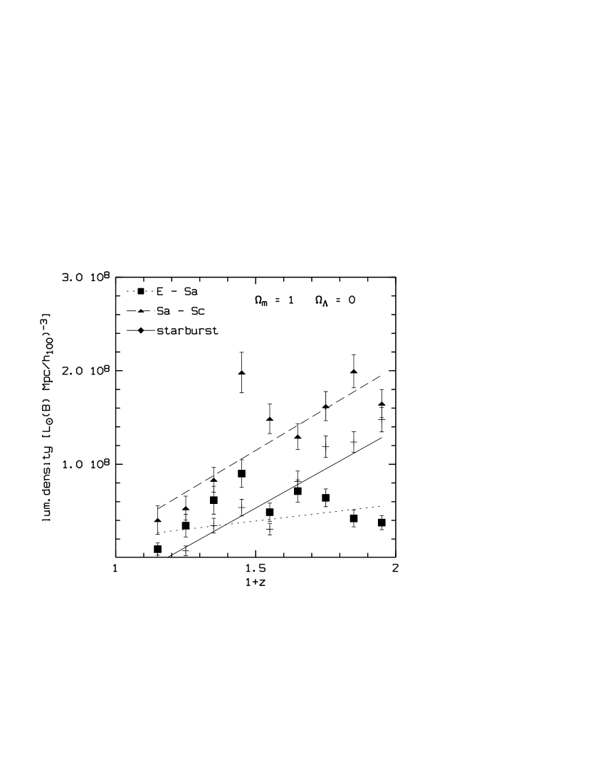
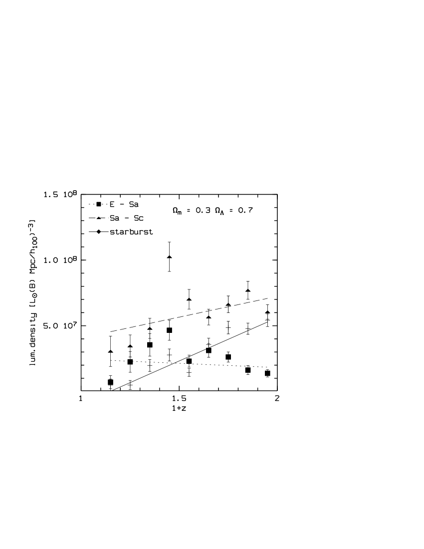
Figure 13: The evolution of the comoving B-band luminosity density of galaxies $M_{B}<-18.5$ for the two cosmologies. Note the different scaling of the ordinates.

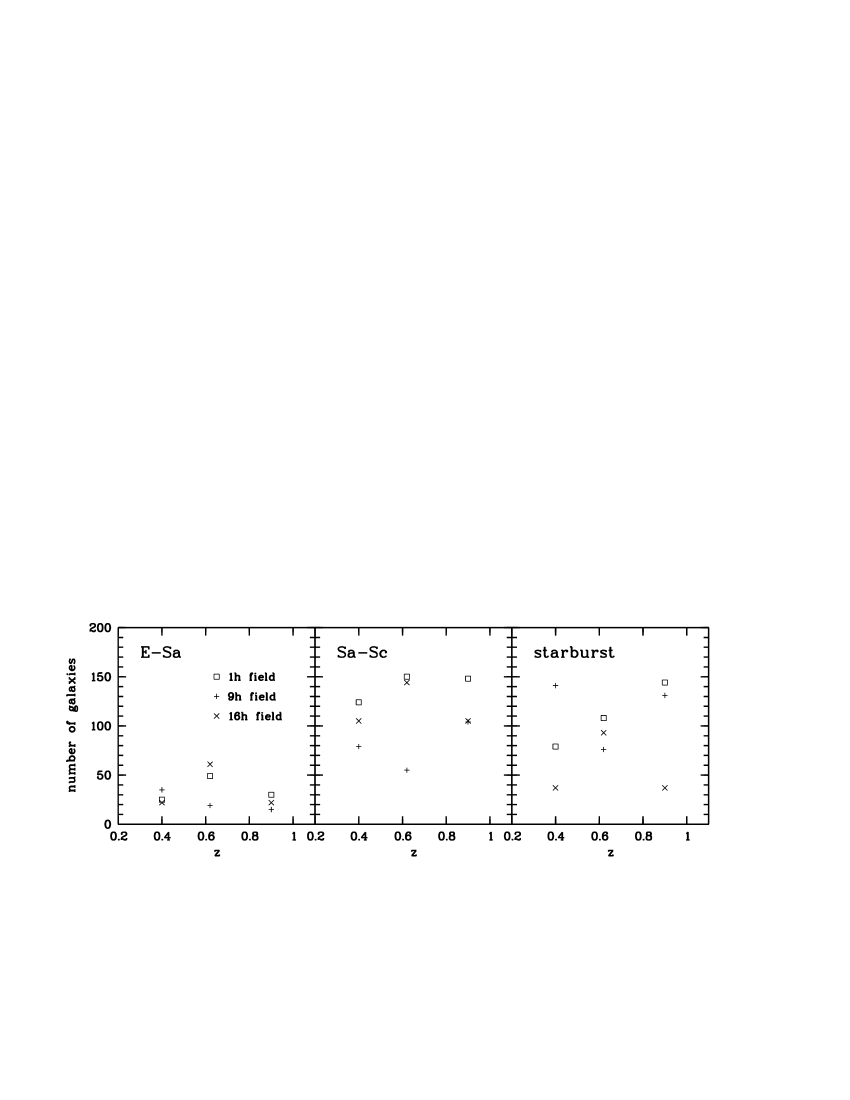
Figure 14: The field to field variations of the number of galaxies used in the determination of the luminosity functions.

Table 2: Parameters of Schechter function fits to the data.

		$\Omega_{m}=1$
sample	z range	$\phi*$	$M^{*}$	$\alpha$
E-Sa	0.3-0.5	$0.901\,10^{-2}\pm 0.559\,10^{-3}$	$-19.287\pm 0.219$	$0.187\pm 0.224$
E-Sa	0.5-0.75	$0.746\,10^{-2}\pm 0.487\,10^{-3}$	$-19.355\pm 0.180$	$-0.25\,10^{-2}\pm 0.194$
E-Sa	0.75-1.04	$0.455\,10^{-2}\pm 0.562\,10^{-3}$	$-19.360\pm 0.337$	$0.282\pm 0.52$
Sa-Sc	0.3-0.5	$0.137\,10^{-1}\pm 0.355\,10^{-2}$	$-19.660\pm 0.295$	$-0.815\pm 0.129$
Sa-Sc	0.5-0.75	$0.159\,10^{-1}\pm 0.216\,10^{-2}$	$-19.335\pm 0.158$	$-0.615\pm 0.128$
Sa-Sc	0.75-1.04	$0.182\,10^{-1}\pm 0.462\,10^{-2}$	$-19.770\pm 0.268$	$-0.807\pm 0.295$
starburst	0.3-0.5	$0.177\,10^{-1}\pm 0.715\,10^{-2}$	$-18.690\pm 0.292$	$-1.282\pm 0.209$
starburst	0.5-0.75	$0.281\,10^{-2}\pm 0.273\,10^{-2}$	$-20.27\pm 0.400$	$-1.857\pm 0.168$
starburst	0.75-1.04	$0.265\,10^{-1}\pm 0.102\,10^{-1}$	$-19.441\pm 0.227$	$-1.727\pm 0.271$
		$\Omega_{m}=0.3,\Omega_{\Lambda}=0.7$
sample	z range	$\phi*$	$M^{*}$	$\alpha$
E-Sa	0.3-0.5	$0.488\,10^{-2}\pm 0.275\,10^{-3}$	$-19.602\pm 0.178$	$0.207\pm 0.178$
E-Sa	0.5-0.75	$0.315\,10^{-1}\pm 0.332\,10^{-3}$	$-19.871\pm 0.276$	$-0.475\,10^{-1}\pm 0.221$
E-Sa	0.75-1.04	$0.144\,10^{-2}\pm 0.301\,10^{-3}$	$-19.705\pm 0.316$	$0.625\pm 0.587$
Sa-Sc	0.3-0.5	$0.831\,10^{-2}\pm 0.139\,10^{-2}$	$-19.911\pm 0.193$	$-0.782\pm 0.892\,10^{-1}$
Sa-Sc	0.5-0.75	$0.697\,10^{-2}\pm 0.971\,10^{-3}$	$-19.832\pm 0.159$	$-0.605\pm 0.159$
Sa-Sc	0.75-1.04	$0.676\,10^{-2}\pm 0.115\,10^{-2}$	$-20.232\pm 0.194$	$-0.667\pm 0.219$
starburst	0.3-0.5	$0.119\,10^{-1}\pm 0.360\,10^{-2}$	$-18.970\pm 0.233$	$-1.141\pm 0.184$
starburst	0.5-0.75	$0.211\,10^{-2}\pm 0.162\,10^{-2}$	$-20.365\pm 0.299$	$-1.730\pm 0.147$
starburst	0.75-1.04	$0.108\,10^{-1}\pm 0.329\,10^{-2}$	$-19.892\pm 0.203$	$-1.480\pm 0.276$

Table 3: Parameters of linear fits of the form $a+b(1+z)$ to the comoving galaxy density and B-band luminosity density. Absolute terms $a$ are given in the 2., slopes $b$ in the 3. column

	$\Omega_{m}=1,\Omega_{\Lambda}=0,\Omega_{\Lambda}=0$
	a	b
number density E-Sa	$0.669\,10^{-2}\pm 0.192\,10^{-2}$	$-0.174\,10^{-2}\pm 0.111\,10^{-2}$
number density Sa-Sc	$0.681\,10^{-3}\pm 0.339\,10^{-2}$	$0.744\,10^{-2}\pm 0.205\,10^{-2}$
number density starburst	$-0.216\,10^{-1}\pm 0.191\,10^{-2}$	$0.184\,10^{-1}\pm 0.129\,10^{-2}$
luminosity density E-Sa	$-0.138\,10^{8}\pm 0.163\,10^{8}$	$0.354\,10^{8}\pm 0.103\,10^{8}$
luminosity density Sa-Sc	$-0.153\,10^{9}\pm 0.300\,10^{8}$	$0.179\,10^{9}\pm 0.193\,10^{8}$
luminosity density starburst	$-0.198\,10^{9}\pm 0.163\,10^{8}$	$0.167\,10^{9}\pm 0.113\,10^{8}$
	$\Omega_{m}=0.3,\Omega_{\Lambda}=0.7$
	a	b
number density E-Sa	$0.630\,10^{-2}\pm 0.104\,10^{-2}$	$-0.289\,10^{-2}\pm 0.583\,10^{-3}$
number density Sa-Sc	$0.871\,10^{-2}\pm 0.181\,10^{-2}$	$-0.175\,10^{-2}\pm 0.105\,10^{-2}$
number density starburst	$0.630\,10^{-2}\pm 0.104\,10^{-2}$	$-0.269\,10^{-2}\pm 0.583\,10^{-3}$
luminosity density E-Sa	$0.309\,10^{8}\pm 0.100\,10^{8}$	$-0.640\,10^{7}\pm 0.582\,10^{7}$
luminosity density Sa-Sc	$0.899\,10^{7}\pm 0.164\,10^{7}$	$0.317\,10^{8}\pm 0.989\,10^{7}$
luminosity density starburst	$-0.756\,10^{8}\pm 0.878\,10^{7}$	$0.659\,10^{8}\pm 0.567\,10^{7}$

5.3 Comparison with other work

Since the luminosity function depends strongly on galaxy type, a comparison between results obtained from samples selected with different selection criteria is difficult if not impossible. In a similar way, division into differing subsamples causes differences in the luminosity function. Furthermore, different ways to estimate K-corrections can introduce redshift dependent effects. Photometric errors should be negligible if CCD data are used.

The CFRS ( Lilly et al. (1995)) is the survey which compares most directly to CADIS: their objects are also I-band selected across an identical redshift range. Since the number of galaxies included in our analysis is nearly four times as large, we have better statistics. Furthermore, our survey goes deeper by $0.5mag$ and so the range in luminosities covered is larger, which enables better fits of the Schechter function. When we divide our sample in the same two SED bins as CFRS, our findings agree very well with their main conclusions, namely no evolution of the early type galaxies (E-Sbc) and brightening and steepening of the luminosity function with redshift for later types. Inspection of the data points shows that the two surveys agree within the errors (though our errors are smaller).

Lilly et al. (1996) have determined the evolution of the luminosity density from the CFRS data. For the $z=0.35$ bin they obtained $logL=19.48WHz^{-1}$ (the value we use here is their ’directly observed’ 4400 value, converted to $H_{0}=100$). Using $L_{\odot}(B)=3.4\,10^{11}\,WHz^{-1}$ we obtain $log\,L=19.38\,WHz^{-1}$ at $z=0.35$ from the fits in table 3. This value includes only galaxies brighter than $M_{B}=-18.5$; the correction factor to the full population down to $M_{B}=-14$ determined in the two lowest redshift bins is a factor of 2, resulting in $logL=19.68WHz^{-1}$ which agrees within the errors with the value obtained by Lilly et al. (1996). At $z=1$ Lilly et al. (1996) find an increase in comoving luminosity density of the blue galaxies by a factor of 2.9 over $z=0.35$ compared to our data which give a factor of 3.4 for the late types, again well within the errors. We therefore conclude that our deeper and larger redshift survey is in excellent agreement with the CFRS.

The CNOC2 Lin et al. (1999) sample is R-band selected and complete to $R=21.5$. It contains about 2000 galaxies with redshifts $0.12z<0.55$. Their luminosity functions do not agree well with those of the CFRS (see Lin et al. (1999)) and hence also not with ours.

Possible explanations for differences to CFRS have been discussed by Lin et al. (1999), but the cause remains unclear. It seems plausible that sample selection effects and k-corrections do at least partly cause the differences, since the CNOC2 sample is R-band selected whereas CFRS and CADIS are I-band selected.

The interpretation of the CNOC2 data is based on the evolution of the parameters of the Schechter function; since these are coupled, the parameters describing the evolution are coupled, too, which may give misleading results (see below). Also, Lin et al. (1999) keep $\alpha$ fixed, although the luminosity functions of the late type (starburst) galaxies clearly show steepening. One should further note that the CNOC2 results are obtained over a smaller redshift range than CFRS or CADIS. Additionally, the errors of the luminosity function determinations in all available surveys are large and the significance of the results is low.

The autofib survey (Ellis et al. (1996)) is a blue selected sample and contains redshifts for $\approx 1700$ galaxies. A steepening of the luminosity function from redshifts $z=0.02$ to $z=0.75$ has been claimed, although the error ellipses for the lowest and highest redshifts bins (Fig. 11 in Ellis et al. (1996)) overlap on the $3\sigma$ level.

6 Discussion

We have measured the evolution of the luminosity function; its traditional interpretation in terms of density vs. luminosity evolution is problematic in the context of a hierarchical picture. For the early type galaxies E-Sa, both $\phi^{*}$ and the comoving space density appear to decrease with redshift, albeit statistically significant only if clustering of galaxies is neglected. Since $M^{*}$ and $\alpha$ are constant, this result implies that there are fewer early type galaxies at higher redshift. This is exactly what one would expect in hierarchical clustering scenarios which require that massive objects form late by merging of smaller objects. Opposed to this scenario is the early formation of galaxies at high redshift in a collapse and a single burst of star formation followed by passive evolution. Observational evidence has been found for either scenario (see Schade et al. (1999) for a detailed discussion). From our data, the E-Sa galaxy space density at $z=1$ is lower by a factor of 1.6 ($q_{0}=0.5$) compared to $z=0$. This is close to the factor of 2-3 predicted by hierarchical clustering models (Kauffmann (1996), Baugh, Cole & Frenck (1996)). The increase of the space density of the Sa-Sc and starburst galaxies with redshift fits into this picture as well.

Though our data clearly show evolution of the galaxy population, the interpretation of the data is not straightforward. The luminosity function describes the galaxy population in a statistical way and contains no direct information on the evolution of individual galaxies. A galaxy may disappear from a given class (or SED bin) either because it disappears (e.g. through merging) or because it changes colors (e.g. by starburst) and therefore appears in another bin. Therefore data like the ones presented here alone do not allow to distinguish between luminosity and density evolution. Furthermore, setting a magnitude limit in one pass-band may introduce systematic redshift dependent effects. Hence, modelling of different evolutionary scenarios including the detection and classification process of the survey is required. In a forthcoming paper we will compare our results with hierarchical semianalytical models of the formation and evolution of galaxies.

For all disk galaxies (Sa-Sc and starburst) our data show clear evolution. It is already well established that disk galaxies evolve to the present day. Late type disk galaxies have present-day star formation rates comparable to those at earlier cosmic times, early type disks have formed most stars at earlier times (Kennicutt, Tamblyn & Congdon (1994)). Brightening of galactic disks by $\approx 2mag$ at $z=1$ has been found by Schade et al. (1996) which they interpret as luminosity evolution. Mao, Mo & White (1998) have additionally used kinematic data and interpreted the disk brightening as decrease in disk scale length $\simeq(1+z)^{-1}$. We note that the purely photometric classification of objects used in CADIS is less susceptible to systematic redshift dependent effects than surveys which use morphological criteria. However, only detailed modelling of the detection process can show how selection effects affect the data.

HST imaging data are now available for a fair number of galaxies drawn from the CFRS and LDSS samples with known redshifts (Lilly et al. (1998), Brinchmann et al. (1999), Schade et al. (1999), Le Févre et al. (2000)). A direct comparison with these studies is difficult because there is only a loose correlation between our spectroscopic and their morphological classification. However, almost certainly a major fraction of our starbursting galaxies would be morphologically classified as irregular and/or merging. Brinchmann et al. (1999) have found an increase in the proportion of irregular galaxies and Le Févre et al. (2000) found an increase in the merger fraction with redshift. So the evolution of the starbursting galaxy population with redshift is supported by the imaging results.

7 Conclusions

We have determined the luminosity function of 2779 field galaxies based on multi-color data from the CADIS survey. The data base contains 9-12 color indices from optical to IR wavelengths for all objects from which a spectroscopic classification according to the SED and a redshift are derived by comparison with libraries for stellar, galaxy and QSO spectra. Our data are complete to $I_{815}=23.0$ and extend to redshifts $z=1.04$. Our main findings are:

1. The evolution of the B-band luminosity function is clearly differential. We find the normalization $\phi^{*}$ of the early type E-Sa galaxy luminosity function and the integrated comoving space density to be decreasing with increasing redshift although the latter with less significance. The normalization for the Sa-Sc galaxy luminosity function increases with redshift as well as the comoving space density. The luminosity function of the starburst galaxies steepens towards the faint end and their comoving space density increases with redshift.

2. The survey most directly comparable with our data base is the CFRS. When we divide or sample in the same galaxy types, the results agree very well. The two other samples which have studied the evolution of the luminosity function are not directly comparable to our data; we confirm the steepening of the luminosity function found in the autofib survey, but not all evolutionary effects claimed by the CNOC2 survey.

3. The density evolution of the early and late type galaxy population apparent in our data is suggestive of merging. However, since merging increases the star formation rate and consequently the B-band luminosity, the interpretation is not straightforward and requires comparison to models.