The Power Spectrum Dependence of Dark Matter Halo Concentrations

Abstract

High-resolution N-body simulations are used to examine the power spectrum dependence of the concentration of galaxy-sized dark matter halos. It is found that dark halo concentrations depend on the amplitude of mass fluctuations as well as on the ratio of power between small and virial mass scales. This finding is consistent with the original results of Navarro, Frenk & White (NFW), and allows their model to be extended to include power spectra substantially different from Cold Dark Matter (CDM). In particular, the single-parameter model presented here fits the concentration dependence on halo mass for truncated power spectra, such as those expected in the warm dark matter (WDM) scenario, and predicts a stronger redshift dependence for the concentration of CDM halos than proposed by NFW. The latter conclusion confirms recent suggestions by Bullock et al., although this new modeling differs from theirs in detail. These findings imply that observational limits on the concentration, such as those provided by estimates of the dark matter content within individual galaxies, may be used to constrain the amplitude of mass fluctuations on galactic and subgalactic scales. The constraints on $\Lambda$CDM models posed by the dark mass within the solar circle in the Milky Way and by the zero-point of the Tully-Fisher relation are revisited, with the result that neither dataset is clearly incompatible with the ‘concordance’ ($\Omega_{0}=0.3$, $\Lambda_{0}=0.7$, $\sigma_{8}=0.9$) $\Lambda$CDM cosmogony. This conclusion differs from that reached recently by Navarro & Steinmetz, a disagreement that can be traced to inconsistencies in the normalization of the $\Lambda$CDM power spectrum used in that work.

1 Introduction

Due to their large density, the central regions of dark matter halos, where galaxies form according to the current paradigm of structure formation, hold important astrophysical clues to the nature of dark matter. This is why many studies have attempted to constrain dark matter models on the basis of clues to the dark mass distribution gained from detailed studies of the dynamics of gas and stars in individual galaxies. The most straightforward method compares dark mass distributions derived from rotation curves of disk galaxies with detailed predictions of N-body simulations (Frenk et al. 1988; Flores et al. 1993; Flores & Primack 1994; Moore 1994; Moore et al. 199b), although similar insight can be gained by inspecting the high-order moments of the stellar velocity distribution in spheroid-dominated systems (Carollo et al. 1995; Rix et al. 1997; Gerhard et al. 1998; Cretton et al. 2000; Kronawitter et al. 2000).

Despite the simplicity of the rotation-curve method and the numerous studies reported in the literature to date (see, e.g., Swaters 1999 for a comprehensive list of references), there is still no broad consensus regarding the detailed distribution of dark matter in disk galaxies, a situation that reflects the difficulties associated with obtaining accurate circular velocities over a large dynamic range in radius, as well as with accounting for the contribution of the baryonic component to the rotation curve and for the uncertain response of the dark material to the assembly of the galaxy. For example, while constant-density ‘cores’ in the dark mass distribution appeared at first to be necessary to explain the rotation curves of low surface brightness (LSB) dwarf galaxies (Flores & Primack 1994, Moore 1994, McGaugh & de Blok 1998), the persuasiveness of the observational evidence for these cores has recently been called into question by careful reanalysis of the observational datasets (van den Bosch et al. 2000; Swaters, Madore & Trewhella 2000; van den Bosch & Swaters 2000).

At the same time, there is also considerable uncertainty in theoretical predictions of the dark mass distribution at radii as small as those probed by the rotation curve data. Most workers agree that Cold Dark Matter (CDM) halos have density profiles that diverge near the middle (a result that would be at odds with the alleged cores of LSB dwarfs), but there is still controversy as to the exact asymptotic behavior of the density near $r=0$. The work of Navarro, Frenk & White (1996, 1997) suggested that the central density may diverge as fast as $r^{-1}$, but subsequent work has argued both for steeper (e.g. $r^{-1.4}$ in Moore et al. 1998) and shallower profiles (e.g., $r^{-0.7}$ in Kravtsov et al. 1998, although it should be noted that the authors have apparently now retracted this result, see Klypin et al. 2000). Each of these models predicts, of course, quite different dark matter contributions to disk galaxy rotation curves, making it difficult to provide a sound interpretation of the observational data.

In other words, even if observations could constrain beyond the dark mass distribution near the middle of disk galaxies, then there would still be no consensus on the exact significance of that finding for dark matter models. The reasons for the disagreements in the theoretical predictions are still being investigated, but in all probability they reflect the inherent difficulties associated with simulating accurately and reliably the dynamical behavior within individual galaxies, where the density contrast exceeds $10^{6}$. Particles inhabiting these regions go about their orbits thousands of times during a Hubble time, making numerical results highly vulnerable to insidious systematic artifacts associated with the choice of integrator, time-stepping, and gravitational softening. Unfortunately a full account of the dependence of the innermost density profiles of CDM halos on such numerical parameters is still lacking, but the indication is that it will require extreme care and a concerted numerical effort on massively parallel computers to be able to characterize unequivocally the behavior of the dark matter density profile within the regions probed by rotation curve data.

Given the intrinsic difficulty in providing robust theoretical predictions for the shape of the inner density profiles and the unsettled status of the interpretation of current rotation curve datasets, it is important to identify alternative observational and theoretical comparison criteria that are less sensitive to numerical and observational shortcomings. Navarro & Steinmetz (2000a,b, hereafter NS00a,b) have recently argued that one possible choice is to use the total dark matter content within the main body of individual spiral galaxies.

The typical radii involved are of order $\sim 10$ kpc for a bright spiral, which corresponds to about $3$-$5\%$ of the virial radii. These regions are much less affected by numerical resolution issues than the $\sim$kpc regions probed by rotation curves. Also, by focusing on the total dark mass within this radius rather than on its detailed radial distribution, both observational and theoretical estimates are presumably more reliable. For example, as discussed by NS00a, there are strict upper limits on the dark mass enclosed within the solar circle in the Milky Way from detailed models of Galactic dynamics (Dehnen & Binney 1998; Gerhard 2000). Such a constraint can be extended to other spiral galaxies by examining the zero-point of the Tully-Fisher (TF) relation. Indeed, provided that stellar mass-to-light ratios and exponential scalelengths can be estimated reliably, the TF relation allows for direct estimates of the dark mass within a couple of exponential scalelengths from the middle of the galaxy.

NS00a applied these constraints to a number of halos simulated within the $\Lambda$CDM scenario, and concluded that the dark mass in $\Lambda$CDM halos is too centrally concentrated to be consistent with observations. This result added to an uncomfortably long list of concerns regarding the viability of CDM on the scale of individual galaxies, including the survival of a large number of small mass halos within the virialized body of a parent halo (the ‘substructure’ problem, see Klypin et al. 1999; Moore et al. 1999a), as well as the evidence for constant density cores in dark halos alluded to above. Taken together, the evidence appeared to warrant a radical revision of one or more of the premises of the CDM paradigm, and there has been no shortage of proposals: self-interacting dark matter (Spergel & Steinhardt 2000), warm dark matter (Hogan & Dalcanton 2000), fluid dark matter (Peebles 2000), fuzzy dark matter (Hu, Barkana & Gruzinov 2000), etc, all aim to provide a model that behaves like CDM on large scales but with reduced substructure and ‘concentration’ on the scale of individual galactic halos.

If the results of NS00a,b hold and $\Lambda$CDM halos are too concentrated to be consistent with observations, then what changes are needed in order to reconcile the predictions of this scenario with observations? Are changes in the overall normalization of the power spectrum necessary, or does the shape of the $\Lambda$CDM spectrum require modification? Do small-scale cutoffs in the power spectrum (as expected in warm dark matter models) help? Or, in a more general sense, what is the relationship between halo concentration and the power spectrum of initial density fluctuations?

These are the questions addressed here through an extensive suite of N-body simulations. A description of the numerical simulations is given in Section 2, including details of the various power spectra chosen for this study. Section 3 contains the main results regarding the concentration of dark matter halos and their dependence on the power spectrum, and Section 4 uses these results to revisit the viability of the $\Lambda$CDM model regarding the Milky Way and Tully-Fisher constraints. Section 5 summarizes the main conclusions.

2 Numerical Methods

2.1 Cosmology and Power Spectra

All of the simulations described here adopt the same cosmological background model: a flat, cosmological constant-dominated universe with matter density parameter $\Omega_{0}=0.3$, $\Lambda_{0}=0.7$, and Hubble parameter $h=0.65$. Two different power spectrum shapes have been considered. The first is the standard CDM spectrum, in the form given by Bardeen et al. (1986), which is fully characterized by $\sigma_{8}$, the present linear theory amplitude of mass fluctuations in spheres of radius $8\,{\it h}^{-1}\,{\rm Mpc}$, and by the value of the ‘shape’ parameter, $\Gamma$ (Bardeen et al. 1986, Sugiyama 1995).

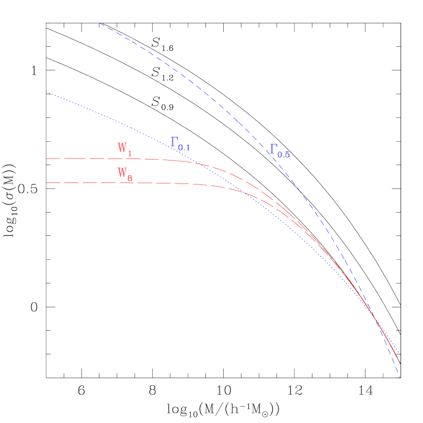
Figure 1: The $z=0$ linear amplitude of mass fluctuations for the seven models investigated in this study. $\sigma(M)$ is calculated using a top-hat real-space window function. Solid lines represent, from bottom to top, $\Lambda$CDM models $S_{0.9}$, $S_{1.2}$ and $S_{1.6}$. The short-dashed line corresponds to $\Gamma_{0.5}$ and the dotted line to $\Gamma_{0.1}$. The two WDM models are shown with long-dashed lines; the top and bottom lines correspond to models $W_{1}$ and $W_{8}$ respectively.

Table 1: Power spectrum parameter choices.

Label	$\sigma_{8}$	$\Gamma$	$M_{f}/(10^{10}{\it h}^{-1}\,{\rm M_{\odot}})$
$S_{0.9}$	$0.9$	$0.2$	-
$S_{1.2}$	$1.2$	$0.2$	-
$S_{1.6}$	$1.6$	$0.2$	-
$\Gamma_{0.1}$	$0.9$	$0.1$	-
$\Gamma_{0.5}$	$0.9$	$0.5$	-
$W_{1}$	$0.9$	$0.2$	1
$W_{8}$	$0.9$	$0.2$	8

The second power spectrum shape aims to mimic a warm dark matter (WDM) power spectrum: it is identical to the CDM spectrum on large scales but its power is reduced on scales smaller than that of a characteristic free-streaming mass, $P_{\rm WDM}(k)=P_{\rm CDM}(k)\exp(-kR_{f}-(kR_{f})^{2}))$, where $R_{f}$ is the comoving free-streaming scale. Following Sommer-Larsen & Dolgov (2000) and Avila-Reese et al. (2000), a free-streaming wavenumber, $k_{f}$, is defined as that where the WDM power spectrum is half the value for CDM. This implies $k_{f}\approx 0.46/R_{f}$. The free-streaming mass is defined as

$$M_{f}=\frac{4\pi}{3}\bar{\rho}_{\rm WDM}\left(\frac{\lambda_{f}}{2}\right)^{3},$$ (1)

with $\lambda_{f}=2\pi/k_{f}$ and $\bar{\rho}_{\rm WDM}$ being the density of WDM. Expressing the free-streaming mass in terms of the free-streaming scale yields

$$M_{f}=3.7\times 10^{14}\,\Omega_{0}\,(R_{f}/{\it h}^{-1}\,{\rm Mpc})^{3}\,{\it h}^{-1}\,{\rm M_{\odot}}.$$ (2)

This approximation to the actual WDM cosmogony neglects the non-zero velocity dispersion of the warm dark matter particle candidates, but recent work indicates that this omission should have negligible consequences for the quantities of interest here (Avila-Reese et al. 2000; Bode, Ostriker & Turok 2000). On the other hand, one advantage of this approximation is that the only difference between the CDM and WDM runs is the small-scale behavior of the power spectrum, which implies that systematic trends of halo structure with power spectrum shape are easier to identify.

Table 1 contains a list of the specific parameters chosen for the various models, and Figure 1 shows $\sigma(M)$, the $z=0$ amplitude of linear mass fluctuations in spheres of a given mass corresponding to each power spectrum. In total, seven different models were investigated; five $\Lambda$CDM models with different parameter choices for $\sigma_{8}$ and $\Gamma$ and two WDM models with different free-streaming masses, $M_{f}$. Model $S_{0.9}$ will be referred to hereafter as the ‘fiducial’ model, because it is roughly consistent with the local abundance of galaxy clusters (Eke et al. 1996) and with the amplitude of CMB fluctuations (Stompor, Gorski & Banday 1995; Liddle et al. 1996). While a value of $\Gamma=0.2$ was adopted for this default model, it is worth noting that, according to the fit of Sugiyama (1995), $\Gamma=\Omega_{0}\,h\,\exp(-\Omega_{b}-(h/0.5)^{1/2}\,(\Omega_{b}/\Omega_{0}))$, and therefore $\Gamma\approx 0.16$ would be a more appropriate value for the high baryon density parameter, $\Omega_{\rm b}\approx 0.019\,h^{-2}=0.045$ (for $h=0.65$), advocated by Tytler et al. (2000).

2.2 The Simulations

For each model listed in Table 1, the AP³M code (Couchman 1991) was used to evolve $128^{3}$ dark matter particles in a $32.5\,{\it h}^{-1}\,{\rm Mpc}$ cube from $z=24$ to $z=0$ using 2000 equal steps in expansion factor. At $z=0$, four halos with circular velocities between $180$ and $230\,{\rm km\,s^{-1}}$ (similar to that of the Milky Way) were selected for resimulation from a list of halos identified by the spherical overdensity group-finding algorithm (Lacey & Cole 1994). Unless otherwise specified, halo circular velocities, $V_{\Delta}$, are measured at the virial radius, $r_{\Delta}$; the radius of a sphere containing a mean density $\Delta$ times the critical value. The parameter $\Delta$ depends on $\Omega$ and $\Lambda$ according to (e.g. Eke, Navarro & Frenk 1998),

$$\Delta(\Omega,\Lambda)=178\cases{\Omega^{0.30},&if $\Lambda=0$;\cr\Omega^{0.45},&if $\Omega+\Lambda=1$\cr}$$ (3)

and is $\approx 100$ at $z=0$ for the cosmology adopted here. In addition to the circular velocity cuts, a criterion of relative isolation was also enforced, so that halos considered for resimulation were restricted to those without neighbors more massive than $2.7\times 10^{11}{\it h}^{-1}\,{\rm M_{\odot}}$ within $1.5\,{\it h}^{-1}\,{\rm Mpc}$. This selection criterion increases the likelihood that the selected halos are close to equilibrium, simplifying the interpretation of the results. Besides the four ‘Milky Way’ halos selected for each cosmogony, further halos extending to circular velocities of order $100\,{\rm km\,s^{-1}}$ were also selected for resimulation in the fiducial $S_{0.9}$ model and the WDM models.

The resimulations were performed using a multiple time-step N-body code based on the algorithm described by Navarro & White (1993), modified to take advantage of the GRAPE3 hardware (Sugimoto et al. 1990). Particles were allowed to take up to $86,000$ time-steps during their evolution from the starting redshift of $50$ to $z=0$. Each halo has between $35,000$ and $85,000$ particles within the virial radius at the final time. A Plummer gravitational softening of $\epsilon=0.6$ kpc was used in all resimulations of ‘Milky Way’ halos. The extra resimulated halos with $V_{\Delta}<160\,{\rm km\,s^{-1}}$ were run using $\epsilon=0.4$ kpc. A few simulations were rerun varying the numbers of particles, and indicate that this numerical setup is appropriate for making reliable measurements of the total mass within $5$-$10$ kpc.

3 Power Spectrum and Halo Concentration

3.1 CDM and WDM density profiles

Figure 2: Density profiles of dark matter halos formed in the different cosmological models. Different symbols correspond to different models, as follows: filled squares ($S_{0.9}$), stars ($S_{1.6}$), open squares ($S_{1.2}$), open circles ($\Gamma_{0.1}$), filled circles ($\Gamma_{0.5}$), filled triangles ($W_{1}$), and open triangles ($W_{8}$). Profiles shown are averages over the four ‘Milky Way’ halos ($V_{\Delta}\sim 200$ km/s) resimulated for each cosmogony. A second average halo is also shown in the lower right panel for models $S_{0.9}$, $W_{1}$ and $W_{8}$ corresponding to $V_{\Delta}\sim 100$ km/s. The curves show NFW profiles fitted to the average profiles. Line types are as in Figure 1.

Figure 2 shows the density profiles at $z=0$ corresponding to the cosmologies listed in Table 1. Each profile is an average over the four ‘Milky Way’ halos (i.e., halos with $V_{\Delta}$ in the range $180$-$230$ km/s). The mean profile for each model is shown, together with fits of the form proposed by Navarro, Frenk & White (1996, 1997, hereafter NFW),

$${\rho(r)\over\rho_{\rm crit}}={\delta_{c}\over(r/r_{s})(1+r/r_{s})^{2}},$$ (4)

where $\rho_{\rm crit}=3H^{2}/8\pi G$ is the critical density for closure, $\delta_{c}$ is a characteristic density contrast, and $r_{s}$ is a scale radius that corresponds to the region where the logarithmic slope of the density equals the isothermal value, d$\ln(\rho)/$d$\ln(r)=-2$.

The main point to note here is that the NFW fitting formula works quite well for $\Lambda$CDM halos in the radial range $0.1$-$10~{}r_{s}$, in agreement with the results of NFW. This fitting formula also reproduces the density profiles of WDM halos, even for mass scales well below the free-streaming mass, $M_{f}$. This result has been noted before (Huss, Jain & Steinmetz 1999; Avila-Reese et al. 2000; Bode et al. 2000), and allows the characterization of each halo by two simple parameters: the mass inside $r_{\Delta}$ (the virial mass $M_{\Delta}$) and the ‘concentration’ $c_{\Delta}=r_{\Delta}/r_{s}$. The concentration is directly related to the NFW characteristic density contrast by

$${\delta_{c}}={\Delta\over 3}{c_{\Delta}^{3}\over[\ln(1+c_{\Delta})-c_{\Delta}/(1+c_{\Delta})]},$$ (5)

so that either parameter describes fully the density structure of a halo of a given mass. In what follows, $c_{\Delta}$ will be adopted except in the comparison with the results of NFW, where $\delta_{c}$ will be used. This is motivated by the fact that NFW adopted $\Delta=200$ in their work, whereas the more general $\Delta$ definition of eq. 3 is adopted here. Note that $\delta_{c}$ is independent of $\Delta$, but that concentration is not, so that one should be careful when comparing concentration values quoted by different authors. For the model considered here, $\Delta\approx 100$ at $z=0$, and $c_{\Delta}\sim 1.3~{}c_{200}$. Note that, although the resolution of these simulations is good enough to measure concentrations in a robust manner, it is not adequate to address the ongoing controversy regarding the innermost slope of the density profile.

3.2 The Mass Dependence of Halo Concentration

Figure 3 shows the concentrations measured in the simulations at $z=0$, as a function of the virial mass of each halo. Different symbols correspond to different cosmogonies, as described in the caption to Figure 2. The top panel corresponds to the three $\Lambda$CDM models, $S_{1.6}$, $S_{1.2}$, and $S_{0.9}$, from top to bottom, respectively. The middle panel shows models $\Gamma_{0.5}$ and $\Gamma_{0.1}$, while the bottom panel presents results corresponding to the warm dark matter models $W_{1}$ and $W_{8}$. Results for the fiducial model $S_{0.9}$ are repeated in all panels.

Figure 3: Concentration as a function of halo mass for all models, split into three panels for ease of presentation. Lines in each panel are fits to the data using the model described in §3.3, using the same value of $C_{\sigma}=28$ (the only free parameter in the modeling) for all models. The top panel shows, from top to bottom, $\Lambda$CDM models $S_{1.6}$ (starred symbols), $S_{1.2}$ (open squares), and the fiducial model $S_{0.9}$ (filled squares). The fiducial model is repeated in all panels for comparison. The middle panel shows models $\Gamma_{0.5}$ (filled circles), and $\Gamma_{0.1}$ (open circles). The bottom panel shows $W_{1}$ (filled triangles) and $W_{8}$ (open triangles). All line types are as in Figure 1.

There are a few things to note in this figure. Firstly, $\Lambda$CDM concentrations increase with increasing $\sigma_{8}$ and decrease with increasing mass. These trends are consistent with those reported by NFW on the basis of lower resolution simulations, and support NFW’s interpretation that the concentration, or equivalently, the characteristic density of a halo, reflects the mean density of the universe at a suitably defined collapse time. Collapse redshifts increase for higher values of the normalization parameter $\sigma_{8}$, and are higher for low mass systems, reflecting the hierarchical development of structure in CDM universes.

Secondly, $\Lambda$CDM concentrations depend very weakly on mass for the range considered here; changing by only about $50\%$ over two decades in mass for model $S_{0.9}$. Figure 4 shows the simulation results presented by NFW for a variety of different cosmological models and dark matter power spectra, $P(k)$. The weak dependence on mass for the CDM models is surprising when compared with the stronger trends observed for the power-law power spectra simulations, labeled with the spectral index $n$, where $P(k)\propto k^{n}$. As $n$ becomes more negative, the concentration depends more weakly upon mass. This is to be expected, since, as pointed out by NFW, the scaling between $\delta_{c}$ and $M_{\Delta}$ found in their numerical simulation is $\delta_{c}\propto M_{\Delta}^{-(n+3)/2}$, the same that links the characteristic non-linear mass $M_{*}(z)$ and the mean cosmic density at redshift $z$. However, as can be readily seen in Figure 4, the $\delta_{c}$-$M$ dependence found for CDM models is actually much weaker than expected for $n\sim-1.5$, the ‘effective’ CDM spectral index on the mass scales probed by the NFW simulations. A more negative spectral index seems necessary to explain the CDM results. This led NFW to postulate that it is the amplitude of fluctuations on mass scales much smaller than the virial mass that determine the concentration. Consequently they introduced a (rather arbitrary) parameter of order $\mathrel{\hbox{\hbox to0.0pt{\hbox{\lower 4.0pt\hbox{$\sim$}}\hss}\hbox{$<$}}}1\%$ (see parameter $f$ in equation 7 below) in their modeling, in order to shift the mass scale under consideration and reproduce the numerical results. This is a rather unsatisfactory aspect of their modeling that lacks clear interpretation.

Figure 4: Mass dependence of halo characteristic densities, as reported by Navarro, Frenk & White (1997) (solid circles), compared with the results of the model described in §3.3. Constant $C_{\sigma}$ in eq. 13 has been chosen in each case so as to provide a good fit to the simulation results at $M_{200}\approx M_{*}$. Model SCDM corresponds to the former ‘standard’ CDM ($\Omega_{0}=1$, $\sigma_{8}=0.63$, $\Gamma=0.5$). Model CDM$\Lambda$ has $\Omega_{0}=0.25$, $\Lambda_{0}=0.75$, $\Gamma=0.19$, and $\sigma_{8}=1.3$. The rest of the panels correspond to power-law power spectra, $P(k)\propto k^{n}$; the value of $n$ and $\Omega_{0}$ is listed in each panel. Masses are normalized to the characteristic clustering mass $M_{*}$, defined so that $\sigma(M_{*})=\delta_{\rm crit}$ (=1.686 for $\Omega_{0}=1$). This corresponds to $M_{*}=1.6\times 10^{13}h^{-1}M_{\odot}$ for SCDM and $M_{*}=4.1\times 10^{13}h^{-1}M_{\odot}$ for CDM$\Lambda$. Note that excellent fits can be obtained in all cases with similar values of the single free parameter $C_{\sigma}$.

Finally, further clues can be gleaned from the concentration of $\Gamma_{0.5}$ and $\Gamma_{0.1}$ halos. $\Gamma_{0.1}$ concentrations are lower than $S_{0.9}$, which is not surprising given that the amplitude of mass fluctuations is significantly lower on galactic scales (Figure 1). On the other hand, $\Gamma_{0.5}$ concentrations are as high as $S_{1.6}$, although $\sigma(M)$ is in this case lower than $S_{1.6}$ on galaxy-mass scales (Figure 1). This again hints that the amplitude on virial mass scales is a poor predictor of the concentration. These hints are confirmed by the results of WDM model $W_{8}$, which shows a clear reversal of the concentration versus mass trend on scales below a few times the free-streaming mass $M_{f}$. $W_{8}$ concentrations decrease with decreasing mass despite the fact that WDM $\sigma(M)$ increases towards low masses before saturating at $M\ll M_{f}$ (Figure 1).

3.3 A model for the power spectrum dependence of the concentration

Although the model proposed by NFW captures many of the qualitative trends shown in Figure 3 it suffers from two main shortcomings: (i) it introduces two arbitrary parameters whose interpretation remains unclear, and (ii) it predicts a redshift dependence for the concentration that is weaker than found in recent numerical simulations (Bullock et al. 2000). Bullock et al. propose an alternative prescription, also with two free parameters, that results in improved agreement between the predicted redshift dependence of concentrations and the results of the numerical simulations. Their model follows NFW in associating a halo’s characteristic density with the average background density at collapse time, but differs from NFW in the definition of characteristic density and collapse time.

More specifically, NFW take the characteristic density of a halo to be $\delta_{c}$ (see eq. 5), and use a constant of proportionality, $C$, to relate this to the mean background density at the collapse redshift, $z_{c}$, according to

$$\delta_{c}=C\,\Omega_{0}\,(1+z_{c})^{3}.$$ (6)

The collapse time is defined as that when, according to the Press & Schechter approach (Press & Schechter 1974; Lacey & Cole 1993) , half the virial mass of the halo was first contained in progenitors more massive than a fraction $f$ of the final mass. This implies that

$${\rm erfc}\left\{\frac{\delta_{\rm crit}(z_{c})-\delta_{\rm crit}(z_{o})}{\sqrt{2[\sigma^{2}(fM)-\sigma^{2}(M)]}}\right\}=\frac{1}{2},$$ (7)

where $z_{o}$ denotes the redshift at which the halo is identified, $\delta_{\rm crit}(z)=\delta_{\rm crit}(0)/D(z)$ is the spherical top-hat model linear overdensity threshold and $D(z)$ represents the linear theory growth factor. ($D(z)=(1+z)^{-1}$ if $\Omega_{0}=1$, $\Lambda_{0}=0$ is conventionally normalized to unity at $z=0$; formulae for other values of $\Omega_{0}$ and $\Lambda_{0}$ can be found in Peebles 1980.) For their simulations, NFW found a good fit by adjusting the two free parameters to be $C=3000$ and $f=0.01$.

Bullock et al., on the other hand, choose the characteristic density, ${\tilde{\rho}}_{s}$, to be such that

$$M_{\Delta}={4\pi\over 3}r_{s}^{3}\,{\tilde{\rho}}_{s},$$ (8)

and specify the collapse redshift, $z_{c}$, solely in terms of $\sigma(M)$, so that

$$D(z_{c})\,\sigma(F\,M_{\Delta})=1.686,$$ (9)

where $F=0.01$. Their second free parameter, $K$, relates the characteristic density to the background density via

$${\tilde{\rho}}_{s}=K^{3}\Delta(z_{o})\rho_{\rm crit}(z_{c})$$ (10)

and feeds through into the concentration as

$$c_{\Delta}=K\left(\frac{1+z_{c}}{1+z_{o}}\right).$$ (11)

$K=4$ provides a good fit to their $\Lambda$CDM simulation results.

This model, like that of NFW, suffers from the introduction of two arbitrary parameters ($F$ and $K$) whose interpretation remains unclear. Furthermore, the definition of collapse epoch given in equation 9 implies that for a truncated power spectrum such as WDM, halo concentrations will still increase monotonically with decreasing mass, approaching a constant at $M\ll M_{f}$. This is at odds with the results presented in the previous section (see also Bode et al. 2000), which show that WDM halo concentrations decrease on mass scales below a few times the free-streaming mass. These results strongly suggest that it is not only the amplitude of the power spectrum, but also its shape, that determine the concentration of dark matter halos. In particular, only a modeling that includes such shape dependence will be able to reproduce the somewhat counterintuitive dependence of concentration on halo mass found for truncated power spectra such as $W_{8}$ (see Figure 3).

After some experimentation, a simple model has been produced that matches the mass dependence of halo concentrations for the simulations presented here. Furthermore, the same model also fits all of the original NFW results, whilst modifying the redshift dependence of concentrations so that they are compatible with the recent results of Bullock et al. The new model has a single free parameter and is of more general applicability, since it can be applied to truncated power spectra, where Bullock et al.’s prescription fails. This model also removes the need for the arbitrary, small mass fraction constant introduced by NFW and Bullock et al. (f=0.01 in equation 7 and F=0.01 in equation 9) by postulating that the concentration of a halo is controlled by a combination of the amplitude and shape of the power spectrum.

Consider the ‘effective’ amplitude of the power spectrum on scale $M$, defined by,

$$\sigma_{\rm eff}(M)=\sigma(M)\,\left(-{{\rm d}\ln(\sigma)\over{\rm d}\ln(M)}(M)\right).$$ (12)

This effective amplitude modulates $\sigma(M)$ so that, for WDM-like spectra, it decreases on mass scales smaller than a few times the free-streaming mass $M_{f}$. In broad terms, a given mass scale $M$ collapses when $D(z)\sigma(M)$ is at least unity. This time is controlled by the redshift evolution of the linear growth factor, $D(z)$, appropriate for the cosmological model under consideration. Following this, the collapse redshift, $z_{c}$, of a halo of mass $M$ may be identified as

$$D(z_{c})\sigma_{\rm eff}(M_{s})={1\over C_{\sigma}}$$ (13)

where $C_{\sigma}$ is a constant and $M_{s}$ is the mass contained within $r_{\rm max}=2.17\,r_{s}$, the radius at which the circular velocity of an NFW halo reaches its maximum. The requirement for collapse that $D(z_{c})\sigma(M_{s})\geq 1$ implies that $C_{\sigma}\geq-{\rm d}\ln\sigma/{\rm d}\ln M$. For a power-law fluctuation spectrum with $P(k)\propto k^{n}$ then this yields $C_{\sigma}\geq 6/(n+3)$. As in the models of NFW and Bullock et al., the mean density of the universe at the collapse redshift can then be used to calculate a characteristic density for the halo. Defining the characteristic density of the halo to be, as in Bullock et al. (see eq. 8),

$${\tilde{\rho}}_{s}=\Delta(z_{o})\,\rho_{\rm crit}(z_{o})\,c_{\Delta}^{3},$$ (14)

and setting this to equal the spherical collapse top-hat density at the collapse epoch, $\rho_{\rm sc}$, where

$$\rho_{\rm sc}(z_{c})=\Delta(z_{c})\rho_{\rm crit}(z_{c})=\Delta(z_{c})\frac{\bar{\rho}_{0}(1+z_{c})^{3}}{\Omega(z_{c})}$$ (15)

yields,

$$c_{\Delta}^{3}={\Delta(z_{c})\over\Delta(z_{o})}\,{\Omega(z_{o})\over\Omega(z_{c})}\,\left({1+z_{c}\over 1+z_{o}}\right)^{3}.$$ (16)

Equations 13 and 16 describe the concentration of a halo of given mass, once the single free parameter in eq. 13, $C_{\sigma}$, has been specified. As the characteristic mass scale at which the effective amplitude of the power spectrum is evaluated depends on $r_{s}$, and therefore on $c_{\Delta}$, equations 13 and 16 need to be solved iteratively to yield the combination of $c_{\Delta}$ and $z_{c}$ .

This model reproduces, with roughly the same value of $C_{\sigma}$, the results of the simulations presented here, all of the original results of NFW, as well as the redshift dependence advocated by Bullock et al. This is shown by the curves in Figure 3, which show the result of applying the model, at $z=0$, to the seven cosmogonies adopted in this study. Solid line types are used for the $S$ models, short-dashed and dotted lines for $\Gamma_{0.5}$ and $\Gamma_{0.1}$, respectively, while long-dashed lines are used for WDM. All of the curves use the same value for the proportionality constant in eq. 13, $C_{\sigma}=28$. The model reproduces very well the trends with mass, normalization, and shape of the power spectrum seen here, including the counterintuitive trend towards lower concentrations seen in the low-mass $W_{8}$ halos. Table 2 contains a list of concentrations for a $10^{12}{\it h}^{-1}\,{\rm M_{\odot}}$ halo identified at $z=0$ in a variety of commonly studied cosmological models. This illustrates the interplay between $\Omega_{0}$, $\Lambda_{0}$, $\sigma_{8}$ and $\Gamma$.

Table 2: Values of $c_{\Delta}$ and $c_{200}$ for a $10^{12}{\it h}^{-1}\,{\rm M_{\odot}}$ halo identified at $z=0$ in four commonly studied cosmological models.

$\Omega_{0}$	$\Lambda_{0}$	h	$\sigma_{8}$	$\Gamma$	$c_{\Delta}$	$c_{200}$
$1$	$0$	$0.5$	$0.5$	$0.5$	$12.3$	$11.7$
$1$	$0$	$0.5$	$0.5$	$0.2$	$6.7$	$6.4$
$0.3$	$0$	$0.65$	$0.9$	$0.2$	$18.6$	$15.2$
$0.3$	$0.7$	$0.65$	$0.9$	$0.2$	$12.0$	$8.9$

The model described above also reproduces the original results of NFW quite well. This is shown in Figure 4, where the density contrast $\delta_{c}$ is plotted as a function of the mass enclosed within a $\Delta=200$ sphere, the parameters used by NFW. It is apparent from this figure that the model also reproduces the results of the eight cosmogonies studied by NFW, including open models with $\Omega_{0}$ as low as $0.1$, again with approximately a single value of the constant $C_{\sigma}$.

3.4 The Redshift Dependence of Halo Concentration

According to equations 13 and 16, the model predicts that, at fixed halo mass, in an Einstein-de Sitter cosmogony $c_{\Delta}(M,z)\propto(1+z)$. This relation agrees with the prediction of the model by Bullock et al. for the evolution of halo concentration. However, for low density universes the scaling with redshift is not the same as theirs, and it is therefore important to verify that it is still in good agreement with the numerical results.

Figure 5: Comparison between concentrations measured at $z=0$ (left panels) and $z=2$ (right panels), and the predictions of three different models. ‘ENS’ corresponds to the model presented in this paper (top panels), ‘B’ to that in Bullock et al (2000, middle panels), and ‘NFW’ to concentrations computed using the procedure outlined in the Appendix of NFW (bottom panels). The filled-in squares correspond to $S_{0.9}$ halos, whereas open triangles correspond to $W_{8}$ halos. The solid and dashed curves show the model predictions for $S_{0.9}$ and $W_{8}$, respectively.

Figure 5 compares the predictions of all three different concentration models with the results of the numerical simulations at $z=0$ and $2$. The comparison includes all halos in the $S_{0.9}$ and $W_{8}$ simulations with more than $2500$ particles within $r_{\Delta}$. Concentrations labelled with an ‘ENS’ subscript in the top row correspond to the model presented here, ‘B’ to Bullock et al.’s (middle row), and ‘NFW’ for the NFW model predictions in the bottom panels. ENS concentrations use $C_{\sigma}=28$ in eq. 13. ‘B’ concentrations use $F=0.01$ and $K=4$. NFW concentrations use $C=3000$ and $f=0.01$. The typical halo mass range probed varies from $10^{11}$-$10^{13}{\it h}^{-1}\,{\rm M_{\odot}}$ at $z=0$ to $10^{10.5}$-$10^{12}{\it h}^{-1}\,{\rm M_{\odot}}$ at $z=2$.

The top two panels show that the model presented here predicts a redshift dependence in good agreement with the simulation results, both for $S_{0.9}$ and $W_{8}$. The middle panels show that the Bullock et al. model also fits the results of the fiducial $\Lambda$CDM runs at $z=0$ and $z=2$, but that their model fails to capture the mass dependence seen in the $W_{8}$ simulations. This illustrates the point that was made earlier that it is the effective normalization (equation 12), rather than simply $\sigma(M)$, that determines halo concentrations. The bottom row highlights the weak redshift dependence predicted by the NFW model compared with the simulation results, as noted by Bullock et al.; it slightly under-predicts the fiducial model concentrations at $z=0$ but over-predicts them at $z=2$.

In summary, the data in Figure 5 shows that the redshift evolution predicted by the model presented here is consistent with the simulation results. Even at $z=5$, the highest redshift with simulation data in figure 11 of Bullock et al., the concentrations of $10^{12}{\it h}^{-1}\,{\rm M_{\odot}}$ halos are $c_{\Delta}=2.6$ and $2.5$ for the model in Section 3.3 and that of Bullock et al. respectively. Thus, it is not possible to discriminate between the slightly different redshift dependences of these two models.

4 Comparison with Observations

4.1 $\Lambda$CDM and the Dark Mass within the Solar Circle

Observations of star and gas kinematics provide well defined constraints on the dark matter content of the Milky Way within the solar circle, $R_{0}=8.5$ kpc. As discussed by NS00a (see that paper for full references), a simple upper limit on the dark mass within $R_{0}$, $M_{\rm dark}(r<R_{0})$, may be obtained by combining the observed circular velocity at the Sun’s location, $V_{c}(R_{0})=220\,{\rm km\,s^{-1}}$, with estimates for the total mass and exponential scalelength of the Galactic disk ($M_{\rm disk}=6\times 10^{10}M_{\odot}$ and $r_{\rm disk}=3.5$ kpc, respectively). The result (note that there is a typo in eq.1 of NS00a),

$$M_{\rm dark}(r<R_{0})\mathrel{\hbox{\hbox to0.0pt{\hbox{\lower 4.0pt\hbox{$\sim$}}\hss}\hbox{$<$}}}4.3\times 10^{10}M_{\odot},$$ (17)

constitutes an upper limit because the simple calculation described above neglects two potentially important effects: (i) the contribution of the bulge, and (ii) any potential contraction that the dark halo may have experienced as a result of the assembly of the galaxy.

Figure 6: Dark matter halo masses within the solar circle ($8.5$ kpc) compared with constraints derived from dynamical observations of the Milky Way (hatched region). A vertical arrow marks a circular velocity of $220~{}{\rm km\,s^{-1}}$. The different symbols correspond to different cosmogonies, as specified in Figure 2. Lines correspond to NFW profiles assuming concentrations given by the model in §3.3.

The constraint expressed in eq. 17 is straightforward to compare with the results of the numerical simulations described here. This is done in Figure 6, where the dark mass within $8.5$ kpc is plotted as a function of $V_{200}$, the halo circular velocity for $\Delta=200$ used in NS00a, for all of the halos. The top panel shows halos formed in the $S_{0.9}$, $S_{1.2}$, and $S_{1.6}$ models, the three different normalizations chosen for the $\Lambda$CDM scenario. At $V_{200}=220\,{\rm km\,s^{-1}}$ (marked with an arrow in Figure 6), $M_{\rm dark}(r<R_{0})$ increases approximately in proportion to $\sigma_{8}$. In light of the modeling described above, this can be attributed to the higher average collapse times that result from the choice of higher normalizations.

The lines in this panel correspond to the mass within $8.5$ kpc predicted by the model described in §3.3. Combining this model with the constraint in eq. 17 it is possible to estimate the range of circular velocities allowed for the halo of the Milky Way as a function of the normalization parameter $\sigma_{8}$:

$$\sigma_{8}\,v_{220}\,m_{\rm dark}<0.8,$$ (18)

where $v_{220}$ is the circular velocity, $V_{200}$, of the Milky Way halo in units of $220\,{\rm km\,s^{-1}}$, and $m_{\rm dark}$ is $M_{\rm dark}/(4.3\times 10^{10}M_{\odot})$. This suggests that, for $\Gamma=0.2$, the circular velocity of the halo of the Milky Way should be somewhat less than $220\,{\rm km\,s^{-1}}$, unless $\sigma_{8}<0.9$ or the Milky Way halo has an unusually low concentration for its mass. The fiducial $S_{0.9}$ model may be reconciled with the Milky Way constraint if $V_{200}\mathrel{\hbox{\hbox to0.0pt{\hbox{\lower 4.0pt\hbox{$\sim$}}\hss}\hbox{$<$}}}195\,{\rm km\,s^{-1}}$. A knock-on effect of moving the Milky Way into a smaller halo would be that any predictions of the galaxy luminosity function made by mapping mass into luminosity using the properties of the Milky Way would find that Milky Way-type galaxies were more abundant than before. As $M\propto V^{3}$, and assuming that the luminosity of a galaxy is proportional to its mass, it only takes a $20\%$ decrease in halo circular velocity to halve the luminosity. Thus, it remains to be seen whether assigning the luminosity of the Milky Way to the many halos with $V_{200}\approx 195\,{\rm km\,s^{-1}}$ is consistent with the luminosity function of bright spirals (see, e.g., Cole et al. 1994; Cole et al. 2000).

A lower bound on the mass of the Milky Way halo may be derived by requiring that the total baryonic mass of the Galaxy does not exceed the baryon mass within the virial radius of the halo. Assuming $\Omega_{b}=0.019\,h^{-2}\approx 0.045$, the minimum halo mass corresponds to a circular velocity of $\sim 105\,{\rm km\,s^{-1}}$. This is lower than the $130\,{\rm km\,s^{-1}}$ derived by NS00a, because of the lower baryon fraction ($\Omega_{b}=0.0125h^{-2}$) and slightly higher Hubble constant ($h=0.7$) adopted by those authors.

From Figure 6, halos in the fiducial $S_{0.9}$ $\Lambda$CDM model with circular velocities in the range $(105,190)\,{\rm km\,s^{-1}}$ appear consistent with the Milky Way constraint. For $\sigma_{8}=1.2$ the range of acceptable halo masses is narrower, and essentially no halo agrees with the observational constraints if $\sigma_{8}=1.6$. This is reminiscent, although less stringent, than the conclusion reached by NS00a, who argued that $\sigma_{8}=1.14$ $\Lambda$CDM halos were too concentrated to be consistent with this constraint. However, a reanalysis of the NS00a dataset reveals that because of inconsistencies in the normalization procedure for their $\Lambda$CDM simulations , those authors had effectively normalized their power spectra to $\sigma_{8}\sim 1.6$ rather than $\sigma_{8}=1.14$. After correcting for this error, the results in NS00a,b are consistent with those reported here.

4.2 The zero-point of the Tully-Fisher relation

As discussed by NS00a,b, the analysis of Section 4.1 can be extended to other spiral galaxies by examining the correlation between galaxy luminosity and the rotation speed of their gas and stars: the Tully-Fisher relation (Tully & Fisher 1977). Provided that stellar mass-to-light ratios and exponential scalelengths can be estimated reliably, it is possible to evaluate the disk contribution to the circular velocity at $2.2$ exponential scalelengths (where the disk contribution peaks and optical Tully-Fisher velocities are typically measured) and derive constraints on the total dark mass contained within this radius.

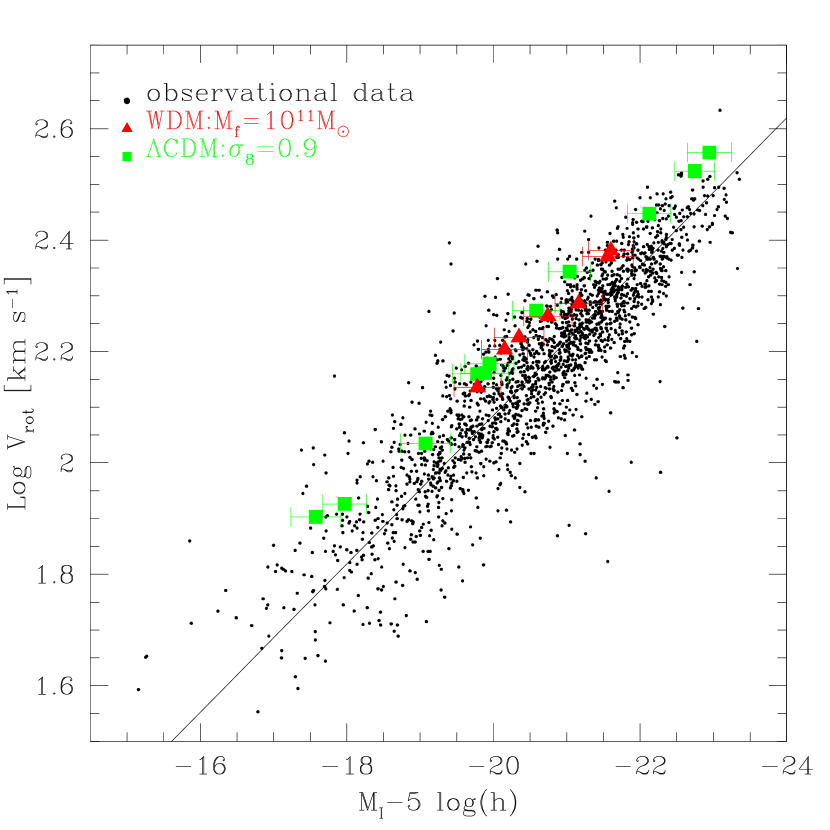
Figure 7: The I-band Tully-Fisher relation compared to the result of numerical simulations in the fiducial $\sigma_{8}=0.9$ $\Lambda$CDM (filled squares) and in the $W_{1}$ warm dark matter (filled triangles) scenarios. Dots are a compilation of the data by Giovanelli et al (1997), Mathewson et al (1992), and Han & Mould (1992). The solid line is the best fit to the data advocated by Giovanelli et al. Horizontal ‘error bars’ in the simulation results span the range in luminosities derived from assuming a Scalo or a Salpeter IMF. Simulation circular velocities are measured at $r_{\rm gal}=20(V_{200}/220\,{\rm km\,s^{-1}})\,{\it h}^{-1}\,{\rm kpc}$. Note that the slope, scatter and zero-point of the numerical TF relation are all in reasonable agreement with observation.

The more concentrated a halo is, the faster a disk of given mass and radial scale must rotate to attain centrifugal equilibrium. Thus, as shown by NS00a,b, the zero-point of the Tully-Fisher relation provides a direct constraint on halo concentrations. Although these authors conclude that $\sigma_{8}=1.14$ $\Lambda$CDM halos are too concentrated to be consistent with the I-band Tully-Fisher relation, as discussed in §4.1 their conclusions were affected by an inconsistent normalization of the power spectrum. Given that the simulations of NS00a,b effectively probed a $\sigma_{8}\approx 1.6$ $\Lambda$CDM model and concentration depends strongly on $\sigma_{8}$, it is appropriate to revisit the issue and verify whether the fiducial $S_{0.9}$ model is consistent with observations.

4.2.1 Gasdynamical simulations

To this aim, a number of gasdynamical simulations including star formation and feedback have been run using GRAPESPH, a code that combines the hardware N-body integrator GRAPE with the smoothed-particle hydrodynamics (SPH) technique (Steinmetz 1996). The simulation setup and analysis are identical to those described in Navarro & Steinmetz (1997) and Steinmetz & Navarro (1999), and the reader is referred there for details. In brief, the same initial conditions described above for the dark matter-only runs are used with the addition of gas, assuming a value of $\Omega_{b}=0.0125h^{-2}$ for the baryon density parameter. Models with gas have typically $20,000$ gas particles and the same number of dark matter particles. Up to $5,000$ of these end up in a galaxy at $z=0$, resulting in lower resolution than the N-body simulations discussed in previous sections. Gas particle masses range from $4.5\times 10^{6}M_{\odot}$ to $2.5\times 10^{8}M_{\odot}$, depending on the model considered.

Model galaxies are unmistakably identified in the runs as star and gas clumps with high density contrast. Only halos with more than $500$ dark particles within the virial radius have been retained for analysis. The properties of the luminous component are computed within a radius, $r_{\rm gal}=20\,(V_{200}/220\,{\rm km\,s^{-1}}){\it h}^{-1}\,{\rm kpc}$. This radius contains all of the baryonic material associated with the galaxy and is well outside the region compromised by numerical resolution effects. All of the rotation speeds are also computed at that radius. Note that $r_{\rm gal}$ exceeds the radii at which Tully-Fisher velocities are typically measured, but given the lower resolution of these simulations, rotation speeds at smaller radii are quite uncertain. This comparison therefore assumes that the circular velocity curves of actual disk galaxies remain approximately flat out to $r_{\rm gal}$.

4.2.2 The I-band TF relation

Figure 7 compares the observed I-band Tully-Fisher relation (dots) with the numerical results for galaxies selected in the fiducial $S_{0.9}$ $\Lambda$CDM model (filled squares) and in the $W_{1}$ WDM model. There is reasonable agreement between observation and simulations. The slope of the numerical TF relation is consistent with the observed value, and the scatter is much smaller ($0.12$ mag rms for $S_{0.9}$ and $0.10$ mag rms for $W_{1}$) than observed. These two conclusions are in agreement with the results of NS00a,b.

The main difference with that work is that now even the zero-point of the numerical relation appears to match reasonably well the observed value; the zero-point offset between simulations and observations is $\sim 0.5$ mag, compared with the $1.5$ mag offset reported by NS00a,b. The reason for the discrepancy can again be traced to the lower concentrations of $S_{0.9}$ halos compared with the results of NS00a,b. Figure 7 also shows that there is little difference in the TF results obtained for $W_{1}$ or $S_{0.9}$, supporting the interpretation that the halo concentration is the main factor responsible for the zero-point of the numerical TF relation.

The $0.5$ mag difference between simulation and observation is not too worrying given that the simulated galaxies have colors that are slightly too red compared with their TF counterparts. The average $B-R$ color of the simulated galaxies is $1.2$, with little dependence on luminosity. For comparison, the average $B-R$ in Courteau’s (1997) sample is $\sim 0.8$. This suggests that star formation in the simulations occurs too early. Any modification to the feedback algorithm that remedies this will also tend to make the stellar population mix in the simulated galaxies brighter. If this correction can bring the stellar I-band mass-to-light ratios down from $2.5$ to $1.5$, a value more in keeping with the results of Bell & de Jong (2000), then the $0.5$ mag gap should be possible to bridge.

In summary, it appears that if the I-band stellar mass-to-light ratio of TF galaxies is of order $(M/L)_{I}\approx 1.5$ then $\Lambda$CDM halos are consistent with the slope, scatter and zero-point of the I-band Tully-Fisher relation. Note however, that while halos formed in the fiducial $\Lambda$CDM scenario appear to have concentrations consistent with observational constraints, other problems associated with the assembly of disk galaxies through merging persist. In particular, the angular momentum (and size) of simulated disks is still quite below observed values, again suggesting that perhaps the feedback algorithm is not effective enough at preventing the early collapse of baryons into protogalactic potential wells (Navarro & Steinmetz 1997). Accounting simultaneously for the luminosity, velocity, and angular momentum of spiral galaxies in these models remains a challenging problem for the $\Lambda$CDM cosmogony.

5 Summary and Conclusions

This paper contains the results from an extensive suite of numerical simulations which were aimed at understanding the relationship between the power spectrum of initial density fluctuations and the concentration of virialized dark matter halos. These simulations demonstrate that dark halo concentration depends both on the amplitude of mass fluctuations as well as on the shape of the power spectrum. A simple model that takes this into account by defining an effective amplitude as $\sigma(M)$ times the logarithmic derivative of $\sigma(M)$ with respect to mass on scales similar to the characteristic mass of the halo (i.e. that enclosed within the radius where the circular velocity peaks, $r_{\rm max}=2.17\,r_{s}$) has been developed. This model reproduces the mass and redshift dependence of the concentration in all 7 cosmogonies investigated here, as well as in the 8 different cosmogonies probed by NFW. It also extends the earlier models of NFW and Bullock et al. (2000) to power spectra very different from CDM, including truncated power spectra such as those appropriate for WDM.

These findings are applied to the Milky Way, where observational limits on the dark mater content within the solar circle can be turned into constraints on the shape and normalization of the power spectrum. For the popular $\Lambda$CDM spectrum, the Milky Way halo mass and the normalization of the power spectrum must satisfy the condition, $\sigma_{8}\,v_{220}\,m_{\rm dark}<0.8$, where $v_{220}$ is the circular velocity of the halo ($V_{200}$) in units of $220\,{\rm km\,s^{-1}}$ and $m_{\rm dark}$ is the upper limit on the mass of dark matter within $8.5$ kpc of the middle of the Milky Way in units of $4.3\times 10^{10}M_{\odot}$. For $\sigma_{8}=0.9$, the normalization favored from the abundance of galaxy clusters and CMB studies, this implies that the Milky Way halo has a circular velocity significantly smaller than the rotation speed at the solar circle, $V_{200}<195\,{\rm km\,s^{-1}}$. This finding may have significant impact on the luminosity function expected in this model, since $195\,{\rm km\,s^{-1}}$ halos are much more abundant than their $220\,{\rm km\,s^{-1}}$ counterparts (see, e.g., Cole et al. 1994, 2000). Gasdynamical simulations including star formation and feedback also show that, because of their lower concentration relative to the NS00a,b study, $\Lambda$CDM halos are also roughly consistent with the zero-point of the I-band Tully-Fisher relation. The slope and scatter of this relation is also in good agreement with observed values.

Halo concentrations in $\Lambda$CDM simulations are much lower than found by NS00a,b, who had argued that $\Lambda$CDM halos were too concentrated to be consistent with observations of the dynamics of spiral galaxies. A reanalysis of their dataset reveals an inconsistency in the normalization of the power spectrum used in that work. Instead of the intended $\sigma_{8}=1.14$, their simulations had an effective normalization of $\sigma_{8}\approx 1.6$. Once this correction is taken into account both studies yield consistent results.

The set of simulations reported here thus identify and illustrate the tight relation between power spectrum and halo concentrations. The application of these results to the Milky Way and I-band Tully-Fisher relation lifts previous concerns and suggests that the concentration of $\sigma_{8}=0.9$ $\Lambda$CDM halos is not clearly incompatible with observations.

References

- (1) Avila-Reese V., Colin P., Valenzuela O., D’Onghia E., Firmani C., 2000, ApJ, submitted (astro-ph/0010525)
- (2) Bardeen J.M., Bond J.R., Kaiser N., Szalay A.S., 1986, ApJ, 304, 15
- (3) Bell E.F., de Jong R.S., 2001, ApJ, accepted (astro-ph/0011493)
- (4) Bullock J.S., Kolatt T.S., Sigad Y., Somerville R.S., Kravtsov A.V., Klypin A.A., Primack J.R., Dekel A., 2000, MNRAS, accepted (astro-ph/9908159)
- (5) Carollo C.M., de Zeeuw P.T., van der Marel R.P., Danziger I.J., Qian E.E., 1995, ApJ, 441, L25
- (6) Cole S., Aragon-Salamanca A., Frenk C.S., Navarro J.F., Zepf S.E., 1994, MNRAS, 271, 781
- (7) Cole S., Lacey C., Baugh C.M., Frenk C.S., 2000, MNRAS, 319, 168
- (8) Couchman H.M.P., 1991, ApJ, 368, L23
- (9) Cretton N., Rix H.-W., de Zeeuw P.T., 2000, ApJ, 536, 319
- (10) Dehnen W., Binney J.J., 1998, MNRAS, 294, 429
- (11) Eke V.R., Cole S., Frenk C.S., 1996, MNRAS, 282, 263
- (12) Eke V.R., Navarro J.F., Frenk C.S., 1998, ApJ, 503, 569
- (13) Flores R.A., Primack J.R., Blumenthal G.R., Faber S.M., 1993, ApJ, 412, 443
- (14) Flores R.A., Primack J.R., 1994, ApJ, 427, L1
- (15) Frenk C.S., White S.D.M., Davis M., Efstathiou G., 1988, ApJ, 327, 507
- (16) Gerhard O., 2000, to appear in Galaxy Disks and Disk Galaxies, ASP Conference Series, J.G. Funes, S.J., and E.M. Corsini, eds (astro-ph/0010539)
- (17) Gerhard O., Jeske G., Saglia R.P., Bender R., 1998, MNRAS, 295, 197
- (18) Hogan C.J., Dalcanton J.J., 2000, Phys. Rev. D, submitted (astro-ph/0002330)
- (19) Hu W., Barkana R., Gruzinov A., 2000, Phys. Rev. Lett., submitted (astro-ph/0003365)
- (20) Huss A., Jain B., Steinmetz M., 1999, MNRAS, 308, 1011
- (21) Klypin A.A., Kravtsov A.V., Bullock J.S., Primack J.R., 2000, ApJ, submitted (astro-ph/0006343)
- (22) Klypin A.A., Kravtsov A.V., Valenzuela O., Prada F., 1999, ApJ, 522, 82
- (23) Kravtsov A.V., Klypin A.A., Bullock J.S., Primack J.R., 1998, ApJ, 502, 48
- (24) Kronawitter A., Saglia R.P., Gerhard O., Bender R., 2000, A&AS, 144, 53
- (25) Lacey C., Cole S., 1993, MNRAS, 262, 627
- (26) Lacey C., Cole S., 1994, MNRAS, 271, 676
- (27) Liddle A.R., Lyth D.H., Viana P.T.P., White M., 1996, MNRAS, 282, 281
- (28) McGaugh S.S., de Blok W.J.G., 1998, ApJ, 499, 41
- (29) Moore B., 1994, Nature, 370, 629
- (30) Moore B., Governato F., Quinn T., Stadel J., Lake G., 1998, ApJ, 499, L5
- (31) Moore B., Ghigna S., Governato F., Lake G., Quinn T., Stadel J., Tozzi P., 1999a, ApJ, 524, L19
- (32) Moore B., Quinn T., Governato F., Stadel J., Lake G., 1999b, MNRAS, 310, 1147
- (33) Navarro J.F., White S.D.M., 1993, MNRAS, 265, 271
- (34) Navarro J.F., Frenk C.S., White S.D.M., 1996, ApJ, 462, 563
- (35) Navarro J.F., Frenk C.S., White S.D.M., 1997, ApJ, 490, 493
- (36) Navarro J.F., Steinmetz M., 1997, ApJ, 478, 13
- (37) Navarro J.F., Steinmetz M., 2000, ApJ, 528, 607 (NS00a)
- (38) Navarro J.F., Steinmetz M., 2000, ApJ, 538, 477 (NS00b)
- (39) Peebles P.J.E., 1980, The Large Scale Structure of the Universe. Princeton Univ. Press, Princeton, NJ
- (40) Peebles P.J.E., 2000, ApJ, 534, L127
- (41) Press W.H., Schechter P., 1974, ApJ, 187, 425
- (42) Rix H.-W., de Zeeuw P.T., Cretton N., van der Marel R.P., Carollo C.M., 1997, ApJ, 488, 702
- (43) Sommer-Larsen J., Dolgov A., 2000, ApJ, submitted (astro-ph/9912166)
- (44) Spergel D.N., Steinhardt P.J., 2000, Phys. Rev. Lett., 84, 3760
- (45) Steinmetz M., 1996, MNRAS, 278, 1005
- (46) Steinmetz M., Navarro J.F., 1999, ApJ, 513, 555
- (47) Stompor R., Gorski K.M., Banday A.J., 1995, MNRAS, 277, 1225
- (48) Sugimoto D., Chikada Y., Makino J., Ito T., Ebisuzaki T., Umemura M., 1990, Nat, 345, 33
- (49) Sugiyama N., 1995, ApJS, 100, 281
- (50) Swaters R.A., 1999, Ph.D. thesis, Rijksuniversiteit Groningen
- (51) Swaters R.A., Madore B.F., Trewhella M., 2000, ApJ, 531, L107
- (52) Tully R.B., Fisher J.R., 1977, A&A, 54, 661
- (53) Tytler D., O’Meara J.M., Suzuki N., Lubin D., 2000, Physica Scripta, 85, 12
- (54) van den Bosch F.C., Robertson B.E., Dalcanton J.J., de Blok W.J.G., 2000, AJ, 119, 1579
- (55) van den Bosch F.C., Swaters R.A., 2000, AJ, submitted, (astro-ph/0006048)