FEEDBACK FROM GALAXY FORMATION: PRODUCTION AND PHOTODISSOCIATION OF PRIMORDIAL H₂

Abstract

We use 1D radiative transfer simulations to study the evolution of H₂ gas-phase (H^- catalyzed) formation and photo-dissociation regions in the primordial universe. We find a new positive feedback mechanism capable of producing shells of H₂ in the intergalactic medium, which are optically thick in some Lyman-Werner bands. While these shells exist, this feedback effect is important in reducing the H₂ dissociating background flux and the size of photo-dissociation spheres around each luminous object. The maximum background opacity of the IGM in the H₂ Lyman-Werner bands is $\tau_{H_{2}}\approx 1-2$ for a relic molecular fraction $x_{H_{2}}=2\times 10^{-6}$, about 6 times greater than found by Haiman et al. (2000). Therefore, the relic molecular hydrogen can decrease the photo-dissociation rate by about an order of magnitude. The problem is relevant to the formation of small primordial galaxies with masses $M_{DM}\lesssim 10^{8}$ M_⊙, that rely on molecular hydrogen cooling to collapse. Alternatively, the universe may have remained dark for several hundred million years after the birth of the first stars, until galaxies with virial temperature $T_{vir}\gtrsim 10^{4}$ K formed.

1 Introduction

Many recent observations point to a flat geometry and a significant cold dark matter (CDM) content. Recent measurements of the Cosmic Microwave Background (CMB) anisotropies (de Bernardis et al., 2000; Lange et al., 2001; Tegmark et al., 2000), large-scale structure (Hamilton & Tegmark, 2000), Ly$\alpha$ power spectrum (Croft et al., 1999; McDonald et al., 2000), and distances of high redshift SNe (Perlmutter et al., 1998; Riess et al., 1998; Garnavich et al., 1998) are all consistent with a flat CDM model of the universe, in which about 1/3 the total energy density of the universe is dark matter (DM) and 2/3 is “vacuum energy”. Big-Bang nucleosynthesis fits to the observed $D/H$ abundances suggest a small baryon density, with closure parameter $\Omega_{b}h^{2}\sim 0.02$ (Burles & Tytler, 1998). Thus, the baryons are a small fraction of the DM. In the linear phase of structure formation, the baryons simply trace the DM perturbations on large scales.

In CDM cosmologies, small mass DM virialized objects form first. Larger halos form later from the merger of smaller subunits (hierarchical scenario). Since the gas temperature prior to reionization is about 100 K, the gas can collapse in objects with M${}_{DM}>10^{4}-10^{5}$ M_⊙. Small mass DM halos will then produce the first luminous objects (Pop III) if the baryons collapsed into the DM potential wells and heated to the virial temperature can dissipate their internal energy support. The lack of metals in the primordial universe makes molecular hydrogen the only coolant below $T\sim 10^{4}$ K. Therefore, unless some H₂ is formed, the baryons can not cool in shallow DM potential wells with M${}_{DM}\lesssim 10^{8}[(1+z)/10]^{-3/2}$ M_⊙, corresponding to a virial temperature $T_{vir}\lesssim 10^{4}$ K. The formation of H₂ occurs mainly through the chemical reaction,

$$H+H^{-}\rightarrow H_{2}+e^{-}.$$ (1)

Together with a similar reaction ($H_{2}^{+}+H\rightarrow H_{2}+H^{+}$), this is the only possibility for virialized objects with $T_{vir}\lesssim 10^{4}$ K to cool and eventually form stars (Lepp & Shull, 1984). Despite the fact that the physics is much simpler, theoretical models of the formation and fate of Pop III objects must confront the lack of observational constraints and uncertainties on initial conditions. The fate of the Pop III objects is still unresolved or at least controversial. The main complications of the model are the feedback processes between luminous objects and the formation and destruction of H₂ that can affect star formation on both local (interstellar medium, ISM) and large (intergalactic medium, IGM) scales.

Molecular hydrogen is photo-dissociated by photons with energies between $11.1$ and $13.6$ eV (Lyman-Werner bands) through the two step Solomon process (Stecher & Williams, 1967). Thus, the radiation from the first stars (or quasars) could dissociate H₂ before the IGM is reionized (negative feedback). The H^- formation process instead relies on the abundance of free electrons. A positive feedback is therefore possible in a gas partially ionized by an X-ray background or direct flux of Lyman continuum radiation. Depending on the relative importance of the positive/negative feedback, star formation could be triggered or suppressed after the formation of the first stars.

Understanding the star formation history at high redshift is important for modeling the metal enrichment of the IGM. It may also influence IGM reionization if, as pointed out in Ricotti & Shull (2000), the contribution to the Lyman continuum (Lyc) emissivity in the IGM at high redshift is dominated by low-mass galactic objects. The contribution to the emissivity from these objects is important because their spatial abundance is higher and because the fraction, $\langle f_{esc}\rangle$, of Lyc radiation that escapes from a low-mass galaxy halo is larger than for more massive objects.

Tegmark et al. (1997) used a simple collapse criterion, that the gas cooling time must be less than the Hubble time, to determine the minimum H₂ fraction a virialized object must have in order to collapse. This minimum mass is a decreasing function of the virialization redshift and it is somewhat dependent on the cooling function used. Tegmark et al. (1997) found a minimum mass of $M_{DM}\sim 10^{6}$ M_⊙ at $z\sim 30$ using the Hollenbach & McKee (1979) molecular cooling function. Abel et al. (1998) and Fuller & Couchman (2000) instead found a minimum mass an order of magnitude smaller using Lepp & Shull (1984) and Galli & Palla (1998) cooling functions respectively. Objects of this masses can form around redshift $z\sim 30$ from $3\sigma$ perturbations of the initial Gaussian density field. More realistic models (Omukai & Nishi, 1998; Nakamura & Umemura, 1999) confirm this basic result.

Abel et al. (2000) and Bromm et al. (1999) used high-resolution numerical simulations to study the formation of the first stars. Abel et al. (2000) used 3D adaptive mesh refinement (AMR) simulation with dynamic range about $2\times 10^{5}$ to follow the collapse of the first objects starting from cosmological initial conditions (standard CDM cosmology). They found an approximatively spherical protogalaxy of $10^{6}$ M_⊙ with a collapsing core of $\sim 100$ M_⊙. Similar results have been found by Bromm et al. (1999) using SPH simulations starting from ad hoc initial conditions. For some initial conditions and larger halo masses they could form disk protogalaxies with more than one star formation region. Unfortunately, without taking into account radiative transfer effects and SNe explosions, it was not possible to determine the mass or the initial mass function (IMF) of the first stars. Local effects of UV radiation on star formation have been studied with semi-analytical models (Omukai & Nishi, 1999; Glover & Brand, 2001). The main result is that massive stars are effective in suppressing cooling in small protogalaxies, but star formation can continue in larger galaxies. If the ISM is clumpy, star formation is not suppressed in the denser clumps.

The photo-dissociating UV radiation can affect the H₂ abundance over large distances if the IGM is optically thin in the Lyman-Werner bands. Haiman & Loeb (1997) and Haiman et al. (2000) computed self-consistently the rise in the dissociating UV background (UVB) using the Press-Schechter formalism for sources of radiation. They found that H₂ in the IGM had a negligible effect on the build-up of the UVB because of its small optical depth $\tau_{H_{2}}\lesssim 0.1$ and because the photo-dissociation regions around the first luminous objects overlap at an early stage. Therefore, the negative feedback of the UVB suppresses star formation in small objects. However, if the first objects are mini-quasars, the produced X-ray background is strong enough to cancel out the UVB negative feedback, and reionization could be produced by small objects. Contrary to Haiman et al. (2000) result, Ciardi et al. (2000) found no negative feedback from the UVB. They estimated the mean specific intensity of the continuum background at $z=20$ in the $912-1120$ Å Lyman-Werner bands, $J_{\nu}\sim 10^{-27}$ erg s^-1 cm^-2 Hz^-1 sr^-1. This value is four orders of magnitude smaller than the value found by Haiman et al. (2000). Even if the photo-dissociation regions overlap by $z=25$, only at $z\lesssim 15$ does the UVB become the major source of radiative feedback. At higher redshifts, direct flux from neighboring objects dominates the local photodissociation rate (Ciardi et al., 2000). Machacek et al. (2001) included the feedback effect of the photo-dissociating UV background in 3D AMR simulations of the formation and collapse of primordial protogalaxies. They used a box of 1 Mpc³ comoving volume, and resolution in the maximum refinement zones of about 1 pc comoving. Their results confirm that a photo-dissociating background flux of $F_{LW}\gtrsim 5\times 10^{-24}$ erg s^-1 cm^-2 Hz^-1 delays the cooling and star formation in objects with masses in the range $10^{5}-10^{7}$ M_⊙. They also provided an analytical expression for the collapse mass threshold, for a range of UV fluxes.

The simple observation that star formation in our Galaxy can trigger further star formation in a chain-like process (McCray & Kafatos, 1987) suggests that positive feedback effects could be important also at high redshift. Haiman et al. (1996) found that UV irradiation of a halo can enhance the formation of H₂ and favor the collapse of the protogalaxies. Ferrara (1998) estimated that the formation of H₂ behind shocks produced during the blow-away process of Pop III can replenish the relic H₂ destroyed inside the photo-dissociation regions around those objects. Finally, it has been noticed that positive feedback is possible if the first objects emit enough X-rays (Haiman et al., 2000; Oh, 2001; Venkatesan et al., 2001).

In this paper, we explore a new positive feedback effect that could be important in regulating star formation in the first galaxies. Ahead of the ionization front, a thick shell of several kpc of molecular hydrogen (with abundance $x_{H_{2}}=n_{H_{2}}/n_{H}\lesssim 10^{-4}$) forms because of the enhanced electron fraction abundance in the transition region between the H II region and the neutral IGM. This shell, which we call a positive feedback region (PFR), can be optically thick in the H₂ Lyman-Werner bands, depending on the source turn-on redshift $z_{i}$, luminosity, and escape fraction $\langle f_{esc}\rangle$ of ionizing radiation. We find that the photo-dissociation spheres around single objects are smaller than in previous calculations where the effects of the PFRs and H₂ self-shielding have been neglected. PFRs could also be important in calculating the build-up of the dissociating background. A self-consistent calculation of feedback effects on star formation, including the new feedback process discussed in this study, will be the subject of a subsequent paper. We will use a 3D cosmological simulation with radiative transfer, in order to understand what regulates the star formation at high redshift.

This paper is organized as follows. In § 2 we describe chemical and cooling/heating processes included in the radiative transfer code. In § 3 we discuss some representative simulations and find analytical formulae that fit the simulation results. In § 4 we use this analytical relationship to constraint the parameter space where negative or positive feedback occurs. In § 5 we discuss the opacity of the IGM to the photo-dissociating background. We summarize our results in § 6.

Throughout this paper, when we talk about “small halos”, we refer to objects with virial temperatures $T_{vir}\lesssim 10^{4}$ K that rely on the presence of molecular hydrogen in order to collapse. Conversely, “large halos” are objects with $T_{vir}\gtrsim 10^{4}$ K that can cool down and collapse even if H₂ is completely depleted. The cosmological model we adopt is a flat $\Lambda$CDM model with density parameters $(\Omega_{\Lambda},\Omega_{0},\Omega_{b})=(0.7,0.3,0.04)$, and Hubble constant $H_{0}=70$ km s^-1 Mpc^-1. Thus, the baryon density is $\Omega_{b}h^{2}=0.0196$, compatible with $D/H$ inferences from Big-Bang nucleosynthesis (Burles & Tytler, 1998).

2 Radiative Transfer in the Primordial Universe

We use 1D radiative transfer simulations to investigate the evolution of H₂ photo-dissociation regions in the primordial universe. We are interested in studying the evolution of the abundances and ionization states of hydrogen, helium, and molecular hydrogen around a single ionizing/dissociating source that turns on at redshift $z_{i}$. Hubble expansion and Compton heating/cooling are also included.

2.1 1D Non-equilibrium Radiative Transfer

The radiative transfer equation in an expanding universe in comoving coordinates has the following form:

$${1\over c}{\partial J_{\nu}(R)\over\partial t}+{1\over a}{\partial J_{\nu}(R)\over\partial R}-{H\over c}\left({\partial J_{\nu}(R)\over\partial\ln\nu}-3J_{\nu}(R)\right)=\epsilon_{\nu}-\kappa_{\nu}J_{\nu}(R),$$ (2)

where $J_{\nu}(R)$ [erg s^-1 cm^-2 Hz^-1 sr^-1 ] is the specific intensity and $a=(1+z_{em})/(1+z_{abs})$, with $z_{em}$ and $z_{abs}$ the emission and absorption redshifts, and $\epsilon_{\nu}$ and $\kappa_{\nu}$ the emissivity and absorption coefficients. If the scale of the problem is smaller than the horizon size, $c/H$, and $|\partial J_{\nu}/\partial\ln\nu|\sim J_{\nu}$ (true in the case of continuum radiation), we can neglect the cosmological terms. In § 2.4 we show that we can also use the classical radiative transfer equation for lines if we account for the cosmological redshift of the radiation (or line cross sections). Finally, if the emission and absorption coefficients do not change on time scales shorter than a light-crossing time, ($L/c$), we can solve at each time step the stationary classical radiative transfer equation. For the case of a single point source, the solution is the attenuation equation

$$J_{\nu}(R)={J_{\nu}(0)\over R^{2}}\exp[-\tau_{\nu}(R)],$$ (3)

where

$$\tau_{\nu}(R)=\sum_{i}\int_{0}^{R}n_{i}(r)\sigma_{i}(\nu)~{}dr,$$ (4)

with $n_{i}$ the number density and $\sigma_{i}$ the absorption cross section of species $i$.

2.2 Chemistry and Initial Conditions

We solve the time dependent equations for the photo-chemical formation/destruction of 8 chemical species (H, H⁺, H^-, H₂, H${}_{2}^{+}$, He, He⁺, He⁺⁺), including the 37 main processes relevant to determine their abundances (Shapiro & Kang, 1987). We use ionization cross sections from Hui & Gnedin (1997) and photo-dissociation cross sections from Abel et al. (1997). The energy equation is

$${d\epsilon_{g}\over dt}=\Gamma-\Lambda,$$ (5)

where $\epsilon_{g}=(3kT/2)n_{H}(1+x(He)+x_{e})$, with $n_{H}$ the hydrogen number density, and $x(He)$ and $x_{e}$ the helium and electron fractions respectively. Note that $n_{H}$ is a function of time because of the Hubble expansion. Also, $x_{e}$ is time dependent. The cooling function $\Lambda$ includes H and He line and continuum cooling (Shapiro & Kang, 1987) and molecular ro-vibrational cooling excited by collisions with H and H₂ (Martin et al., 1996; Galli & Palla, 1998). As mentioned above, adiabatic cosmic expansion cooling is also included. The heating term $\Gamma$ includes Compton heating/cooling and photoionization/dissociation heating. We solve the system of ODEs for the abundances and energy equations, using a $4^{\rm th}$-order Runge-Kutta solver. We switch to a semi-implicit solver (Gnedin & Gnedin, 1998) when it is more efficient (i.e., when the abundances in the grid are close to their equilibrium values). Convergence analysis showed that a logarithmic grid with 400 cells in space and 400 cells in frequency (for the continuum flux) coordinates is sufficient to achieve convergence within a 10% error. The spectral range of the radiation is between 0.7 eV and 1 keV.

The primordial helium mass fraction is $Y_{P}=\rho(He)/\rho_{b}=0.24$, where $\rho_{b}$ is the baryon density, so that $x(He)=Y_{P}/4(1-Y_{P})=0.0789$. The initial values at $z=z_{i}$ for the temperature and species abundances in the IGM are: $T=10$ K, $x_{H_{2}}=2\times 10^{-6}$, and $x_{e}\simeq x_{H^{+}}=10^{-5}/(h\Omega_{b}\Omega_{0}^{1/2})=6.73\times 10^{-4}$. The initial abundance of the other ions is set to zero. We explore two cases: (i) sources embedded in the constant density IGM and, (ii) sources inside a virialized halo. For case (ii) we use initial conditions and a density profile to match the numerical simulation of Abel et al. (2000).

The density distribution of massive stars in the halo is crucial for determining $\langle f_{esc}\rangle$, the escape fraction of ionizing photons (Ricotti & Shull, 2000). If all the stars are located at the center of the DM potential, it is trivial to find $\langle f_{esc}\rangle$ for a given baryonic density profile, because the calculation is reduced to the case of a single Strömgren sphere,

$$f_{esc}=1-{4\pi\alpha_{H}^{(2)}\over S_{0}}\int_{0}^{\infty}n_{H}^{2}(R)R^{2}dR\;,$$ (6)

where $\alpha_{H}^{(2)}=2.59\times 10^{-13}$ cm³ s^-1 is the case-B recombination rate coefficient at $T=10^{4}$ K and $n_{H}$ (cm^-3) is the hydrogen number density. Assuming that the gas profile is given by solving the hydrostatic equilibrium equation in a DM density profile (Navarro et al., 1997), and that the Lyc photon luminosity, $S_{0}$ [photon s^-1 ], is proportional to the baryonic mass of the galaxy, we find,

$$f_{esc}=\begin{cases}1-0.55f_{g}{(1+z)^{3}\over\epsilon}&\text{if $(1+z)<1.22(\epsilon/f_{g})^{1/3}$},\\ 0&\text{if $(1+z)>1.22(\epsilon/f_{g})^{1/3}$}.\end{cases}$$ (7)

Here, $z$ is the collapse redshift of the halo, $S_{0}=(1.14\times 10^{49}$ s^-1)$\epsilon f_{g}(M_{DM}/10^{6}$ M_⊙), $\epsilon$ is the star formation efficiency normalized to the Milky Way, and $f_{g}$ is the collapsed gas fraction; see Ricotti & Shull (2000) for details. We expect $f_{g}$ to be small since the DM potential wells of this objects are too shallow to hold photo-ionized gas. When $\langle f_{esc}\rangle$ is not zero, the number of photons absorbed is such that all the gas in the halo is kept ionized. Since we assume spherical symmetry, we can only place the source at the center of the halo. From the steep rise of $\langle f_{esc}\rangle$ in equation (7), it is clear that $\langle f_{esc}\rangle$ is essentially either 1 or 0 for the majority of the redshifts and star formation efficiencies. In a more realistic geometry, $\langle f_{esc}\rangle$ turns out to be small but not zero. We can make a more realistic calculation if we place the grid outside the virial radius in the constant-density IGM and reduce the ionizing flux by a factor $\langle f_{esc}\rangle$ . The escape fraction from the halo can be estimated with more accurate calculations (Dove et al., 2000; Ricotti & Shull, 2000) or left as a free parameter.

2.3 Photon Production

The spectral energy distribution (SED) of the source is assumed to be either a constant power law, $F_{\nu}\propto\nu^{-\alpha}$, with $\alpha=1.8$ for the case of a mini-quasar (QSO), a constant (at $t=0$) SED from a population of metal-free stars for the Pop III source (Tumlinson & Shull, 2000), or an evolving SED of stars with metallicity $Z=0.001$ (Leitherer et al., 1995) for the Pop II source. We consider the two extreme cases of an instantaneous burst of star formation or continuous star formation.

In Figure 1 we show the SED of a zero metallicity population for instantaneous star formation, in which $100$ M_⊙ of gas is converted into stars with a Salpeter IMF, a lower mass cut-off at $M_{low}=1$ M_⊙ and upper cut-off at $M_{up}=100$ M_⊙. The solid line shows the non-evolved SED (at $t=0$). We also show the photo-ionization and photo-dissociation cross sections for H^- (dotted line), H₂ (dashed line), and H${}_{2}^{+}$ (dot-dashed line). The H₂ photo-dissociation cross section in the Lyman-Werner bands is the average cross section of the lines between 11.2 and 13.6 eV according to Abel et al. (1997). In Figure 2 we show the SED of the $Z=0.001$ metallicity population with the same parameters as for the Pop III in Figure 1.

We have explored the effects of changing the IMF and mass cut-off. The main difference is that the Lyc luminosity $S_{0}$ can change by as much as an order of magnitude for a steeper IMF ($\alpha=3.3$) or for a Salpeter IMF ($\alpha=2.35$) with $M_{up}=30$ M_⊙. The Lyc luminosity at $t=0$ generated by converting instantaneously $10^{6}$ M_⊙ of baryons into stars is $S_{0}\simeq 10^{53}$ [photon s^-1 ] for the Pop III SED and $S_{0}\simeq 6\times 10^{52}$ [photon s^-1 ] for the Pop II SED. The specific flux from the object is $F_{\nu}=L_{\nu}/4\pi R^{2}$ [erg s^-1 cm^-2 Hz^-1 ] where $L_{\nu}$ is the specific luminosity. In a previous conference proceedings (Ricotti et al., 2001) we erroneously underestimated the specific intensity by a factor $4\pi$ for the Pop II and Pop III SEDs. Therefore the stated photon luminosities in those figures should be a factor of $4\pi$ bigger.

Figure 1: SED of a zero metallicity population for instantaneous star formation, in which $100$ M_⊙ of gas is converted into stars with a Salpeter IMF, a lower mass cut-off at $M_{low}=1$ M_⊙ and upper cut-off at $M_{up}=100$ M_⊙. The solid line shows the non-evolved SED (at $t=0$). We also show the photo-ionization and photo-dissociation cross sections for H^- (dotted line), H₂ (dashed line), and H${}_{2}^{+}$ (dot-dashed line). The H₂ photo-dissociation cross section in the Lyman-Werner bands is the average cross section of the lines between 11.2 and 13.6 eV according to Abel et al. (1997).

Figure 2: SED of the $Z=0.001$ metallicity population with the same parameters as for the Pop III in Figure 1. The lines show the SED at $t=1,5,10,100$ Myr after the burst (Leitherer et al., 1995).

2.4 Radiative Transfer for the Lyman-Werner Bands

In Figure 3 we show a representative simulation after $t\sim 16$ Myr from a burst of a Pop III objects turning on at $z_{i}=19$ with total Lyc photon luminosity $S_{0}=1.2\times 10^{49}$ s^-1. We find a shell of H₂ formation just in front of the H II region that we call a positive feedback region (PFR), where, in some cases, the abundance of H₂ is much higher that the relic abundance of $x_{H_{2}}=2\times 10^{-6}$. Figure 4 shows the gas temperature as a function of the comoving distance from the source at, $t\sim 0.05,~{}1$, and 22 Myr for the same object shown in Figure 3. Even if the temperature is $T\sim 10^{4}$ K in the PFR, collisional dissociation of H₂ is not very effective at the typical densities of the IGM or in the outer part of galaxy halos.

Figure 3: Abundances as a function of the comoving distance from the source at $t\sim 100$ Myr for a Pop III object turning on at $z_{i}=30$ with Lyc photon luminosity $S_{0}=1.2\times 10^{49}$ s^-1. The H and He I ionization fronts are at $R\simeq 5$ kpc and just ahead of the fronts is the PDF region with an H₂ abundance $x_{H_{2}}\simeq 5\times 10^{-4}$. The thick (thin) line shows $x_{H_{2}}$ including (excluding) line radiative transfer in H₂ Lyman-Werner bands.

Figure 4: Gas temperature as a function of the comoving distance from the source at times $t\sim 0.05,~{}1$, and 22 Myr after a Pop III object turns on at $z_{i}=19$ with Lyc photon luminosity $S_{0}=1.2\times 10^{49}$ s^-1.

Figure 5: Emerging spectrum in the Lyman-Werner bands at $t=50$ Myr after a Pop III object turns on at $z_{i}=30$ with Lyc photon luminosity $S_{0}\simeq 10^{49}$ s^-1. Each panel shows the spectrum at progressively higher resolution. We only show the Lyman series absorption lines of hydrogen that are important in reducing the photo-dissociation rate of H₂. The molecular absorption lines are produced by the optically thick PFR. The solid line shows the region of the spectrum in which we calculate line radiative transfer. The dotted line shows the SED of the source.

In other cases, we find that the column density of H₂ formed ahead of the ionization region is high enough ($N\gtrsim 10^{14}$ cm^-2) that some Lyman-Werner bands are optically thick at line center. In order to properly include this effect, we solve the radiative transfer, not only for the continuum radiation but also in lines. Since the H₂ and H I lines are very narrow (because the IGM temperature is $T\sim 10$ K [$\Delta\nu_{th}/\nu\sim 10^{-6}]$), we need extremely high spectral resolution in the frequency range of $10.2-13.6$ eV. Fortunately, we only need to resolve 76 absorption lines longward of $912$ Å [R(0), R(1), P(1) Lyman lines and R(0), Q(1), R(1) Werner lines] arising from the J=0 and J=1 rotational levels of $v=0$ in the H₂ ground electronic state. Thus, we only need high spectral resolution in the vicinity of the absorption lines. This limits the number of the frequency bins to just $3\times 10^{4}$ instead of $\sim 10^{6}$ for the uniform sampling. At densities $n_{H}\lesssim 10$ cm^-3, the population of upper rotational or vibrational states of H₂ is negligible even at $T=10^{4}$ K. We also include some H I Lyman-series resonance lines that are close in frequency to H₂ lines. For these lines we use a Voigt profile, since they are usually in the damping-wing regime of the curve of growth. For the Lyman-Werner lines we use Gaussian profiles since the optical depth does not exceed a few. We redshift the specific flux according to the distance from the source, so that the maximum redshift of a line depends on the grid physical size. For our simulation the maximum frequency redshift is smaller than the distance of two consecutive Lyman or Werner line “triplets”. Therefore we need to consider only a limited frequency range around each triplet. We resolve the frequency profile of each one of the 76 absorption lines in the Lyman-Werner bands with about 100 grid points if $T\sim 10^{4}$ K and with a few points if $T\sim 10$ K. Another complication arises from the fact that our spatial grid is logarithmic. Therefore, at a large enough distance from the source, the line can be redshifted several line widths inside each grid cell. We will show in § 5 that, for the simple case of constant density, temperature, and molecular abundance, the optical depth can be calculated analytically. The line profile, in this case, is similar to a top-hat function with $\tau=x_{H_{2}}n_{H}(z)\sigma f_{osc,i}\lambda_{i}/H(z)$ if $\nu_{i}-\Delta\nu\leq\nu\leq\nu_{i}$ and zero otherwise, where $\Delta\nu=H(z)\Delta x/\lambda_{i}$ (see Figure 11). Here, $H(z)$ is the Hubble constant, $\sigma=(\pi e^{2}/m_{e}c)$ is the classical cross section, $f_{osc,i}$ is the oscillator strength, and $\lambda_{i}$ is the wavelength of the $i^{th}$ line. In Figure 5 we show an example of the Lyman-Werner bands spectrum emerging from the PFR after $t=50$ Myr from the source turn-on. The source is a Pop III object with Lyc photon luminosity $S_{0}\simeq 10^{49}$ s^-1 turning on at $z=30$. Each panel shows the spectrum at progressively higher resolution.

3 Results

3.1 Simulation Results

Preceding the ionization front, a thick shell of several kpc of molecular hydrogen (with $x_{H_{2}}$ up to $10^{-4}$) forms because of the enhanced electron fraction in the transition region from the H II region to the neutral IGM. This shell can be optically thick in some Lyman-Werner H₂ lines depending on the redshift, source luminosity, and escape fraction. This has two main consequences: (1) the photo-dissociation fronts around the sources slow down and their final radii are smaller than in the optically thin case; (2) optically thick PFRs could reduce the intensity of the cosmological background in the Lyman-Werner bands.

In Figures 6-8 we show the isocontours of $\log(x_{H_{2}})$ as a function of time and comoving distance from the source. The thick lines show the analytical fits for the position of the photo-dissociation, formation and ionization fronts as a function of time. Figure 6 (top) shows an example where positive feedback is unimportant. The emitting object has a Pop II SED, $S_{0}\simeq 10^{50}$ s^-1, and a turn-on redshift $z_{i}=30$. The source is at the center of a baryonic halo with density profile $n\propto R^{-2}$. Figure 6 (bottom), instead, shows an example where positive feedback is important. The source has Pop III SED, $S_{0}\simeq 10^{50}$ s^-1, and a turn-on redshift $z_{i}=20$. The photo-dissociation front moves so slowly that the PFR shell gets close to it, producing an enhancement of H₂ abundance instead of a depletion. In Figure 7 (top) we show a QSO SED, $S_{0}\simeq 10^{51}$ s^-1, and a turn-on redshift $z_{i}=20$. The mini-quasar produces fronts similar to the Pop III object. In Figure 7 (bottom) the source is a Pop II object with instantaneous burst of star formation. After $t\sim 10^{7}$ yr, when OB stars start to explode as supernovae, the H II region recombines, triggering the formation of H₂. Finally, Figure 8 (bottom) shows the effect of including radiative transfer in the Lyman-Werner lines; the photo-dissociation front slows down considerably with respect to the optically thin case (top).

The UVB background affects these results in a simple way. The H₂ abundance is $x_{H_{2}}\propto 1/(F_{s}+F_{LW})$ where $F_{s}$ and $F_{LW}$ are the fluxes in the Lyman-Werner band from the source and from the background respectively. In the optically thin case $F_{s}\sim 8.4\times 10^{-22}R_{\rm kpc}^{-2}(S_{0}/10^{49}~{}{\rm s}^{-1})$ [erg s^-1 cm^-2 Hz^-1 ]. Therefore, the background flux equals the source flux at a distance from the source $R_{crit}\sim(8.4\times 10^{-22}/F_{LW})^{1/2}(S_{0}/10^{49}~{}{\rm s}^{-1})^{1/2}$ kpc. At a distance $R=3R_{crit}$ the background flux will reduce our calculations of $x_{H_{2}}$ by a factor of 10.

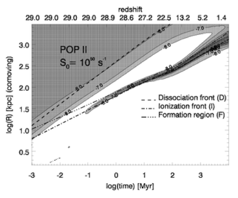
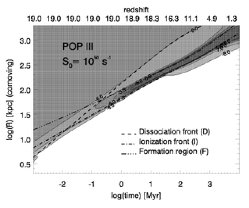
Figure 6: Contours of log$(x_{H_{2}})$ as a function of time and comoving distance from the source. The thick lines show the analytical fits of the photo-dissociation front (D), ionization front (I) and formation region (F). (Top) example of negative feedback: Pop II SED, $S_{0}\simeq 10^{50}$ s^-1, turn-on redshift $z_{i}=29$. The source is at the center of baryonic halo with density profile $n\propto R^{-2}$. (Bottom) example of positive feedback: Pop III SED, $S_{0}\simeq 10^{50}$ s^-1, turn-on redshift $z_{i}=19$.

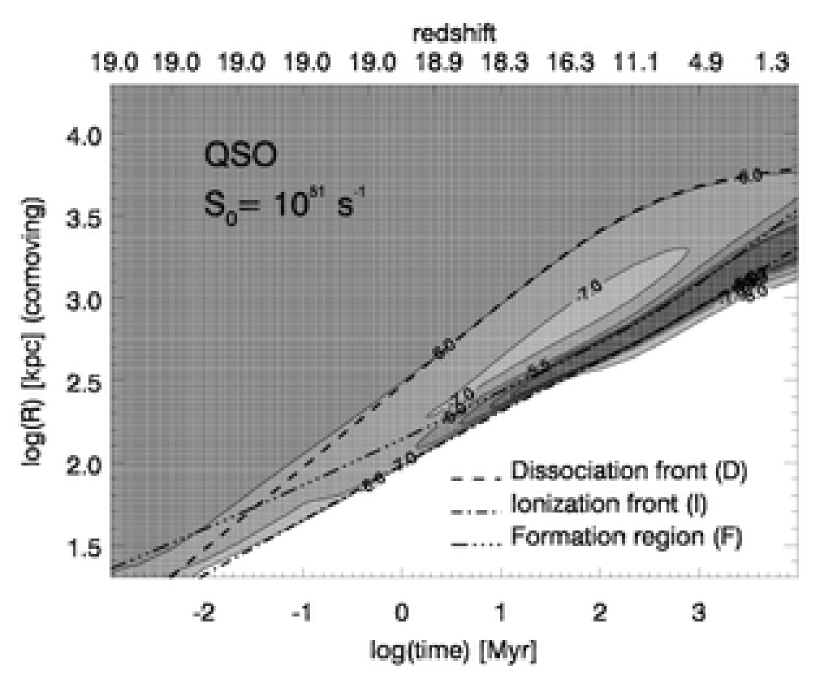
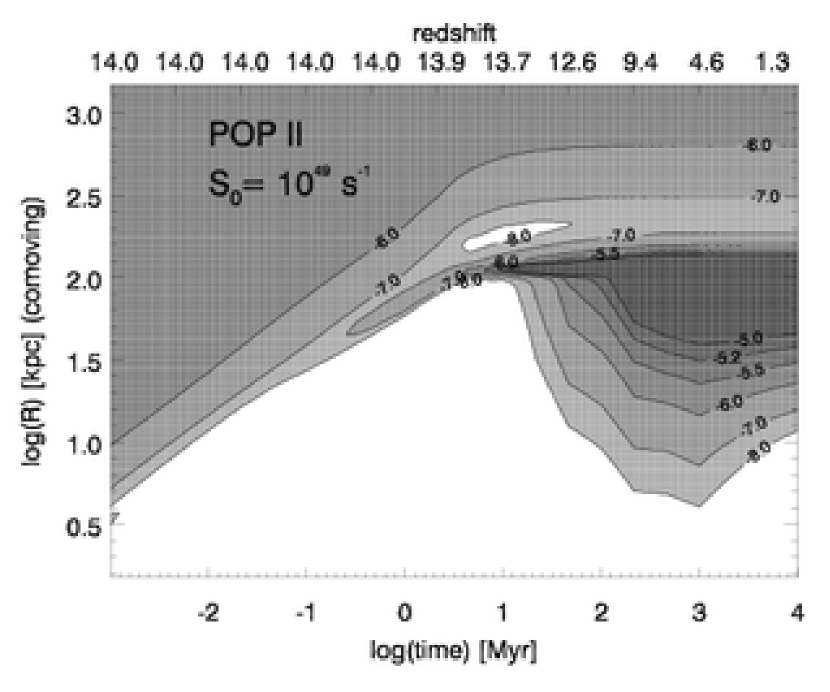
Figure 7: Same as Figure 6. (Top) QSO SED, $S_{0}\simeq 10^{51}$ s^-1, turn-on redshift $z_{i}=19$. (Bottom) fossil H II Region: Pop II SED (instantaneous star formation law), $S_{0}\simeq 10^{49}$ s^-1, turn-on redshift $z_{i}=14$.

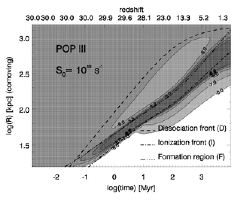
Figure 8: Same as Figure 6. (Top) Pop III SED, $S_{0}\simeq 10^{49}$ s^-1, turn-on redshift $z_{i}=30$. (Bottom) same but including line radiative transfer in H₂ Lyman-Werner bands.

3.2 Analytical Fits

Let us introduce some relevant time scales. The collisional recombination time scales for neutral hydrogen and protons are $t_{HI}=t_{rec}(1-x_{e})/x_{e}^{2}$ and $t_{HII}=t_{rec}/x_{e}$ respectively, where $x_{e}$ is the electron fraction number density. Here we define $t_{rec}=1/(\alpha_{H}^{(2)}n_{H})$ where $\alpha_{H}^{(2)}=2.59\times 10^{-13}$ cm³ s^-1 is the case-B recombination coefficient at $T=10^{4}$ K and $n_{H}(z_{i})=(1.7\times 10^{-7}~{}\text{cm}^{-3})(1+z_{i})^{3}$ is the hydrogen number density for $\Omega_{b}h^{2}=0.019$. The age of the universe $t_{H}$ and $t_{rec}$ at the redshift $z_{i}$ when the source turns on are:

$$t_{H} \approx {2\over 3}{1\over H_{0}\sqrt{\Omega_{0}}}(1+z_{i})^{-3/2}=538\left({1+z_{i}\over 10}\right)^{-3/2}~{}\text{Myr},$$ (8)

$$t_{rec} \approx {1\over\alpha_{H}^{(2)}n_{H}(z_{i})}=720\left({1+z_{i}\over 10}\right)^{-3}~{}\text{Myr}.$$ (9)

If the density of the IGM is constant and uniform, the radius $R_{I}$ of the ionization front is,

$${R_{I}\over R_{S}}=\left[1-\exp\left(-{t\over t_{rec}}\right)\right]^{1\over 3},$$ (10)

where $R_{S}=(3S_{0}t_{rec}/4\pi n_{H}(z_{i})]^{1/3}$ is the Strömgren radius and $t$ is the time the source is on. The typical time for the H II region to reach the Strömgren radius in a non-expanding IGM equals the H⁺ recombination time. A source turning on at redshifts $z_{i}\lesssim 18$, for which $\lambda=t_{H}/t_{rec}\lesssim 2$, produces an H II region that never reaches the Strömgren radius (Donahue & Shull, 1987; Shapiro & Giroux, 1987). In comoving coordinates, it expands forever because of cosmic dilution. This is true only if the source continues to shine with constant photon luminosity $S_{0}$. We therefore remind the reader of another typical time scale, namely the time $t_{burst}\simeq 5-20$ Myr during which an instantaneous burst of star formation produces a substantial amount of ionizing photons.

Based on the simulations, we find analytical relationships that are good fits to the comoving front radii (radius of the ionization sphere, $R_{I}$, radius of the photo-dissociation sphere, $R_{D}$, and outer radius of the PFR, $R_{F}$), the peak H₂ abundance $x_{H_{2},F}$, comoving thickness, $\Delta R_{F}$ and column density, $N_{F}$, of the PFR as a function of time. We also estimate the time scale, $t_{F}$, on which a region in the IGM lies inside the PFR. These relations, without taking into account line radiative transfer, are:

$$R_{D} = (16~{}{\rm kpc})\left({1+z_{i}\over 10}\right)[\beta S_{0,49}f_{2}(t)]^{1\over 2},$$ (11)

$$R_{I} = (21~{}{\rm kpc})[S_{0,49}\langle f_{esc}\rangle f_{1}(t)]^{1\over 3},$$ (12)

$$\Delta R_{I} = (5\times 10^{-5}\gamma~{}{\rm kpc}){(1+z)^{2.3}\over n_{H}(z)}(S_{0,49}\langle f_{esc}\rangle t)^{0.18}$$ (13)

$$= (3.2\gamma~{}{\rm Mpc})\left({1+z_{i}\over 10}\right)^{0.7}{(S_{0,49}\langle f_{esc}\rangle t)^{0.18}\over t_{c}^{0.466}},$$ (14)

$$\Delta R_{F} = {\Delta R_{I}\over 3},$$ (15)

where $S_{0,49}$ is the ionizing photon luminosity in units of $10^{49}$ [photon s^-1 ], $\beta$ and $\gamma$ are fitting parameters (Table 1) that depend on the SED of the object ($\beta=\gamma=1$ for a Pop III SED), and $t$ is the time the source was on in Myr. $\Delta R_{I}$ is the comoving thickness of the ionization front. The functions $f_{1}$ and $f_{2}$ are given by

$$f_{1}(t) = {(8.95\times 10^{5})\lambda\over(1+z_{i})^{3}}\exp{\left({\lambda\over t_{c}}\right)}(t_{c}E_{2}(\lambda/t_{c})-E_{2}(\lambda))~{}\text{Myr},$$ (16)

$$f_{2}(t) = 3t_{H}[1-t_{c}^{-1/3}]~{}\text{Myr},$$ (17)

with $t_{c}=1+t/t_{H}$, $\lambda=t_{H}/t_{rec}$ and $E_{n}(x)$ is the exponential integral of order $n$ (Donahue & Shull, 1987; Shapiro & Giroux, 1987). Note that $f_{1}(t)\sim t$ if $t\ll t_{H}$ and $f_{2}(t)\sim t$ if $\lambda\lesssim 2$ (i.e. $z_{i}\lesssim 18$). Table 1 shows the normalization parameters $\beta,\gamma$ and the ionizing photon luminosity $S_{0,49}$ produced by an instantaneous burst of $\sim 250$ M_⊙ of gas into stars for the SEDs from Pop III, Pop II (continuous star formation) and mini-quasars.

Table 1: Fit parameters for the analytical formulae in § 3.2

Object	$S_{0,49}$	$\beta$	$\gamma$
	(250 M⊙ burst)
Pop II	2.8	2.4	0.67
Pop III	3.2	1.0	1.0
Quasar	–	0.8	1.17

Here the photo-dissociation front is defined as the locus where the molecular abundance is $x_{H_{2}}=10^{-6}$, half the relic H₂ fraction. In the optically thin regime, that is a good approximation in this case, the profile of the H₂ abundance inside the dissociation sphere is exponential: $x_{H_{2}}=2\times 10^{-6}\exp[-\ln(2)R_{D}/r]$. The photo-dissociation front slows down at $t\gtrsim t_{H}$, after the initial $t^{1/2}$ expansion law. At late times the dissociation front approaches the maximum radius $R_{D}=(340\alpha)~{}{\rm kpc}[(1+z_{i})/10]^{1/4}(\beta S_{0,49})^{1/2}$, where $\alpha=[1-(1+z_{i})^{-1/2}]^{1/2}$. The relation $(1+z)=(1+z_{i})t_{c}^{-2/3}$ is used to relate time and redshift. The maximum thickness of the ionization front $\Delta R_{I}=(7\gamma~{}\text{Mpc})[(1+z_{i})/10]^{0.43}(S_{0,49}\langle f_{esc}\rangle)^{0.18}$ is reached at $t=0.6t_{H}$.

When the ionization front is inside the halo with a density profile $n\propto R^{-2}$, where $R$ is the radius, we find $\log R_{I}\propto(\log t)^{2}$. The emerging spectrum in this case is harder. The photo-dissociation front, if we do not take into account self-shielding in H₂ lines, is independent of the chosen density profile of the gas. The width of the PFR inside the halo is smaller by a factor $n^{-1}$, but its column density increases as $n$.

We have made some numerical “experiments” to test which species have abundances equal to their equilibrium values. Only H^- can be safely considered in equilibrium. Nevertheless, for H₂ the equilibrium abundance is not a good approximation, it is an helpful estimate since can be derived analytically (Donahue & Shull, 1991; Abel et al., 1997) and will give us the functional form for the fitting formula. If we consider only the formation process through H^-, with rate $k_{f}(T)x_{H^{-}}$ and photo-dissociation by photons with $h\nu>0.755$ eV, the equilibrium H₂ abundance in the PFR is $x_{{H_{2}},F}\propto n_{H}(z)k_{f}(T)x_{H^{-}}F_{s}^{-1}\propto(1+z)R_{I}^{2}/(\beta S_{0,49})$, where $F_{s}\propto\beta S_{0,49}(1+z)^{2}R_{I}^{-2}$ is the dissociating flux. In all the simulations, after the PFR shell starts to build up, the abundance of H^- reaches an equilibrium value $x_{H^{-}}\simeq 5\times 10^{-7}$. The best fit differs slightly from the expression above because of a redshift dependence of the formation rates:

$$x_{{H_{2}},F} = (1.74\times 10^{-9}){(1+z)^{1.3}\over\beta S_{0,49}}R_{I}^{2}$$ (18)

$$= 1.6\times 10^{-5}\left({1+z_{i}\over 10}\right)^{1.3}\beta^{-1}S_{0,49}^{-1/3}\langle f_{esc}\rangle^{2/3}{t^{2/3}\over t_{c}^{0.87}}.$$ (19)

The maximum value of $x_{{H_{2}},F}$, reached at $t=(10/3)t_{H}$, is given by

$$x_{{H_{2}},F}^{max}=5.9\times 10^{-4}\left({1+z_{i}\over 10}\right)^{1/3}S_{0,49}^{-1/3}\langle f_{esc}\rangle^{2\over 3}.$$ (20)

From equations (11-19) it is easy to derive useful relationships to quantify the importance of positive feedback as a function of the unknown free parameters. We will use these relationships in the next section. The ratio

$${R_{D}\over R_{I}}=0.76\left({1+z_{i}\over 10}\right)\langle f_{esc}\rangle^{-1/3}\beta^{1/2}S_{0,49}^{1/6}\,g(t)$$ (21)

reaches the maximum value of

$$\left({R_{D}\over R_{I}}\right)^{max}=1.6\left({1+z_{i}\over 10}\right)^{3/4}\langle f_{esc}\rangle^{-1/3}\beta^{1/2}S_{0,49}^{1/6}$$ (22)

at $t\simeq 0.9t_{H}$ where the function $g(t)=[f_{1}(t)]^{1/2}[f_{2}(t)]^{-1/3}$ scales as $g(t)\simeq t^{1/6}$ if $t<t_{H}$ and $\lambda<1$. The function has a maximum value of $g=0.75t_{H}^{1/6}=2.1[(1+z_{i})/10]^{-1/4}$ at $t=0.9t_{H}$.

It is also useful to estimate the H₂ column density, $N_{F}$, of the PFR, and the time scale, $t_{F}$, on which a region in the IGM can be engulfed by the PFR:

$$N_{F}\simeq{nx_{{H_{2}},F}\Delta R_{F}\over 1+z}=(1.6\times 10^{13}~{}\text{cm}^{-2}){\gamma\over\beta}\left({1+z_{i}\over 10}\right)^{2.6}{(\langle f_{esc}\rangle t)^{0.85}\over S_{0,49}^{0.15}~{}t_{c}^{1.7}}$$ (23)

with the maximum value of

$$N_{F}^{max}=(9\times 10^{14}~{}\text{cm}^{-2}){\gamma\over\beta}\left({1+z_{i}\over 10}\right)^{1.3}{\langle f_{esc}\rangle^{0.85}\over S_{0,49}^{0.15}}$$ (24)

at $t\simeq 0.9t_{H}$, and

$$t_{F}=\Delta R_{F}\left({dR_{I}\over dt}\right)^{-1}=(152t\gamma)\left({1+z_{i}\over 10}\right)^{0.7}{(S_{0,49}\langle f_{esc}\rangle t)^{-0.15}\over t_{c}^{0.47}}.$$ (25)

Finally, we derive the ratio $R_{D}/R_{F}=R_{D}/(R_{I}+\Delta R_{F})=(R_{D}/R_{I})(1+\Delta R_{F}/R_{I})^{-1}$ that gives us an idea of the fraction of the IGM volume in which the molecular hydrogen is destroyed:

$${R_{D}\over R_{F}}={R_{D}\over R_{I}}\left[1+51\gamma\left({1+z\over 10}\right)^{0.7}(S_{0,49}\langle f_{esc}\rangle t)^{-0.15}\right]^{-1}$$ (26)

with the maximum value of

$$\left({R_{D}\over R_{F}}\right)^{max}={0.15\beta^{1/2}\over\gamma}\left[\langle f_{esc}\rangle\left({1+z_{i}\over 10}\right)\right]^{-0.18}S_{0,49}^{1/3}$$ (27)

at $t\simeq 0.9t_{H}$.

4 Discussion: Negative or Positive Feedback ?

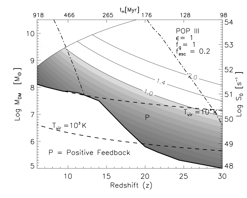
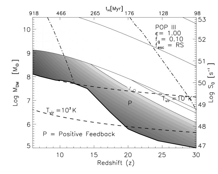
Figure 9: The contours show $R_{D}/R_{F}$ for our standard model and cosmological parameters (§ 1). The shaded region ($R_{D}/R_{F}<1$) shows the redshift and halo masses where positive feedback is dominant. The thick solid line shows the minimum mass needed to collapse according to Abel et al. (1998). Parameters: $\langle f_{esc}\rangle$ = escape fraction, $\epsilon=$ star formation efficiency normalized to the Milky-Way, $f_{g}=$ collapsed gas fraction, $S_{0}=(1.14\times 10^{49}{\rm s}^{-1})\epsilon f_{g}(M_{DM}/10^{6}$ M${}_{\odot})$. The dot-dashed lines show the collapse redshift of $1\sigma$ and $3\sigma$ perturbations according to linear theory. (Top) Pop III SED, $\epsilon=1$, $f_{g}=1$ and $\langle f_{esc}\rangle$ $=0.2$. (Bottom) Pop III SED, $\epsilon=1$, $f_{g}=0.1$ and $\langle f_{esc}\rangle$ given by the analytical formula derived in Ricotti & Shull (2000).

In this section, we use the analytical relationships found in § 3.2 to quantify the importance of the positive feedback as a function of the free parameters of the model. The free parameters are: the Lyc escape fraction, $\langle f_{esc}\rangle$, the star formation efficiency $\epsilon$ normalized to that in the Milky Way, and the collapsed gas fraction, $f_{g}$. For a fixed cosmology, the ionizing photon luminosity is $S_{0}=(1.14\times 10^{49}~{}\text{s}^{-1})\epsilon f_{g}(M_{DM}/10^{6}$ M${}_{\odot})$ [see Ricotti & Shull (2000) for details]. We quantify the importance of the positive feedback by showing in Figure 9 isocontours of constant ratio, $R_{D}/R_{F}$, of the photo-dissociation front radius to the formation front radius 10 Myr after the source turned on. Here the radius of the dissociation front $R_{D}$ is defined as the locus where the relic molecular abundance has dropped to $x_{H_{2}}=10^{-8}$, therefore it is smaller by a factor $\ln(200)/\ln(2)\sim 7.6$ with respect to the values given in the previous paragraph. Clearly, if $R_{D}/R_{F}<1$ the dissociation region does not exist. Instead, the H₂ abundance could increase with respect to the relic value $x_{H_{2}}\approx 2\times 10^{-6}$ (as an example see Figure 6 [bottom]). Therefore, $R_{D}/R_{F}$ gives us an idea of the mean molecular abundance in the IGM and the opacity of the IGM to the photo-dissociating background.

We find that the existence of positive feedback depends crucially on $\langle f_{esc}\rangle$ and the SED of the first objects (Pop III, Pop II or AGN). Figure 9 shows the parameter space where positive feedback is possible in the particular case of a Pop III SED. The contour lines show $R_{D}/R_{F}$ as a function of redshift and mass of the halo. The shaded region shows the parameter space where $R_{D}/R_{F}<1$, in which case the PFR fills up the region between the H II region and the photo-dissociation front. At small redshifts, the boundary of the shaded region is produced by the additional constraint that the H₂ abundance of the PFR has to be $x_{H_{2}}>10^{-5}$. The choice of this value is somewhat arbitrary, but the main purpose is to show the H₂ abundance in the PDF as a function of the redshift and halo mass. The thick solid line at the bottom is the minimum mass to collapse as a function of redshift according to the criteria of Abel et al. (1998). The two dashed lines show objects with virial temperatures of $T_{vir}=10^{3}$ K and $T_{vir}=10^{4}$ K; protogalaxies that lie above $T_{vir}=10^{4}$ K are not subject to negative/positive feedback because they can cool by H I line excitation (Ly$\alpha$). The minimum mass for collapse is calculated assuming that the object lies outside of a photo-dissociation region or a PFR and that the dissociating background is negligible. The amount of H₂ formed in a just-virialized object does not depend on the initial H₂ abundance, but it is sensitive to the electron fraction. For this reason, protogalaxies less massive than those found in the Abel et al. (1998) calculations can form inside a PFR. Finally, we note that the presence of PFRs will increase the opacity of the IGM in the Lyman-Werner lines, further decreasing the intensity of the dissociating UV background. All these effects have to be included in a 3D cosmological simulation with radiative transfer in order to understand their global effect on structure formation and the star formation history.

5 IGM optical depth in the Lyman-Werner bands

In this section we estimate the IGM optical depth in the Lyman-Werner bands that arises from the absorption in 76 narrow H₂ lines from $J=0,1$ in $v=0$ at different redshift. This calculation is analogous to the one in Haiman et al. (2000). We repeat it because we disagree with their technical analysis of H₂ line scattering and fluorescence. Haiman et al. (2000) assumed that only the fraction of absorptions that decay to the dissociating continuum remove photons from the UVB (about 11% of the time). For the other 89% of the absorptions, they assume that the Lyman-Werner photon is re-emitted at the same frequency, with no net effect. This is not correct. Following the absorption in the Lyman or Werner bands, the molecule decays to a variety of ro-vibrational levels in the ground electronic state because the quadrupole transitions within the electronic excited state are much slower. The H₂ either decays to the $b^{3}\Sigma^{+}_{u}$ (anti-bonding) state which decays to the vibrational continuum (pre-dissociation) or to a bound vibrational-rotational level in the electronic ground state ($X^{1}\Sigma_{g}^{+}$). At moderate UV intensities, the subsequent infrared cascade through the bound levels of the ground electronic state is entirely determined by the radiative decay rates (Black & Dalgarno, 1976). From the cascade probabilities, Shull (1978) computed that a Lyman-Werner photon has a 14% probability, on average, to be re-emitted at the same frequency. Approximately 12% of the absorption transitions dissociate and 74% fluoresce to excited $(v,J)$ levels of $X^{1}\Sigma_{g}^{+}$. Roughly speaking, the probability to decay to one of the other 14 bound vibrational levels is about 6%. Therefore, only 14% of the time the Lyman-Werner photon is resonantly scattered following an absorption. The other 86% of the time, H₂ dissociates or the photon is split into infrared and less energetic (about 1 eV energy loss) UV photons that are removed from the Lyman-Werner bands right away or after a few absorptions.

Therefore, the H₂ optical depth of the IGM is given by

$$\tau_{\nu}(z_{ob},z_{em})={\pi e^{2}\over m_{e}c}\sum_{i=n_{1}(\nu)}^{n_{2}(\nu)}f_{osc,i}(1-f_{i,\nu^{\prime\prime}=0})\int_{z_{ob}}^{z_{em}}dz^{\prime}~{}c{dt\over dz^{\prime}}~{}n_{H}(z^{\prime})x_{H_{2}}(z^{\prime})\phi(\nu^{\prime},\nu_{i})$$ (28)

where $z_{ob}$ and $z_{em}$ are the observer and emission redshifts, $\nu^{\prime}=\nu(1+z_{em})/(1+z_{ob})$, $n_{H}(z)=(1.12\times 10^{-5}~{}\text{cm}^{-3})\Omega_{b}h^{2}(1-Y_{P})(1+z)^{3}$ is the neutral H number density in the IGM, $\phi$ is the line profile, $f_{osc,i}$ is the oscillator strength, and $f_{i,\nu^{\prime\prime}=0}$ the probability to decay to the ground vibrational level of the $X^{1}\Sigma_{g}^{+}$ state for the $i^{th}$ line calculated from Black & Dalgarno (1976). The maximum redshift interval a UV photon can travel before it is absorbed by a neutral atom corresponds to the redshift between two H I resonances in the higher Lyman series, the “dark screen” approximation of Haiman et al. (2000). Therefore a photon is subject to the absorption from a subset of the 76 Lyman-Werner lines, $n_{1}(\nu)\leq i\leq n_{2}(\nu)$, where $n_{1}(\nu)$ is the first Lyman-Werner line with frequency just above $\nu$, and $n_{2}(\nu)>n_{1}(\nu)$ is the Lyman-Werner line with frequency just below the next higher H I Lyman line with frequency $>\nu$.

It is possible to write an approximate analytical solution of equation (28), if we assume Gaussian line profiles, $\phi_{G}(\nu,\nu_{i})=(1/\sqrt{\pi}\Delta\nu_{i})\exp[-(\nu-\nu_{i})^{2}/\Delta\nu_{i}^{2}]$, where $\Delta\nu_{i}=3\times 10^{-7}\nu_{i}T_{IGM}^{1/2}$ is the Doppler width of the H₂ line $i$, or Lorentzian line profiles $\phi_{L}(\nu,\nu_{i})=(\Gamma_{i}/2\pi)/[(\nu-\nu_{i})^{2}+(\Gamma_{i}/2)^{2}]$, where $\Gamma_{i}=\gamma_{i}/2\pi$ and $\gamma_{i}=\sum_{l}A(i\rightarrow l)$ is the natural width of the $i^{th}$ H I line. For a constant $x_{H_{2}}=2\times 10^{-6}$ molecular abundance, we have

$$\tau_{\nu}(z_{ob},z_{em})\simeq 3.28\times 10^{15}\left({1+z_{ob}\over\nu}\right)^{3/2}\sum_{i=n_{1}(\nu)}^{n_{2}(\nu)}f_{osc,i}(1-f_{i,\nu^{\prime\prime}=0})\nu_{i}^{1/2}\Phi(\nu^{\prime})$$ (29)

where,

$$\Phi(\nu^{\prime})=\begin{cases}{1\over 2}\left[\text{erf}\left({\nu^{\prime}-\nu_{i}\over\Delta\nu_{i}}\right)-\text{erf}\left({\nu-\nu_{i}\over\Delta\nu_{i}}\right)\right],&\text{for Gaussian profile}\\ \\ {1\over\pi}\left[\arctan\left({\nu^{\prime}-\nu_{i}\over\Gamma_{i}}\right)-\arctan\left({\nu-\nu_{i}\over\Gamma_{i}}\right)\right],&\text{for Lorenzian profile}\end{cases}$$ (30)

and $\text{erf}(x)$ is the error function. In Figure 10, we show the H₂ total optical depth (i.e., up to the maximum $z_{em}$ visible to the observer) of the IGM in the Lyman-Werner bands at redshifts $z=30$ (solid line) and $z=15$ (dashed line). The opacity at energies less than Ly$\beta$ ($h\nu<12.09$ eV) is produced by the H₂ Lyman lines. At energies higher than Ly$\beta$, the H₂ Werner lines are also important. The maximum opacity that we find is $\tau\sim 2$, about 6 times higher than that found by Haiman et al. (2000). The background flux is thus reduced by an order of magnitude if we assume an average molecular fraction $x_{H_{2}}=2\times 10^{-6}$.

Figure 10: Total H₂ optical depth of the IGM in the Lyman-Werner bands. The solid line is for an observer at redshift $z_{ob}=30$ and the dashed line at $z_{ob}=15$. We assume a constant $x_{H_{2}}=2\times 10^{-6}$.

Figure 11: In the plot we show the function [$\text{erf}(x^{\prime})-\text{erf}(x)$], where $x^{\prime}=(\nu^{\prime}-\nu_{i})/\Delta\nu_{i}$ and $x=(\nu-\nu_{i})/\Delta\nu_{i}$. According to equation (29), this function is proportional to the optical depth of an H₂ line through a gas of constant density and molecular fraction. When the source redshift $z_{em}$ increases with respect to the observer redshift $z_{ob}$, the profile becomes wider, and the optical depth tends toward the asymptotic value $\tau_{max}$ in equation (31). The profiles are shown at $\log[(z_{em}-z_{ob})/(1+z_{ob})]=-3.5,-4,-4.5,...,-7$. The gas temperature is either $T=10^{4}$ K (solid lines) and $T=10$ K (dashed lines).

Figure 12: Total optical depth, $\langle\tau_{IGM}\rangle$, for photo-dissociation of H₂ in the IGM as a function of the comoving distance from a source at $z_{em}=30$. $\langle\tau_{IGM}\rangle$ includes the opacity of H₂ and H I lines and is weighted on the photo-dissociation rate; see equation (33). The solid line is calculated assuming a Voigt profile for the Lyman series hydrogen lines, therefore including the effect of the damping wings. The dashed line is calculated neglecting H I damping wings. The insert is a zoom of the inner few Mpc, and the arrow indicates the distance at which the absorption lines are redshifted about one line width for a gas at $T=10^{4}$ K.

For the Gaussian line profile, the expression inside the square brackets of equation (30) tends to the asymptotic value of 2 when $(1+z_{em})/(1+z_{ob})>\Delta\nu_{i}$. The maximum optical depth of the $i^{th}$ line is therefore

$$\tau_{max}(z_{ob})\simeq x_{H_{2}}n_{H}(z=0){c\over H_{0}}\sigma f_{osc,i}{(1+z_{ob})^{3/2}\over\nu_{i}}\simeq 0.1\left({x_{H_{2}}\over 2\times 10^{-6}}\right)\left({12~{}{\rm eV}\over h\nu_{i}}\right)\left({f_{osc,i}\over 10^{-2}}\right)\left({1+z_{ob}\over 30}\right)^{3/2}.$$ (31)

In Figure 11, we show the optical depth through a constant density and molecular fraction gas for a single line. When the source redshift $z_{em}$ increases, the profile becomes wider and the optical depth tends to the asymptotic value $\tau_{max}$ in equation (31).

Finally, we calculate the total optical depth of the IGM as a function of distance from a single source. We also include in the calculation the Lyman series lines of H I and we investigate the importance of the damping-wings of the heavily saturated lines. The mean optical depth for photo-dissociation, $\langle\tau_{IGM}\rangle$, can be calculated by solving the following equations:

$$k_{diss} = \text{const}\sum_{i=1}^{76}f_{osc,i}f_{diss}\int_{\nu}d\nu^{\prime}{J_{\nu^{\prime}}\over h\nu^{\prime}}~{}\phi(\nu^{\prime},\nu_{i}),$$ (32)

$$k_{diss}\exp{(-\langle\tau_{IGM}\rangle)} = \text{const}\sum_{i=1}^{76}f_{osc,i}f_{diss}\int_{\nu}d\nu^{\prime}{J_{\nu^{\prime}}\over h\nu^{\prime}}~{}\phi(\nu^{\prime},\nu_{i})e^{-\tau_{IGM}(\nu^{\prime},z_{em},z_{ob})}$$ (33)

where $k_{diss}$ is the photo-dissociation rate and where const=$4\pi x_{H_{2}}n_{H}(z_{ob})\sigma$ with $\sigma=(\pi e^{2}/m_{e}c)$. Note that $\tau_{IGM}$ differs from $\tau_{\nu}$ in equation (29) since it includes the opacity of both H₂ and H I lines. In Figure 12 we show $\langle\tau_{IGM}\rangle$ as a function of the comoving distance (and $z_{ob}<z_{em}$) from a source at $z_{em}=30$. The solid line is calculated assuming a Voigt profile for the Lyman series hydrogen lines, therefore including the effect of line saturation. The dashed line is calculated neglecting line saturation. The insert is a zoom of the inner few Mpc, and the arrow indicates the distance at which the absorption lines are redshifted about one line width for gas at $T=10^{4}$ K. Both Figure 12 and Figure 5 show clearly that the opacity at comoving distances from the source of less than 1 Mpc is produced in the PFR shell. The IGM opacity starts to be important around 10 Mpc. This reduces the photo-dissociation radius of the strongest sources at high redshift.

We remind the reader that all the calculations in this section assume a constant molecular fraction in the IGM of $x_{H_{2}}=2\times 10^{-6}$. In order to calculate a realistic average molecular fraction in the IGM as a function of the redshift, we need to calculate the filling factor of the photo-dissociation regions, PFR and the H₂ formed inside relic H II regions. Only with a 3D radiative transfer simulation will it be possible to treat self-consistently the aforementioned feedback effects.

6 Discussion and Summary

The results of this work reinforce the possibility that the population of small mass primordial galaxies (Pop III) could exist, without being immediately suppressed by radiative feedback. A quantitative answer to this question has to be given by high-resolution cosmological simulations. Until the build-up of the dissociating background, local feedback effects regulate star formation. When the star formation is suppressed in a halo, it is reasonable to expect that H II regions start to recombine. The relic H II region, as shown in § 3, produces new molecular hydrogen and perhaps a second burst of star formation. This is especially effective at high redshifts where the density of the IGM and protogalaxies is higher and the physical scales are smaller. Thus, at these redshifts, it is easier to believe that star formation is bursting rather than continuous. The picture that could emerge from numerical simulations is that H II regions and photo-dissociation regions in the IGM are short-lived instead of continuously expanding, as in the reionization simulations of Gnedin (2000). This will have important effects on the distribution of the metals and the chemical evolution of galaxies.

In summary, our key results are:

(1) We have found a new positive feedback effect on the formation of H₂. Each source of radiation produces a shell (PFR: positive feedback region) of H₂ in front of the H II region with a thickness of several kpc and peak abundance $x_{H_{2}}\sim 10^{-4}$. The H₂ column density of the PFR is typically $N_{F}(H_{2})\sim 10^{14}-10^{15}$ cm^-2. Fossil H II regions, if they exist, are an important mechanism of H₂ production, both in the IGM and inside protogalaxies.

(2) The PFR can be optically thick in the lines of the H₂ Lyman-Werner bands. The implication is twofold: (i) the photo-dissociation region around each single source is about 1.5 times smaller than in the optically thin case; (ii) the H₂ optical depth of the IGM increases. In a later paper, we will calculate the IGM optical depth and the effect on the intensity of the photo-dissociating background by means of cosmological simulations.

(3) We provide analytical formulae that fit the simulation results, in order to make a parametric study of the importance of positive feedback as a function of redshift. The most important parameters are $\langle f_{esc}\rangle$ and the SED of the sources (Pop III, Pop II or AGN). If $\langle f_{esc}\rangle$ is not extremely small, PFRs have important effects on the opacity of the IGM to the H₂ photo-dissociating background and the size of photo-dissociation regions.

(4) The background opacity of the IGM in the H₂ Lyman-Werner bands is about unity if $x_{H_{2}}=2\times 10^{-6}$. Therefore, if the relic molecular hydrogen is not immediately destroyed, it can decrease the photo-dissociating background flux by about an order of magnitude.

The aforementioned results are the foundations on which we will construct a cosmological simulation in which these effects are treated self-consistently.

References

- Abel et al. (1998) Abel, T., Anninos, P., Norman, M. L., & Zhang, Y. 1998, ApJ, 508, 518
- Abel et al. (1997) Abel, T., Anninos, P., Zhang, Y., & Norman, M. L. 1997, New Astronomy, 2, 181
- Abel et al. (2000) Abel, T., Bryan, G. L., & Norman, M. L. 2000, ApJ, 540, 39
- Black & Dalgarno (1976) Black, J. H., & Dalgarno, A. 1976, ApJ, 203, 132
- Bromm et al. (1999) Bromm, V., Coppi, P. S., & Larson, R. B. 1999, ApJ, 527, L5
- Burles & Tytler (1998) Burles, S., & Tytler, D. 1998, ApJ, 499, 699
- Ciardi et al. (2000) Ciardi, B., Ferrara, A., & Abel, T. 2000, ApJ, 533, 594
- Ciardi et al. (2000) Ciardi, B., Ferrara, A., Governato, F., & Jenkins, A. 2000, MNRAS, 314, 611
- Croft et al. (1999) Croft, R. A. C., Weinberg, D. H., Pettini, M., Hernquist, L., & Katz, N. 1999, ApJ, 520, 1
- de Bernardis et al. (2000) de Bernardis, P., et al. 2000, Nature, 404, 955
- Donahue & Shull (1987) Donahue, M., & Shull, J. M. 1987, ApJ, 323, L13
- Donahue & Shull (1991) Donahue, M., & Shull, J. M. 1991, ApJ, 383, 511
- Dove et al. (2000) Dove, J. B., Shull, J. M., & Ferrara, A. 2000, ApJ, 531, 846
- Ferrara (1998) Ferrara, A. 1998, ApJ, 499, L17
- Fuller & Couchman (2000) Fuller, T. M., & Couchman, H. M. P. 2000, ApJ, 544, 6
- Galli & Palla (1998) Galli, D., & Palla, F. 1998, A&A, 335, 403
- Garnavich et al. (1998) Garnavich, P. M., et al. 1998, ApJ, 509, 74
- Glover & Brand (2001) Glover, S. C. O., & Brand, P. W. J. L. 2001, MNRAS, 321, 385
- Gnedin (2000) Gnedin, N. Y. 2000, ApJ, 535, 530
- Gnedin & Gnedin (1998) Gnedin, N. Y., & Gnedin, O. Y. 1998, ApJ, 509, 11
- Haiman et al. (2000) Haiman, Z., Abel, T., & Rees, M. J. 2000, ApJ, 534, 11
- Haiman & Loeb (1997) Haiman, Z., & Loeb, A. 1997, ApJ, 483, 21
- Haiman et al. (1996) Haiman, Z., Rees, M. J., & Loeb, A. 1996, ApJ, 467, 522
- Hamilton & Tegmark (2000) Hamilton, A. J. S., & Tegmark, M. 2000, submitted to MNRAS (astro-ph/0008392)
- Hollenbach & McKee (1979) Hollenbach, D., & McKee, C. F. 1979, ApJS, 41, 555
- Hui & Gnedin (1997) Hui, L., & Gnedin, N. Y. 1997, MNRAS, 292, 27
- Lange et al. (2001) Lange, A., et al. 2001, Phys. Rev. D, 63, 042001
- Leitherer et al. (1995) Leitherer, C., Ferguson, H. C., Heckman, T. M., & Lowenthal, J. D. 1995, ApJ, 454, L19
- Lepp & Shull (1984) Lepp, S., & Shull, J. M. 1984, ApJ, 280, 465
- Machacek et al. (2001) Machacek, M. E., Bryan, G. L., & Abel, T. 2001, ApJ, 548, 509
- Martin et al. (1996) Martin, P. G., Schwarz, D. H., & Mandy, M. E. 1996, ApJ, 461, 265
- McCray & Kafatos (1987) McCray, R., & Kafatos, M. 1987, ApJ, 317, 190
- McDonald et al. (2000) McDonald, P., Miralda-Escudé, J., Rauch, M., Sargent, W. L. W., Barlow, T. A., Cen, R., & Ostriker, J. P. 2000, ApJ, 543, 1
- Nakamura & Umemura (1999) Nakamura, F., & Umemura, M. 1999, ApJ, 515, 239
- Navarro et al. (1997) Navarro, J. F., Frenk, C. S., & White, S. D. M. 1997, ApJ, 490, 493
- Oh (2001) Oh, S. P. 2001, ApJ, 553, 499
- Omukai & Nishi (1998) Omukai, K., & Nishi, R. 1998, ApJ, 508, 141
- Omukai & Nishi (1999) Omukai, K., & Nishi, R. 1999, ApJ, 518, 64
- Perlmutter et al. (1998) Perlmutter, S., et al. 1998, Nature, 391, 51
- Ricotti et al. (2001) Ricotti, M., Gnedin, N. Y., & Shull, J. M. 2001, in ASP Conf. Ser. 222: The Physics of Galaxy Formation
- Ricotti & Shull (2000) Ricotti, M., & Shull, J. M. 2000, ApJ, 542, 548
- Riess et al. (1998) Riess, A. G., et al. 1998, AJ, 116, 1009
- Shapiro & Giroux (1987) Shapiro, P. R., & Giroux, M. L. 1987, ApJ, 321, L107
- Shapiro & Kang (1987) Shapiro, P. R., & Kang, H. 1987, ApJ, 318, 32
- Shull (1978) Shull, J. M. 1978, ApJ, 219, 877
- Stecher & Williams (1967) Stecher, T. P., & Williams, D. A. 1967, ApJ, 149, L29
- Tegmark et al. (1997) Tegmark, M., Silk, J., Rees, M. J., Blanchard, A., Abel, T., & Palla, F. 1997, ApJ, 474, 1
- Tegmark et al. (2000) Tegmark, M., Zaldarriaga, M., & Hamilton, A. J. S. 2000, submitted (astro-ph/0008167)
- Tumlinson & Shull (2000) Tumlinson, J., & Shull, J. M. 2000, ApJ, 528, L65
- Venkatesan et al. (2001) Venkatesan, A., Giroux, M. L., & Shull, J. M. 2001, submitted