*

Abstract

We present here a new algorithm for the fast computation of $N$–point correlation functions in large astronomical data sets. The algorithm is based on kd-trees which are decorated with cached sufficient statistics thus allowing for orders of magnitude speed–ups over the naive non-tree-based implementation of correlation functions. We further discuss the use of controlled approximations within the computation which allows for further acceleration. In summary, our algorithm now makes it possible to compute exact, all–pairs, measurements of the 2, 3 and 4–point correlation functions for cosmological data sets like the Sloan Digital Sky Survey (SDSS; York et al. 2000) and the next generation of Cosmic Microwave Background experiments (see Szapudi et al. 2000).

1 Introduction

Correlation functions are some of the most widely used statistics within astrophysics (see Peebles 1980 for a extensive review). They are often used to quantify the clustering of objects in the universe (e.g. galaxies, quasars etc.) compared to a pure Poission process. More recently, they have also been used to measure fluctuations in the Cosmic Microwave Background (see Szapudi et al. 2000). On large scales, the higher–order correlation functions (3-point and above) can be used to test several fundamental assumptions about the universe; for example, our hierarchical scenario for structure formation, the Gaussianity of the initial conditions as well as testing various models for the biasing between the luminous and dark matter. The reader is referred to Szapudi (2000), Szapudi et al. (1999a,b) and Scoccimarro (2000; and references therein) for an overview of the usefulness of $N$–point correlation functions in constraining cosmological models.

Over the coming decade, several new, massive cosmological surveys will become available to the astronomical community. In this new era, the quality and quantity of data will warrant a more sophisticated analysis of the higher–order correlation functions of galaxies (and other objects) over the largest range of scales possible. Our ability to perform such studies will be severely limited by the computational time needed to compute such functions and no-longer by the amount of data available. In this paper, we address this computational “bottle-neck” by outlining a new algorithm that uses innovative computer science to accelerate the computation of $N$–point correlation functions far beyond the naive $O(R^{N})$ scaling law (where $R$ is the number of objects in the dataset and $N$ is the power of correlation function desired).

The algorithm presented here was developed as part of the “Computational AstroStatistics” collaboration (see Nichol et al. 2000) and is a member of a family of algorithms for a very general class of statistical computations, including nearest-neighbor methods, kernel density estimation, and clustering. The work presented here was initially presented by Gray & Moore (2001) and will soon be discussed in a more substantial paper by Connolly et al. (2001). In this conference proceeding, we provide a brief review of kd-trees (Section 2), a discussion of the use of kd-trees in range searches (Section 3), an overview of the development of a fast $N$–point correlation function code (Section 4) as well as presenting the concept of controlled approximations in the calculation of the correlation function (Section 5). In Section 6, we provide preliminary results on the computation speed-up achieved with this algorithm and discuss future prospects for further advances in this field through the use of other tree structures.

2 Review of kd-trees

Our fast $N$–point correlation function algorithm is built upon the kd-tree data structure which was introduced by Friedman et al. (1977). A kd-tree is a way of organizing a set of datapoints in $k$-dimensional space in such a way that once built, whenever a query arrives requesting a list all points in a neighborhood, the query can be answered quickly without needing to scan every single point.

The root node of the kd-tree owns all the data points. Each non-leaf-node has two children, defined by a splitting dimension ${n}.{\mbox{\scriptsize\sc SplitDim}}$ and a splitting value ${n}.{\mbox{\scriptsize\sc SplitValue}}$. The two children divide their parent’s data points between them, with the left child owning those data points that are strictly less than the splitting value in the splitting dimension, and the right child owning the remainder of the parent’s data points:

$${\mbox{\bf x}}_{i}\in{n}.{\mbox{\scriptsize\sc Left}} \Leftrightarrow {\mbox{\bf x}}_{i}[{n}.{\mbox{\scriptsize\sc SplitDim}}]<{n}.{\mbox{\scriptsize\sc SplitValue}}\mbox{ and }{\mbox{\bf x}}_{i}\in n$$ (1)

$${\mbox{\bf x}}_{i}\in{n}.{\mbox{\scriptsize\sc Right}} \Leftrightarrow {\mbox{\bf x}}_{i}[{n}.{\mbox{\scriptsize\sc SplitDim}}]\geq{n}.{\mbox{\scriptsize\sc SplitValue}}\mbox{ and }{\mbox{\bf x}}_{i}\in n$$ (2)

As an example, some of the nodes of a kd-tree are illustrated in Figures 1.

kd-trees are usually constructed top-down, beginning with the full set of points and then splitting in the center of the widest dimension. This produces two child nodes, each with a distinct set of points. This procedure is then repeated recursively on each of the two child nodes.

A node is declared to be a leaf, and is left unsplit, if the widest dimension of its bounding box is $\leq$ some threshold, MinBoxWidth. A node is also left unsplit if it denotes fewer than some threshold number of points, $r_{\mbox{\scriptsize min}}$. A leaf node has no children, but instead contains a list of $k$-dimensional vectors: the actual datapoints contained in that leaf. The values $\mbox{\sc MinBoxWidth}=0$ and $r_{\mbox{\scriptsize min}}=1$ would cause the largest kd-tree structure because all leaf nodes would denote singleton or coincident points. In practice, we set MinBoxWidth to $1\%$ of the range of the data point components and $r_{\mbox{\scriptsize min}}$ to around 10. The tree size and construction thus cost considerably less than these bounds because in dense regions, tiny leaf nodes are able to summarize dozens of data points. The operations needed in tree-building are computationally trivial and therefore, the overhead in constructing the tree is negligible. Also, once a tree is built it can be re-used for many different analysis operations.

Since the introduction of kd-trees, many variations of them have been proposed and used with great success in areas such as databases and computational geometry (Preparata & Shamos 1985). R-trees (Guttman 1984) are designed for disk resident data sets and efficient incremental addition of data. Metric trees (see Uhlmann 1991) place hyperspheres around tree nodes, instead of axis-aligned splitting planes. In all cases, the algorithms we discuss in this paper could be applied equally effectively with these other structures. For example, Moore (2000) shows the use of metric trees for accelerating several clustering and pairwise comparision algorithms.

3 Range Searching

Before proceeding to fast $N$–point calculations, we will begin with a very standard kd-tree search algorithm that could be used as a building block for fast 2-point computations.

For simplicity of exposition we will assume the every node of the kd-tree contains one extra piece of information: the bounding box of all the points it contains. Call this box ${n}.{\mbox{\scriptsize\sc BoundBox}}$. The implication of this is that every node must contain two new $k$ dimensional vectors to represent the lower and upper limits of each dimension of the bounding box. The range search operation takes two inputs. The first is a $k$-dimensional vector q called the query point. The second is a separation distance ${\mbox{\it s}}_{hi}$. The operation returns the complete set of points in the kd-tree that lie within distance ${\mbox{\it s}}_{hi}$ of q.

• $\mbox{\bf RangeSearch}(n,\mbox{\bf q},{\mbox{\it s}}_{hi})$
  Returns a set of points $S$ such that

  $$\mbox{\bf x}\in S\Leftrightarrow\mbox{\bf x}\in n{\mbox{ and }}|\mbox{\bf x}-\mbox{\bf q}|\leq{\mbox{\it s}}_{hi}$$ (3)

• Let MinDist := the closest distance from q to ${n}.{\mbox{\scriptsize\sc BoundBox}}$.

• If $\mbox{\sc MinDist}\geq{\mbox{\it s}}_{hi}$ then it is impossible that any point in $n$ can be within range of the query. So simply return the empty set of points without doing any further work.

• Else, if $n$ is a leaf node, we must iterate through all the datapoints in its leaf list. For each point, find if it is within distance ${\mbox{\it s}}_{hi}$ of q. If so, add it to the set of results.

• Else, $n$ is not a leaf node. Then:

  • Let ${S}_{\mbox{\scriptsize left}}:=\mbox{\bf RangeSearch}({n}.{\mbox{\scriptsize\sc Left}},\mbox{\bf q},{\mbox{\it s}}_{hi})$

  • Let ${S}_{\mbox{\scriptsize right}}:=\mbox{\bf RangeSearch}({n}.{\mbox{\scriptsize\sc Right}},\mbox{\bf q},{\mbox{\it s}}_{hi})$

  • Return ${S}_{\mbox{\scriptsize left}}\cup{S}_{\mbox{\scriptsize right}}$.

Figure 2a shows the result of running this algorithm in two dimensions. Many large nodes are pruned from the search. 117 distance calculations were needed for performing this range search, compared with 499 that would have been needed by a naive method.

Note that it is not essential that kd-tree nodes have bounding boxes explicitly stored. Instead a hyper-rectangle can be passed to each recursive call of the above function and dynamically updated as the tree is searched.

Range searching with a kd-tree can be much faster than without if the range is small, containing only a small fraction of the total number of datapoints. But what if the range is large? Figure 2b shows an example in which kd-trees provide little computational saving because almost all the points match the query and thus need to be visited. In general this problem is unavoidable. But in one special case it can be avoided—if we merely want to count the number of datapoints in a range instead of explicitly find them all.

3.1 Range Counting and Cached Sufficient Statistics

We will add the following field to a kd-tree node. Let ${n}.{\mbox{\scriptsize\sc NumPoints}}$ be the number of points contained in node $n$. This is the first and simplest of a set of kd-tree decorations we refer to as cached sufficient statistics (see Moore & Lee 1998). In general, we frequently stored the centroid of all points in a node and their covariance matrix.

Once we have ${n}.{\mbox{\scriptsize\sc NumPoints}}$ it is trivial to write an operation that counts the number of datapoints within some range without explicitly visiting them.

• $\mbox{\bf RangeCount}(n,\mbox{\bf q},{\mbox{\it s}}_{hi})$
  Returns an integer: the number of points that are both inside the $n$ and also within distance ${\mbox{\it s}}_{hi}$ of q.

• Let MinDist := the closest distance from q to ${n}.{\mbox{\scriptsize\sc BoundBox}}$.

• If $\mbox{\sc MinDist}\geq{\mbox{\it s}}_{hi}$ then it is impossible that any point in $n$ can be within range of the query. So simply return 0.

• Let MaxDist := the furthest distance from q to ${n}.{\mbox{\scriptsize\sc BoundBox}}$.

• If $\mbox{\sc MaxDist}\leq{\mbox{\it s}}_{hi}$ then every point in $n$ must be within range of the query. So simply return ${n}.{\mbox{\scriptsize\sc NumPoints}}$.

• Else, if $n$ is a leaf node, we must iterate through all the datapoints in its leaf list. Start a counter at zero. For each point, find if it is within distance ${\mbox{\it s}}_{hi}$ of q. If so, increment the counter by one. Return the count once the full list has been scanned.

• Else, $n$ is not a leaf node. Then:

  • Let ${C}_{\mbox{\scriptsize left}}:=\mbox{\bf RangeCount}({n}.{\mbox{\scriptsize\sc Left}},query,{\mbox{\it s}}_{hi})$

  • Let ${C}_{\mbox{\scriptsize right}}:=\mbox{\bf RangeCount}({n}.{\mbox{\scriptsize\sc Right}},query,{\mbox{\it s}}_{hi})$

  • Return ${C}_{\mbox{\scriptsize left}}+{C}_{\mbox{\scriptsize right}}$.

The same query that gave the poor range search performance in Figure 2b gives good performance in Figure 3. The difference is that a second type of pruning of the search is possible: if the hyperrectangle surrounding the n is either entirely outside or inside the range then we prune.

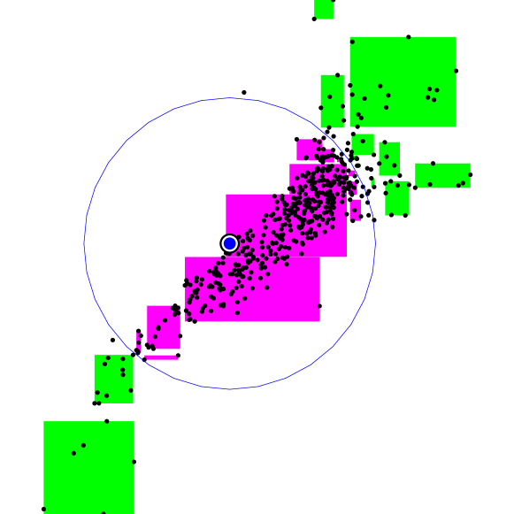
Figure 3: When doing a range count, nodes entirely within range can also be pruned and added to the total count. This additional pruning adds significant speed-ups to the slower range count discussed in Figure 2b. Now one just spends time studying nodes on the boundary of the range count.

4 Fast $N$–point Correlation Functions

4.1 The Single Tree Approach to Two-Point Computation

It is easy to see that the 2-point correlation function is simply a repeated set of range counts. For example, given a minimum and maximum separation ${\mbox{\it s}}_{lo}$ and ${\mbox{\it s}}_{hi}$ we run the following algorithm:

• $\mbox{\bf SingleTree2Point}(\mbox{\bf X},n,{\mbox{\it s}}_{lo},{\mbox{\it s}}_{hi})$
  Input X is a dataset, represented as a matrix in which the $k$th row corresponds to the $k$th datapoint. X has $R$ rows and $k$ columns. Input $n$ is the root of a kdtree built from the data in X. Output integer: the number of pairs of points $({\mbox{\bf x}}_{i},{\mbox{\bf x}}_{j})$ such that ${\mbox{\it s}}_{lo}\leq|{\mbox{\bf x}}_{i}-{\mbox{\bf x}}_{j}|<{\mbox{\it s}}_{hi}$.

• C := 0

• For $i$ between $1$ and $R$ do:

  • ${C}:={C}+\mbox{\bf RangeCount}(n,{\mbox{\bf x}}_{i},{\mbox{\it s}}_{hi})-\mbox{\bf RangeCount}(n,{\mbox{\bf x}}_{i},{\mbox{\it s}}_{lo})$

Note that in practice we do not use two range counts at each iteration, but one slightly more complex rangecount operation

$\mbox{\bf RangeCountBetweenSeparations}(n,\mbox{\bf q},{\mbox{\it s}}_{lo},{\mbox{\it s}}_{hi})$

that directly counts the number of points whose distance from q is between ${\mbox{\it s}}_{lo}$ and ${\mbox{\it s}}_{hi}$.

4.2 The Dual Tree Approach to Two-Point Computation

The previous algorithm iterates over all datapoints, issuing a range count operation for each. We can save further time by turning that outer iteration into an additional kd-tree search. The new search will be a recursive procedure that takes two nodes, ${n}_{\mbox{\scriptsize a}}$ and ${n}_{\mbox{\scriptsize b}}$, as arguments. The goal will be to compute the number of pairs of points $(\mbox{\bf x},\mbox{\bf y})$ such that $\mbox{\bf x}\in{n}_{\mbox{\scriptsize a}}$, $\mbox{\bf y}\in{n}_{\mbox{\scriptsize b}}$, and ${\mbox{\it s}}_{lo}\leq|\mbox{\bf x}-\mbox{\bf y}|<{\mbox{\it s}}_{hi}$.

• $\mbox{\bf DualTreeCount}({n}_{\mbox{\scriptsize a}},{n}_{\mbox{\scriptsize b}},{\mbox{\it s}}_{lo},{\mbox{\it s}}_{hi})$
  Returns an integer: the number of pairs of points $(\mbox{\bf x},\mbox{\bf y})$ such that $\mbox{\bf x}\in{n}_{\mbox{\scriptsize a}}$, $\mbox{\bf y}\in{n}_{\mbox{\scriptsize b}}$, and ${\mbox{\it s}}_{lo}\leq|\mbox{\bf x}-\mbox{\bf y}|<{\mbox{\it s}}_{hi}$.

• Let MinDist := the closest distance between ${{n}_{\mbox{\scriptsize a}}}.{\mbox{\scriptsize\sc BoundBox}}$ and ${{n}_{\mbox{\scriptsize b}}}.{\mbox{\scriptsize\sc BoundBox}}$.

• If $\mbox{\sc MinDist}\geq{\mbox{\it s}}_{hi}$ then it is impossible that any pair of points can match. So simply return 0.

• Let MaxDist := the furthest distance between ${{n}_{\mbox{\scriptsize a}}}.{\mbox{\scriptsize\sc BoundBox}}$ and ${{n}_{\mbox{\scriptsize b}}}.{\mbox{\scriptsize\sc BoundBox}}$.

• If $\mbox{\sc MaxDist}<{\mbox{\it s}}_{lo}$ then it is again impossible that any pair of points can match. So simply return 0.

• If ${\mbox{\it s}}_{lo}\leq\mbox{\sc MinDist}\leq\mbox{\sc MaxDist}<{\mbox{\it s}}_{hi}$ then all pairs of points must match. Use ${{n}_{\mbox{\scriptsize a}}}.{\mbox{\scriptsize\sc NumPoints}}$ and ${{n}_{\mbox{\scriptsize b}}}.{\mbox{\scriptsize\sc NumPoints}}$ to compute the number of resulting pairs ${{n}_{\mbox{\scriptsize a}}}.{\mbox{\scriptsize\sc NumPoints}}\times{{n}_{\mbox{\scriptsize b}}}.{\mbox{\scriptsize\sc NumPoints}}$, and return that value.

• Else, if ${n}_{\mbox{\scriptsize a}}$ and ${n}_{\mbox{\scriptsize b}}$ are both leaf nodes, we must iterate through all pairs of datapoints in their leaf lists. Return the resulting (slowly computed) count.

• Else at least one of the two nodes is a non-leaf. Pick the non-leaf with the largest number of points (breaking ties arbitrarily), and call it ${n}^{*}$. Call the other node ${n}^{-}$. Then:

  • Let ${C}_{\mbox{\scriptsize left}}:=\mbox{\bf DualTreeCount}({{n}^{*}}.{\mbox{\scriptsize\sc Left}},{n}^{-},{\mbox{\it s}}_{lo},{\mbox{\it s}}_{hi})$

  • Let ${C}_{\mbox{\scriptsize right}}:=\mbox{\bf DualTreeCount}({{n}^{*}}.{\mbox{\scriptsize\sc Right}},{n}^{-},{\mbox{\it s}}_{lo},{\mbox{\it s}}_{hi})$

  • Return ${C}_{\mbox{\scriptsize left}}+{C}_{\mbox{\scriptsize right}}$.

Computing a 2-point function on a dataset X then simply consists of computing the value $C=\mbox{\bf DualTreeCount}({n}_{\mbox{\scriptsize root}},{n}_{\mbox{\scriptsize root}},{\mbox{\it s}}_{lo},{\mbox{\it s}}_{hi})$, where ${n}_{\mbox{\scriptsize root}}$ is a kd-tree built from X, for a range of bins with minimum and maximum boundaries of ${\mbox{\it s}}_{lo}$ and $hisep$. We note here that the 2-point correlation function, the quanity of interest is not simply $C$, but $C/2$ (the number of unique pairs of objects).

A further speed–up can be obtained by simultaneously computing the $\mbox{\bf DualTreeCount}({n}_{\mbox{\scriptsize root}},{n}_{\mbox{\scriptsize root}},{\mbox{\it s}}_{lo},{\mbox{\it s}}_{hi})$ over a series of bins. We will discuss this in further detail in Connolly et al. (2001).

4.3 Redundancy Elimination

So far, we have discussed two operations – exclusion and subsumption – which remove the need to traverse the whole tree thus speeding–up the computation of the correlation function. Another form of pruning is to eliminate node-node comparisons which have been performed already in the reverse order. This can be done simply by (virtually) ranking the datapoints according to their position in a depth-first traversal of the tree, then recording for each node the minimum and maximum ranks of the points it owns, and pruning whenever ${n}_{\mbox{\scriptsize a}}$’s maximum rank is less than ${n}_{\mbox{\scriptsize b}}$’s minimum rank. This is useful for all-pairs problems, but will later be seen to be essential for all-k-tuples problems. This kind of pruning is not practical for Single-tree search.

4.4 Multiple Trees Approach to $N$–Point Computation

The advantages of Dual-Tree over Single-Tree are so far two fold. First, Dual-tree can be faster, and second it can exploit redundancy elimination. But two more advantages remain. First, we can extend the “2-tree for 2-point” method up to “N-trees for N-point”. Second (discussed in Section 5.1), we can perform effective approximation with Dual-trees (or n-trees). We now discuss the first of these advantages.

The $N$–point computation is parameterized by two $n\times n$ symmetric matrices: $L$ and $H$. We wish to compute

$$\sum_{i_{1}=1}^{R}\sum_{i_{2}=1}^{R}\ldots\sum_{i_{n}=1}^{R}I(L,H,i_{1},i_{2},\ldots i_{n})$$ (4)

where $I(L,H,i_{1},i_{2},\ldots i_{n})$ is zero unless the following conditions hold (in which case it takes the value 1):

$$\forall 1\leq i<j\leq n,{L}_{(i,j)}\leq|{\mbox{\bf x}}_{i_{i}}-{\mbox{\bf x}}_{i_{j}}|<{H}_{(i,j)}$$ (5)

We will achieve this by calling a recursive function FastNPoint on an $n$-tuple of kdtree nodes $({n}_{\mbox{\scriptsize 1}},{n}_{\mbox{\scriptsize 2}}\ldots{n}_{\mbox{\scriptsize n}})$. This recursive function much return

$$\sum_{i_{1}\in{n}_{\mbox{\scriptsize 1}}}\sum_{i_{2}\in{n}_{\mbox{\scriptsize 2}}}\ldots\sum_{i_{n}\in{n}_{\mbox{\scriptsize n}}}I(L,H,i_{1},i_{2},\ldots i_{n})$$ (6)

• $\mbox{\bf FastNPoint}({n}_{\mbox{\scriptsize a}},{n}_{\mbox{\scriptsize b}},{\mbox{\it s}}_{lo},{\mbox{\it s}}_{hi})$
  

• Let AllSubsumed:=TRUE

• For $i=1$ to $n$ do

  • For $j=i+1$ to $n$ do

    • Let MinDist := the closest distance between ${{n}_{\mbox{\scriptsize i}}}.{\mbox{\scriptsize\sc BoundBox}}$ and ${{n}_{\mbox{\scriptsize j}}}.{\mbox{\scriptsize\sc BoundBox}}$.

    • If $\mbox{\sc MinDist}\geq{H}_{(i,j)}$ then it is impossible that any $n$-tuple of points can match because the distance between the $i$th and $j$th points in any such $n$-tuple must be out of range. So simply return 0.

    • Let MaxDist := the furthest distance between ${{n}_{\mbox{\scriptsize i}}}.{\mbox{\scriptsize\sc BoundBox}}$ and ${{n}_{\mbox{\scriptsize j}}}.{\mbox{\scriptsize\sc BoundBox}}$.

    • If $\mbox{\sc MaxDist}<{L}_{(i,j)}$ then similarly return 0.

    • If ${L}_{(i,j)}\leq\mbox{\sc MinDist}\leq\mbox{\sc MaxDist}<{H}_{(i,j)}$ then every $n$–tuple has the property the the $i$th member and $j$th member match. We are interested in whether this is true for all $(i,j)$ pairs and so the first time we are disappointed (by discovering the above expression does not hold) then we will update the AllSubsumed flag. Thus the actual computation at this step is:

      If ${L}_{(i,j)}>\mbox{\sc MinDist}$ or $\mbox{\sc MaxDist}\geq{H}_{(i,j)}$ then
      AllSubsumed:=FALSE.

• If AllSubsumed has remained true throughout the above double loop, we can be sure that every $n$–tuple derived from the nodes in the recursive call must match, and so we can simply return

  $$\prod_{i=1}^{n}{{n}_{\mbox{\scriptsize i}}}.{\mbox{\scriptsize\sc NumPoints}}$$ (7)

• Else, if all of ${n}_{\mbox{\scriptsize 1}},{n}_{\mbox{\scriptsize 2}},\ldots{n}_{\mbox{\scriptsize n}}$ are leaf nodes we must iterate through all $n$–tuples of datapoints in their leaf lists. Return the resulting (slowly computed) count.

• Else at least one of the nodes is a non leaf. Pick the non-leaf with the largest number of points (breaking ties arbitrarily), and assume it has index $i=i^{*}$. Then:

  • Let ${C}_{\mbox{\scriptsize left}}:=\mbox{\bf FastNPoint}({n}_{\mbox{\scriptsize 1}},\ldots,{{n}_{\mbox{\scriptsize$i^{*}$}}}.{\mbox{\scriptsize\sc Left}},\ldots,{n}_{\mbox{\scriptsize n}})$

  • Let ${C}_{\mbox{\scriptsize right}}:=\mbox{\bf FastNPoint}({n}_{\mbox{\scriptsize 1}},\ldots,{{n}_{\mbox{\scriptsize$i^{*}$}}}.{\mbox{\scriptsize\sc Right}},\ldots,{n}_{\mbox{\scriptsize n}})$

  • Return ${C}_{\mbox{\scriptsize left}}+{C}_{\mbox{\scriptsize right}}$.

The full $N$–point computation is achieved by calling FastNPoint with arguments consisting of an $n$–tuple of copies of the root node.

We should note once again it is possible to save considerable amounts of computation by eliminating redundancy. For example, in the 4-point statistic, the above implementation will recount each matching 4-tuple of points $(x,y,z,w)$ in 24 different ways: once for each of the $4!$ permutations of $(x,y,z,w)$. Again, this excess cost can be avoided by ordering the datapoints via a depth-first tree indexing scheme and then pruning any $n$–tuple of nodes violating that order. But the reader should be aware of an extremely messy problem regarding how much to award to the count in the case that a subsume type of pruning can take place. If all nodes own independent sets of points the answer is simple: the product of the node counts. If all nodes are the same then the answer is again simple: ${n}\choose{N}$, where $n$ is the number of points in the node. Somewhat more subtle combinatorics are needed in the case where some nodes in the $n$-tuple are identical and others are not. And fearsome computation is needed in the various cases in which some nodes are descendants of some other nodes.

5 Controlled Approximation

In general, when the final answer comes back from FastNPoint, the majority of the quantity in the count will be the sum of components arising from large subsume prunes. But the majority of the computational effort will have been spent on accounting for the vast number of small but unprunable combinations of nodes. We can improve the running time of the algorithm by demanding that it also prunes it search in cases in which only a tiny count of $n$–tuples is at stake. This is achieved by adding a parameter, $T$, to the FastNPoint algorithm, and adding the following lines at the start:

• Let ${C}_{\mbox{\scriptsize max}}\mbox{\tt:=}\prod_{i=1}^{n}{{n}_{\mbox{\scriptsize i}}}.{\mbox{\scriptsize\sc NumPoints}}$

• If ${C}_{\mbox{\scriptsize max}}<T$ then quit this recursive call.

This will clearly cause an inaccurate result, but fortunately it is not hard to maintain tight lower and upper bounds on what the true answer would have been if the approximation had not been made. Thus $\mbox{\bf FastNPoint}({n}_{\mbox{\scriptsize 1}},{n}_{\mbox{\scriptsize 2}},\ldots,{n}_{\mbox{\scriptsize n}},T)$ now returns a pair of counts $({C}_{\mbox{\scriptsize lo}},{C}_{\mbox{\scriptsize hi}})$ where we can guarantee that the true count $C$ lies in the range ${C}_{\mbox{\scriptsize lo}}\leq C\leq{C}_{\mbox{\scriptsize hi}}$.

5.1 Iterative Deepening for Controlled Approximation

Suppose the true value of the $N$–point function is $C$ but that we are prepared to accept a fractional error of $\epsilon$: we will be happy with any value ${C}_{\mbox{\scriptsize approx}}$ such that

$$|{C}_{\mbox{\scriptsize approx}}-C|<\epsilon C$$ (8)

It is possible to adapt the n-tree algorithm using a best-first iterative deepening search strategy to guarantee this result while exploiting permission to approximate effectively by building the count as much as possible from “easy-win” node pairs while doing approximation at hard deep node-pairs. This is simply achieved by repeatedly calling the previous approximate algorithm with diminishing values of $T$ until a value is discovered that satisfies Equation 8.

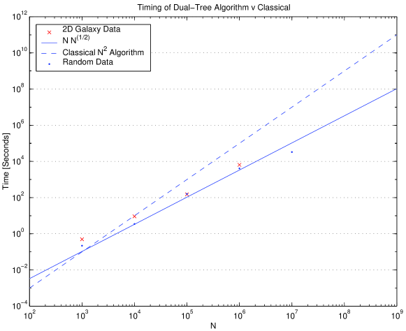
Figure 4: The computational time of our algorithm versus the size of dataset. The crosses are real 2-dimensional projected galaxy data while the dots are just drawn from a Poission distribution. The theoretically expected scaling law of $N\sqrt{N}$ is shown and agrees well with the observed data. The naive $N^{2}$ law is also plotted for comparison

6 Discussion

We plan to present a more detailed discussion of the techniques presented here in a forthcoming paper (Connolly et al. 2001). That paper will also include a full analysis of the computational speed and overhead of our $N$–point correlation function algorithm and compare those with existing software for computing the higher–order correlation functions e.g. Szapudi et al. 1999a. However, in Figure 4, we present preliminary results on the scaling of computational timing needed for a 2-point correlation function as a function of the number of objects in the data set. For these tests, we computed all the data–data pairs for random data sets and real, projected 2-dimensional galaxy data. These data show that our 2-point correlation function algorithm scales as $O(N\,\sqrt{N})$ (for projected 2-dimensional data) compared to the naive all-pairs scaling of $O(N^{2})$ where here $N$ is the size of the dataset under consideration. To emphasis the speed–up obtained by our algorithm (Figure 4), an all–pairs count for a database of $10^{7}$ objects would take only 10 hours (on our DEC Alpha workstation) using our methodology compared to $\sim 10,000$ hours ($>1$ year) using the naive $N^{2}$ method. Clearly, binning the data would also drastically increase the speed of analyses over the naive all–pairs $O(N^{2})$ scaling but at the price of lossing of resolution.

Similar spectacular speed–ups will be achieved for the 3 and 4–point functions and we will report these results elsewhere (Connolly et al. 2001). Furthermore, controlled approximations can further accelerate the computations by several orders of magnitude. Such speed–ups are vital to allow Monte Carlo estimates of the errors on these measurements. In summary, our algorithm now makes it possible to compute an exact, all–pairs, measurement of the 2, 3 and 4–point correlation functions for data sets like the Sloan Digital Sky Survey (SDSS). These algorithms will also help in the speed-up of Cosmic Microwave Background analyses as outlined in Szapudi et al. (2000).

Finally, we note here that we have only touched upon one aspect of how trees data structures (and other computer science techniques) can help in the analysis of large astrophysical data sets. Moreover, there are other tree structures beyond kd-trees such as ball trees which could be used to optimize our correlation function codes for higher dimensionality data. We will explore these issues in future papers.

References

- [1] Connolly, A. J., et al. 2001, in preparation
- [2] Friedman, J. H., Bentley, J. L., Finkel, R. A., 1977, Transactions on Mathematical Software, 3, 209
- [3] Gray, A., Moore, A. W., 2001, Proceedings of Advances in Neural Information Processing Systems 13.
- [4] Guttman, A., 1984, Proceedings of the Third ACM SIGACT-SIGMOD Symposium on Principles of Database Systems
- [5] Moore, A. W., Lee, M. S., 1998, Journal of Artificial Intelligence Research, 8
- [6] Moore, A. W., 2000, Proceedings of the Twelfth Conference on Uncertainty in Artificial Intelligence
- [7] Nichol, R. C., et al., 2000, proceedings from Virtual Observatories of the Future, Brunner& Szalay (astro-ph/0007404)
- [8] Peebles, P. J. E., 1980, The Large-Scale Structure of the Universe, Princeton University Press
- [9] Preparata, F. P., Shamos, M., 1985, Computational Geometry, Springer-Verlag
- [10] Scoccimarro, R., ApJ, see astro-ph/0004086
- [11] Szapudi, I., 2000, ApJ, see astro-ph/0010256
- [12] Szapudi, I., et al., 2000, ApJ, see astro-ph/0010256
- [13] Szapudi, I., et al., 1999a, ApJ, see astro-ph/0008131
- [14] Szapudi, I., et al., 1999b, ApJ, 517, 54
- [15] Uhlmann, J. K., 1991, Information Processing Letters, 40, 175
- [16] York, D., et al., 2000, AJ, 120, 1579
Index
- abstract *