Irregular Magnetic Fields in Interstellar Clouds and the Linear Polarization of Starlight

Abstract

Calculations are performed for the linear polarization of starlight due to extinction by aligned dust grains when the starlight traverses a medium with irregular magnetic fields. This medium is intended to represent the optically thick components of interstellar clouds which are observed to make little, if any, contribution to the polarization of starlight. In agreement with the observations, we find that the polarization properties of the starlight—the average fractional polarization and the dispersion in position angles—can be essentially unchanged. For this, the rms of the irregular component must be greater than the average magnetic field, which in turn tends to imply that the turbulent velocities in these interstellar clouds are super-Alfvénic.

1 Introduction

The fractional linear polarization of starlight tends to increase with extinction in the dilute, interstellar medium (ISM) as a result of the selective extinction by non-spherical dust grains which are aligned relative to the galactic magnetic field (e.g., Hiltner 1956). However, when the extinction occurs in the more dense medium of interstellar clouds, the increase in polarization with increasing extinction is noticeably reduced (Gerakines, Whittet, & Lazarian 1995; Goodman et al. 1995; but cf. Hough et al. 1988). When the starlight traverses clouds with visual extinctions (magnitudes) $A_{V}\approx 10$, the grains can have little if any effect on the polarization characteristics of the starlight. The reduced polarizing efficiency of grains has been observed to begin at an extinction $A_{V}=1$ to 2 (Arce et al. 1998; Harjunpää et al. 1999). This behavior has been interpreted as most likely due to the failure of the alignment mechanisms for the grains at the higher gas densities and optical depths. However, the widespread observation of linear polarization in the emission at far IR and submillimeter wavelengths by the grains in even more thick clouds (Hildebrand 1996) indicates that alignment mechanisms can be effective at the higher gas densities, at least under certain conditions.

An alternative interpretation is that the grains are aligned with the magnetic field, but that their contributions to the linear polarization nearly cancel because of rapidly changing directions of the grain alignment along the line of sight due to irregularities in the magnetic fields (e.g., Jones 1996). This interpretation has seemed to be incompatible with the requirement from the observations that both the fractional polarization and the dispersion in the position angles of the polarization can be essentially unchanged when the radiation traverses the cloud. We re-examine this conclusion by performing detailed calculations for the linear polarization of radiation that passes through an idealized medium which consists of dust grains that are aligned with irregular magnetic fields. Supersonic turbulent velocities are common in interstellar clouds (e.g., Crutcher 1999) and tend to indicate that turbulent magnetic fields must be present as well. Following Arons & Max (1975), irregular magnetic fields also have been widely discussed as playing a role in various aspects of the structure of interstellar clouds and in star formation.

2 Basic Methods

Representative, irregular magnetic fields are created by statistical sampling of the Fourier components of a power spectrum with the Kolmogorov (power law) form and with Gaussian distributions for the amplitudes. These methods are standard (e.g. Dubinski, Narayan, & Phillips 1995) and have been described in detail with our applications of them elsewhere (Watson, Wiebe, & Crutcher 2001; also, Wallin, Watson, & Wyld 1998). Based on the correlation function that we compute from available MHD simulations (see below), we utilize a power spectrum that is somewhat steeper than Kolmogorov (wavenumber $k^{-7/3}$ instead of $k^{-5/3}$). Two quantities enter to specify the magnetic fields created in this way—the rms value of a spatial component of the irregular magnetic field $B_{\rm rms}$ and the correlation length of these fields. We specify the latter in terms of the number of correlation lengths $N_{\rm corr}$ along an edge of the cubic volume of computational grid points in which the fields are created. A correlation length is specified here as the separation at which the structure function of the magnetic fields reaches essentially its asymptotic value (see Watson et al. 2001). Since the medium is assumed to be isotropic, $B_{\rm rms}$ will be the same along any one of the three orthogonal coordinate axes. The irregular magnetic field at each location is added to a constant, average magnetic field $\mbox{B}_{\rm avg}$ to create the total magnetic field. We restrict our attention to directions for $\mbox{B}_{\rm avg}$ that are perpendicular to the line of sight; this component is of most importance for linear polarization due to grains.

We also perform computations with magnetic fields that are the result of time-independent, numerical simulations by others for compressible MHD turbulence. We refer the reader to papers by these authors for a detailed description of the calculational methods (see Stone, Ostriker, & Gammie 1998). Certain basic aspects of the simulations are summarized in our earlier paper (Watson et al. 2001). Magnetic fields from two simulations will be utilized. In these simulations, the ratio $B_{\rm rms}/B_{\rm avg}$ is approximately 0.6 (medium) and 1.5 (weak), where the labels medium and weak refer to the relative strength of the average magnetic field. Both simulations have approximately the same supersonic turbulent velocities. The Mach number is about five. The ratio of the turbulent velocity to the Alfvén velocity (the Alfvénic Mach number) is 1.6 and 5, respectively, in the medium and weak field cases. For both simulations, we determine $N_{\rm corr}$ to be about twelve. Comparisons of the polarization computed with these MHD fields and with the statistically created fields provide an indication of the uncertainty in the calculations of the linear polarization to our approximate description of the irregular magnetic fields. The MHD simulations also contain information on the variation of the matter density and on its correlation with the variations in the magnetic field which are absent in our statistically created medium. Creating the magnetic fields by statistical sampling does, however, allow us to explore a wider range of values for $N_{\rm corr}$ and $B_{\rm rms}/B_{\rm avg}$. The cubic volumes used in the computations have 256 grid points on a side.

Stokes $Q$ and $U$ intensities describe the linear polarization of the radiation. When the fractional linear polarization $p\ll 1$ as is the case here, $Q$ and $U$ depend upon the integrals $q$ and $u$ where

$$q=\int\rho(s)\cos^{2}\gamma\cos 2\phi\,{\rm d}s$$ (1)

and the integral $u$ is obtained by replacing $\cos 2\phi$ by $\sin 2\phi$ in equation (1) [e.g., Lee & Draine 1985]. Here, the integration is along the distance $s$ of a straight-line path of a ray of starlight, $\rho(s)$ is the matter density, and $\gamma$ is the angle between the magnetic field and the plane of the sky. Except when we use the variations in density from the MHD simulations, $\rho(s)$ is taken as a constant. The angle $\phi$ is the angle between the projection of the magnetic field onto the plane of the sky and a reference axis in this plane. Then

$$p=(p/A_{V})_{\rm max}\,g\sqrt{q^{2}+u^{2}},$$ (2)

where $g$ is the factor (approximated here as a constant in the ISM) that relates the column density of matter to the optical extinction and $(p/A_{V})_{\rm max}$ is the maximum value of the ratio of the fractional linear polarization to the optical extinction. This maximum value is assumed to occur toward sources where the magnetic field, and hence the direction of the alignment of the dust grains, does not change along the line of sight. The position angle $\alpha$ of the linear polarization is ${\rm tan}^{-1}(u/q)/2$.

3 Application to Interstellar Clouds

The key observational information is that the characteristics of the linear polarization of the starlight that passes only through the intercloud medium and the periphery of an ISM cloud are observed to be essentially the same as the starlight that also passes through the more dense part of the cloud for clouds with $A_{V}$ of ten or so magnitudes. The calculations here will thus examine whether rays of starlight with a distribution of fractional polarizations and position angles similar to what is observed for the starlight at the periphery of a cloud can traverse a medium that is representative of the thick part of the cloud without these polarization characteristics being altered significantly. We examine this issue by utilizing the statistical sampling to create magnetic fields at the $(256)^{3}$ grid points in a cubic volume to represent the dense component of the cloud (the “dense cube”), and then performing the integrals to obtain $Q$ and $U$ for the $(256)^{2}$ rays that propagate along the grid lines of the cube. To create the $(256)^{2}$ rays with an initial distribution of fractional polarizations and position angles similar to that of the starlight which is observed at the periphery of the cloud, we first allow the rays to propagate through another cubic volume of magnetic fields (the “diffuse cube”). The properties of this diffuse cube ($N_{\rm corr}$, $B_{\rm rms}/B_{\rm avg}$ and the extinction $A_{V}$ through the cube) are chosen so that the rays emerge from it with the desired polarization characteristics. The parameters that describe the diffuse cube should not be viewed as additional “free parameters” since this cube is only a device for creating a distribution of rays with polarization characteristics similar to what is observed at the periphery of the cloud. It is noteworthy that choices for the diffuse cube which lead to rays with the desired average fractional polarization and dispersion in position angles are $B_{\rm rms}/B_{\rm avg}=0.6$ as inferred for the general ISM and the reasonable value $N_{\rm corr}=4.5$ (e.g., Jones, Klebe, & Dickey 1992).

The behavior of the average fractional polarization $\bar{p}_{\rm K}$ and the rms dispersion angle $\sigma_{\alpha}$ as the rays traverse the dense cube is shown in Figure 1. Since the observations are at K band, $(p_{\rm K}/A_{V})_{\rm max}=0.64$ % mag^-1 is used in equation (2). This value is computed from Serkowski (1973) law and multiplied by 1.4 from Mathis (1986). In the observations with which we are comparing, $\bar{p}_{\rm K}$ typically is about one percent and $\sigma_{\alpha}$ is 10–20 degrees for the starlight at the periphery of the cloud (Goodman et al. 1995). When the light that enters the cloud already is polarized, it is clear from Figure 1 that the change in $\bar{p}_{\rm K}$ and $\sigma_{\alpha}$ can be quite small if there are a number ($\gtrsim 12$) of correlation lengths across the dense cube and if $B_{\rm rms}$ is somewhat greater than $B_{\rm avg}$. The observational data reproduced in Figure 1 exhibit considerable scatter away from any single curve associated with a specific $N_{\rm corr}$ and $B_{\rm rms}/B_{\rm avg}$. This is not surprising. At any distance into the cube, the rays have a distribution of values for $p_{\rm K}$ for which typical values of one standard deviation are indicated by the error brackets in Figure 1. Results for computations in which the MHD fields (including variations in the density) are utilized for the dense cube also are indicated in the panels for $N_{\rm corr}=12$ which corresponds to the $N_{\rm corr}$ of the MHD simulations.

The variation of $p$ and $\sigma_{\alpha}$ in the dense cube is less than might be expected for a simple model of the medium consisting of a number ($N_{\rm corr}$) of independent cells along the path of the ray. This is partly because light that enters the dense cube is already polarized. The contributions to the integral in equation (1) from the diffuse and dense cubes will have opposite signs for approximately half of the rays when, for example, there is no average magnetic field. Such cancellations will tend to reduce the average increase of $p$. In addition, for turbulent magnetic fields, the integrand in equation (1) involves squares of three fields. It is quite irregular and is not well represented by $N_{\rm corr}$ identical cells.

In Figure 2, we relate our calculations to the issue of the minimum $A_{V}$ at which $(p/A_{V})$ begins to be reduced in ISM clouds. The reduction seems to begin at $A_{V}\approx 1$ and the total extinction in these observations is $A_{V}\approx 4$ to 5. Hence, we adopt $A_{V}=1$ and 3 for the diffuse and dense cubes, respectively, in the computations for Figure 1. Since the observations are centered around 7500Å (close to $V$), we adopt $(p_{V}/A_{V})_{\rm max}=4$ % mag^-1 (Mathis 1986) in equation (2). Results obtained when the MHD fields and density variations are substituted in the dense cube are again shown in the Figure. Clearly, the calculations are compatible with the observed variation of $\bar{p}_{V}$ with $A_{V}$ and with the requirement that $\sigma_{\alpha}$ ($\approx 20^{\circ}$) change by no more than a few degrees for the starlight from the segment of the Taurus cloud studied by Arce et al. (1998). As in Figure 1, at least several correlation lengths across the dense cube and a $B_{\rm rms}$ that is somewhat greater than $B_{\rm avg}$ are required.

4 Discussion

At least within the idealized treatment here, the conclusion that irregularities in the magnetic fields can allow the polarization characteristics $\bar{p}$ and $\sigma_{\alpha}$ to be relatively unaltered when starlight passes through the thick portion of ISM clouds depends upon only two parameters in the clouds—$N_{\rm corr}$ and $B_{\rm rms}/B_{\rm avg}$. Although we are not aware of good information on $N_{\rm corr}$ in ISM clouds, $N_{\rm corr}\gtrsim 10$ is a reasonable expectation (e.g., Myers & Goodman 1991). From the Figures, $B_{\rm rms}/B_{\rm avg}$ must then be greater than the ratio (1.5) for our weak field curve. In the MHD simulations with this ratio that we are utilizing, the corresponding rms turbulent velocity is about five times the Alfvén velocity. In MHD simulations more generally, the energy of the turbulent component of the magnetic field is about 0.3 to 0.6 of the turbulent kinetic energy (Vázquez-Semadeni et al. 2000). Super-Alfvénic turbulent velocities potentially have important implications for the MHD structure of interstellar clouds as emphasized by Padoan & Nordlund (1999) and later by MacLow (2001).

For some years, the observation of polarized emission in the far-IR and submillimeter has indicated that dust grains must commonly be aligned in dense, optically thick ISM clouds (e.g., Hildebrand 1996). It has, however, seemed that selection effects might reconcile the apparent conflict between these observations and the idea that the reduced effectiveness of grains to create polarization in extinction is a result of the failure of the alignment processes at higher optical depths. Observations of emission have tended to select warm grains which occur preferentially in environments with energy sources and are far from equilibrium, often in the vicinity of young massive stars. In these environments, the alignment mechanisms can be more effective (Lazarian, Goodman, & Myers 1997). However, polarized emission has recently been observed from dense, optically thick regions that also are quiescent (Clemens, Kraemer, & Ciardi 1999; Ward-Thompson et al. 2000; Vallée, Bastien, & Greaves 2000). It seems difficult to understand that the processes which align grains relative to the magnetic field should be more effective in these relatively quiescent regions than in the clouds where the reduction in the polarization caused by extinction is observed.

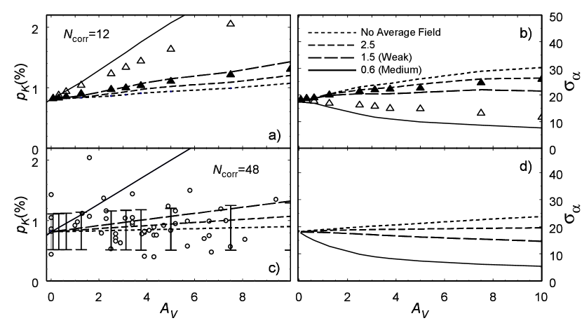
Figure 1: (panels a and c) The fractional polarization in the IR (K band) averaged over all rays $\bar{p}_{\rm K}$ versus optical extinction $A_{V}$ for starlight as it propagates through a medium that represents the thicker part of an ISM cloud. (panels b and d) The rms angle $\sigma_{\alpha}$ for the dispersions in the position angles of this linear polarization. Calculations are performed for several ratios $B_{\rm rms}/B_{\rm avg}$ of the irregular and average magnetic fields as indicated by the various line types. The panels differ according to the number of correlation lengths $N_{\rm corr}$ in the computational cube; $N_{\rm corr}=12$ for panels a and b, and $N_{\rm corr}=48$ for panels c and d. Calculations also are performed with magnetic fields and variations in the matter density obtained from the MHD simulations designated as “medium” and “weak” for which $B_{\rm rms}/B_{\rm avg}=0.6$ and 1.5, respectively. These results are indicated by open and filled triangles at several $A_{V}$ in panels a and b where $N_{\rm corr}=12$ is similar to that of the MHD simulations. The error brackets shown in panel c are representative for all curves in panels a and c, and indicate one standard deviation. Representative observational data from L1755 (Goodman et al. 1995) are designated by open circles in panel c.

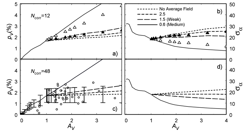
Figure 2: Similar meaning to Figure 1, except that here $\bar{p}_{V}$ and $\sigma_{\alpha}$ are shown as the rays of starlight first traverse a computational cubic volume which is intended to represent the diffuse periphery of the cloud before traversing the second computational cube which represents the thick part of the cloud. Representative observational data for $\bar{p}_{V}$ from a region in Taurus (Arce et al. 1998) are indicated by open circles in panel c. Error brackets indicating one standard deviation, and which are representative for all curves in panels a and c, are shown in panel c. The results of calculations utilizing the MHD fields and variations in the matter density are again designated by open and filled triangles in panels a and b.

References

- Arons & Max (1975) Arons, J., & Max, C. E. 1975, ApJ, 196, L77
- Arce et al. (1998) Arce, H. G., Goodman, A. A., Bastien, P., Manset, N., & Sumner, M. 1998, ApJ, 499, L93
- Clemens et al. (1999) Clemens, D., Kraemer, K., & Ciardi, D. 1999, in ESA-SP 435, Workshop on ISO Polarisation Observations, ed. R. J. Laureijs & R. Siebenmorgen, 7
- Crutcher (1999) Crutcher, R. M. 1999, ApJ, 520, 706
- Dubinski, Narayan, & Phillips (1995) Dubinski, J., Narayan, R., & Phillips, T. G. 1995, ApJ, 448, 226
- (6) Gerakines, P. A., Whittet, D. C. B., & Lazarian, A. 1995, ApJ, 455, L171
- Goodman et al. (1995) Goodman, A. A., Jones, T. J., Lada, E. A., & Myers, P. C. 1995, ApJ, 448, 748
- Harjunpää et al. (1999) Harjunpää, P., Kaas, A. A., Carlqvist, P., & Gahm, G. F. 1999, A&A, 349, 912
- Hildebrand (1996) Hildebrand, R. H. 1996, in ASP Conf. Ser. 97, Polarimetry of the Interstellar Medium, ed. W. G. Roberge & D. C. B. Whittet (San Francisco: ASP), 254
- Hiltner (1956) Hiltner, W.A. 1956, ApJS, 2, 389
- Hough et al. (1988) Hough, J. H., et al. 1988, MNRAS, 230, 107
- Jones (1996) Jones, T. J. 1996, in ASP Conf. Ser. 97, Polarimetry of the Interstellar Medium, ed. W. G. Roberge & D. C. B. Whittet (San Francisco: ASP), 381
- Jones et al. (1992) Jones, T. J., Klebe, D., & Dickey, J. M. 1992, ApJ, 389, 602
- Lazarian et al. (1997) Lazarian, A., Goodman, A. A., & Myers, P. C. 1997, ApJ, 490, 273
- Lee & Draine (1985) Lee, H. M., Draine, B. T. 1985, ApJ, 290, 211
- Mathis (1986) Mathis, J. S. 1986, ApJ, 308, 281
- McLow (2001) McLow, M.-M. 2001, in ASP Conf. Ser., The Orion Complex Revisited, ed. M. J. McCaughrean & A. Burkert (San Francisco: ASP), in press (astro-ph/9711349)
- Myers & Goodman (1991) Myers, P. C., & Goodman, A. A. 1991, ApJ, 373, 509
- Padoan & Nordlund (1999) Padoan, P., & Nordlund, Å. 1999, ApJ, 526, 279
- Serkowski (1973) Serkowski, K. 1973, in IAU Symp. 52, Interstellar Dust and Related Topics, ed. J. M. Greenberg & H. Ch. van de Hulst, 145
- Stone, Ostriker, & Gammie (1998) Stone, J. M., Ostriker, E. C., & Gammie, C. F. 1998, ApJ, 508, L99
- Vallée et al. (2000) Vallée, J. P., Bastien, P., & Greaves, J. S. 2000, ApJ, 542, 352
- Vázquez-Semadeni et al. (2000) Vázquez-Semadeni, E., Ostriker, E. C., Passot, T., Gammie, C. F., & Stone, J. M. 2000, in Protostars and Planets IV, ed. V. Mannings, A. P. Boss, S. S. Russell (Tucson: Univ. of Arizona Press), 3
- Watson et al. (2001) Watson, W. D., Wiebe, D. S., & Crutcher, R. M. 2001, ApJ, in press (astro-ph/0010276)
- Wallin et al. (1998) Wallin, B. K., Watson, W. D., & Wyld, H. W. 1998, ApJ, 495, 774
- Ward-Thompson et al. (2000) Ward-Thompson, D., Kirk, J. M., Crutcher, R. M., Greaves, J. S., Holland, W. S., & André, P. 2000, ApJ, 537, L135