Physical Parameter Eclipse Mapping

Abstract

The tomographic method Physical Parameter Eclipse Mapping is a tool to reconstruct spatial distributions of physical parameters (like temperatures and surface densities) in accretion discs of cataclysmic variables. After summarizing the method, we apply it to multi-colour eclipse light curves of various dwarf novae and nova-likes like VZ Scl, IP Peg in outburst, UU Aqr, V2051 Oph and HT Cas in order to derive the temperatures (and surface densities) in the disc, the white dwarf temperature, the disc size, the effective temperatures and the viscosities. The results allows us to establish or refine a physical model for the accretion disc. Our maps of HT Cas and V 2051Oph, for example, indicate that the (quiescent) disc must be structured into a cool, optically thick inner disc sandwiched by hot, optically thin chromospheres. In addition, the disc of HT Cas must be patchy with a covering factor of about 40% caused by magnetic activity in the disc.

1 Introduction

Cataclysmic variables (CVs) are close interacting binary system consisting of a main sequence star (the secondary) and a white dwarf. The Roche-lobe filling secondary loses matter via the inner Lagrangian point to the primary. If the magnetic field of the white dwarf is negligible, then angular momentum conservation drives the matter from the secondary into an accretion disc around the primary component. This disc matter is maintained by a steady mass stream from the secondary, which hits the disc in the so-called bright spot.

Some of these systems undergo frequently an outburst, in which the system brightens for a short period of time (a few days) in comparison to the interval between such eruptions (few weeks to months). It is believed that the accretion disc follows a disc instability cycle O in which the hydrogen in the disc switches its ionization status. Other systems, the so-called nova-like variables, appear to be in a permanent outburst state and are believed to exhibit optically thick, steady state discs. Quiescent disc, in contrast, show line emission, mainly of hydrogen and are therefore at least partially optically thin. An extensive overview over the theoretical and observational aspects of CVs is given in Warner W95 .

The ultimate wish of any astronomers is probably to be able to see the stars from close by, to get a direct image of the stellar systems. Tomographic methods give us a unique opportunity to get such a picture, even if indirect, without getting close to the object. By making use of the eclipse light curve, the classical Eclipse Mapping technique (EM, H85 ) provides us with images of the accretion disc, while Physical Parameter Eclipse Mapping (PPEM, VHH ) give us some insight into the accretion physics. This paper gives an introduction to PPEM and summaries applications of this method to multi-colour light curves of five different cataclysmic variables.

2 The PPEM method

Figure 1: Illustration of a cataclysmic variable going through an eclipse of the accretion disc. The parameters are set for IP Peg. Courtesy to K. Horne for the program cvmovie

Figure 1 illustrates the varying viewing angle a high inclination CV undergoes during an eclipse. One can see that at any one time during eclipse, only part of the accretion disc is occulted by the secondary. The flux at the given orbital phase is the total of all emission of any material not eclipsed at this phase. Any local intensity maximum in the accretion disc, e.g. the bright spot, will be eclipsed and reappears at a characteristic orbital phase and causes thereby a pair of steep gradients or steps in the observed eclipse light curve, one in ingress and the other in egress. Depending on the spatial location of this spot, the pair of steps will be shifted in relation to phase 0 which is defined as the conjunction of the white dwarf.

In EM one takes advantage of this spatial information of the intensity distribution of the accretion disc hidden in the eclipse profile. We have to make three basic assumptions: (a) the geometry of the secondary is known (it is usually a good approximation to assume it fills its Roche lobe); (b) the geometry of the disc is known (in the simplest approximation we use a geometrically infinitisimally thin disc); (c) the disc emission does not vary with time (this can be achieved by using averaged eclipse profiles in order to reduce the amount of flickering and flares from the disc). By fitting the eclipse light curve, we reconstruct the intensity distribution using a maximum entropy method (MEM, SB ). The MEM algorithm allows one to choose the simplest solution still compatible with the data in this otherwise ill-conditioned back projection problem. Further details of the EM method can be found in Horne H85 or Baptista & Steiner BS . The usefulness of this method is extensively described by R. Baptista in these proceedings.

Figure 2: A flowchart diagram to illustrate the Physical Parameter Eclipse Mapping algorithm

The PPEM approach goes a step further in that we map physical parameters, like temperature $T$ and surface density $\Sigma$, instead of intensities. Figure 2 explains the method by means of a flowchart diagram. In addition to the three above mentioned basic assumptions (indicated by the right upper panel) we have to presuppose a spectral model for the disc emission (indicated as “Model” in the chart), relating the parameters to be mapped (e.g. $T$, $\Sigma$) to the radiated intensity in a given filter (e.g. $I_{\nu}=f(T,\Sigma)$). The model can be as simple as a pure black body spectrum, the PPEM is then called Temperature Mapping or as complicated as non-linear LTE disc model atmospheres as calculated by Hubeny H91 . Two simple model spectra are described in Sect. 2.2. The predicted multi-colour light curves are then compared to the observed ones. As long as the fit is not satisfactory, the parameter maps are varied according to the MEM algorithm (i.e. using gradients $\delta I/\delta T$ (and $\delta I/\delta\Sigma$)). As soon as the $\chi^{2}$ that was aimed for is reached (and the maps have converged, see H85 ) the maps $T$ (and $\Sigma$) can be further analysed and compared to current disc models (see Sect. 4).

2.1 The light curves

The PPEM method requires input in the form of light curves. The number of light curves in various wavelength regions (filters/passbands) necessary to calculate a reliable parameter map depends on the used spectral model (see following Sect. 2.2) and must be equal to or greater than the number of parameters to be mapped. For example, if one uses a black body spectrum to map the temperature (see Sect. 5.2 or 5.1), one light curve would be sufficient for a unique PPEM analysis. However, the more light curves (in various filters) one uses the better: the long wavelength data (e.g. IR light curves) will be ideal to determine low temperature (outer) regimes in the disc, while the short wavelength data (e.g. UV light curves) will be most appropriate to map the hot (inner) disc regions.

If one uses an appropriate spectral model, such as calculated by Hubeny H91 , spectrophotometry can be analysed. PPEM ideally allows to extract a maximum of the information content of the data.

2.2 The model spectra

The spectral model provides a relation between the mapped parameter(s) $P$ and the intensity $I_{\nu}$ at the frequency $\nu$. If one would set $P=I_{\nu}$, this simply reduces PPEM to EM. In the simplest true PPEM version we use a black body spectrum for the spectral model, i.e.

$$I_{\nu}=B_{\nu}(T)=\frac{2h\nu^{3}}{c^{2}}\left(e^{\frac{h\nu}{kT}}-1\right)$$ (1)

which can be used to map the parameter temperature $T$ in the disc. Here $c$ is the speed of light, $h$ Planck and $k$ Boltzmann constant. Using this model we assume that the disc radiates optically thick. This option of the PPEM method is called Temperature Mapping and is useful for accretion discs in novae, nova-like variables and outbursting dwarf novae.

In order to allow the disc to be optically thin, as we expect in quiescent dwarf novae, we introduce a second parameter. We have some freedom in the choice, but since theoretical studies e.g. of the outburst behaviour use the surface density $\Sigma$ in the disc, we use the same. The next simple model thus is calculated as:

$$I_{\nu}=B_{\nu}(T)(1-e^{-\tau/\cos i})$$ (2)

with the optical depth

$$\tau=\rho\,\kappa\,2H,$$ (3)

where $\kappa$ is the mass absorption coefficient, $\rho$ the mass density

$$\rho=\Sigma\,/\,2H$$ (4)

and $H$ the disc scale height

$$H/R=c_{s}/V_{\mbox{\scriptsize kep}}.$$ (5)

Here, $R$ is the radius, $c_{s}=\sqrt{kT/(\mu m_{H})}$ is the local sound speed and $V_{\mbox{\scriptsize kep}}=\sqrt{G{\cal M}_{1}/R}$ the Keplerian velocity of the disc material, with $\mu$ the mean molecular weight, $m_{H}$ the mass of a hydrogen atom, $G$ the gravitational constant and ${\cal M}_{1}$ the mass of the white dwarf.

In our studies we used a pure hydrogen slab in local thermodynamic equilibrium (LTE) including only bound-free and free-free H and H^- emission. Even though this model is very simple it still is very useful in that it allows us to distinguish between optically thin and thick regions of the disc. The eclipse mapping of dwarf nova discs and the presence of emision lines suggest that at least part of the quiescent discs are optically thin.

For the usual range of temperatures and surface densities in CV accretion discs, this LTE approximation is still relatively good. In more realistic models (e.g. models by H91 ) one would include metals which significantly increase the opacity at temperatures lower than about $T_{\mbox{\scriptsize m}}\sim 6300$K leading to lower intensities than determined by our $I(T,\Sigma)$. Therefore, using our simple model, our algorithm overestimates the temperatures (and if optically thin also the surface density) in the cooler parts of the disc, in order to meet the required intensities. This will only be important in the outer regions of the disc with temperatures below $T_{\mbox{\scriptsize m}}$.

2.3 The white dwarf

For the white dwarf emission we used white dwarf spectra for the temperature range 10 000 K to 30 000 K. Outside this range black body spectra are used. The white dwarf is assumed as a spherical object in terms of occultation of the accretion disc and eclipse by the secondary, but it is attributed only a single temperature. Since the absorption lines partly coincide with the mean wavelengths of the filters, pass band response functions are used. Usually, the lower hemisphere of the white dwarf is assumed to be obscured by the inner disc.

2.4 The spatial grid for the accretion disc

In the present studies the accretion disc is assumed to be infinitesimally thin. Onto this disc we constructed a two-dimensional grid of pixel. This grid consists of rings cut into a number of pixel that provides equal areas for all pixel VHH . For reference of spatial structures in the disc, we use radius and azimuth. The radius is used in units of the distance between the white dwarf and the inner Lagrangian point $L_{1}$, the white dwarf being at the origin. The second coordinate is the azimuth, the angle as seen from the white dwarf and counting from $-180^{\circ}$ to $180^{\circ}$. Azimuth 0 points towards the secondary, the leading lune of the disc has positive and the following lune negative azimuth angles.

2.5 The uneclipsed component

Apart from the disc emission we allow for another emission component that is never eclipsed, e.g. the secondary. However, we do not need to specify a geometrical location or a spectral model for this uneclipsed component, but can reconstruct it for each wavelength/pass band independently as a constant flux contribution. It is usually given in the light curve plots as a solid horizontal line.

The uneclipsed component can then be used to give limits on the secondary or, if its contribution is known, the remaining uneclipsed flux can be analysed. It can originate in disc regions never eclipsed due to a relatively low inclination angle, or more likely regions at heights $z$ above the disc that are never eclipsed by the secondary.

2.6 The distance to the systems

In order to reconstruct sensible physical parameter distributions within the accretion disc, the distance to the system has to be known. Only in some cases, relatively good estimates could be made using e.g. the secondary absorption line spectrum or the white dwarf flux.

PPEM provides also the option to determine an independent estimate of the distance, using the combined flux of the accretion disc and the white dwarf. This estimate can either be compared to present estimates (e.g. HT Cas, UU Aqr) or give the first opportunity to establish a distance (e.g. V2051 Oph).

The PPEM distance estimate is based on the fact that a spectrum with at least 3 wavelength points is not only determined by the temperature and the surface density, but also by the distance. If the assumed distance is smaller or larger than the true distance, the fit to the data will be poor. In a multi-pixel analysis like PPEM this might be compensated by neighbouring pixel leading to an overall “good” fit to the observed light curve (expressed as a small $\chi^{2}$), but the resulting reconstruction will show artificial structures and the predicted light curve will have kinks not justified by the data. The amount of structure is expressed as the entropy $S$ of the map: the smoother the map the higher the entropy. For each trial distance $d$ we converge the maps to a specific $\chi^{2}$ and then plot the parameter $S$ against $d$. Where this function peaks, the map shows the least amount of structures and we will ideally find the true distance.

Only maps corresponding to fits of equal goodness can be compared for this distance estimate, since the entropy not only depends on the distance but also on the final $\chi^{2}$. The lower the $\chi^{2}$, i.e. the better the fit, the more structures will appear in the map, reducing thereby the entropy. At which $\chi^{2}$ to stop has to be determined individually, it depends on the goodness of the spectral model or the amount of flickering in the light curve and is therefore a somewhat subjective measure.

Using this distance estimate one presupposes that the spectral model describes the true emissivity of the disc reasonably well. It is difficult to determine the error introduced by a wrong model. A generally good fit to the observed multi-colour eclipse light curves, however, seems to justify the model used.

3 The reliability of the PPEM method

Figure 3: $\chi^{2}$ contours for different parameter combinations of temperature $T$ and surface density $\Sigma$ for a disc radius $R=0.32R_{\scriptscriptstyle L1}=1\cdot 10^{10}$ cm. For each parameter pair $T,\Sigma$ the spectrum $I(T,\Sigma)$ was calculated, then the spectra for $I(T\pm\Delta T,\Sigma\pm\Delta\Sigma)$ with small values for $\Delta T$ and $\Delta\Sigma$ and the difference in the spectra expressed as the $\chi^{2}$. Contours are drawn for $\chi^{2}=3$ and 1 assuming an error in the spectra of 1% of the maximum value. The narrower the contour line, the better determined the parameter.

Tests of the PPEM method were shown in Vrielmann et al.VHH . In general, the method allows to reconstruct the parameter distributions very well. However, it depends on the spectral model and the parameter values, how reliable the resulting maps are.

The black body spectrum is a non-linear function of the temperature, but since it gives an unambiguous function $I(T)$ it can be used to map the temperature uniquely. Therefore, the Temperature Mapping gives very reliable results. Since PPEM is using multi-colour light curves we see a huge improvement compared to classical eclipse mapping: steep gradients (e.g. at the disc edge) are much better reproduced in PPEM VHH .

For a $T-\Sigma$ model as described in Sect. 2.2 one has to check where in the parameter space the solutions $I(T,\Sigma)$ are unique before the maps can be reliably analysed. For example, in the optically thick limit (large $\Sigma$), the surface density can assume any value above a certain limit without a change in the spectrum. However, the temperature in this case is very well defined. In other regions of the parameter space only the surface density is well defined (large $T$, small $\Sigma$), in again other regions both (intermediate values of $T$ and $\Sigma$) or none (see the banana shaped contour lines for small $T$, small $\Sigma$ in Fig.3) of the parameters can be determined uniquely. This pattern changes slightly with the disc radius. Figure 3 shows this pattern for a radius of $R=0.32R_{\scriptscriptstyle L1}=1\cdot 10^{10}$ cm.

Parameters are most reliable in disc regions that emit the largest intensities. In disc regions with very low intensities the reconstructed parameters may be influenced by the MEM algorithm leading to a smoothing of the spatial gradients. This is typically the case in the outer disc regions.

Such a study can be used to derive error bars for the reconstructed temperature and surface density distribution. It is usually sufficient to determine these errors for azimuthally averaged maps as an indication for the reliability of the parameter values.

A useful tool to analyse the derived maps is the ratio of the averaged intensity distribution $I(T,\Sigma)$ to the black body intensity distribution $I_{BB}(T)$ derived from the temperature alone. In the optically thick case and for very low intensities this ratio reaches unity.

4 What to expect?

The reconstructed parameter distributions will allow us to calculate further parameters, like the optical depth, the disc scale height, the effective temperature and mass accretion rate or the viscosity. These gives us clues about the physics going on in the disc. What we can expect is described for the reconstructed and a few derived parameters.

4.1 The gas temperature

The gas temperature is expected to rise towards the disc centre. Close to the white dwarf the disc material is accelerated and the gravitational energy release is strongest. If the accretion disc emits as a black body, the gas temperature is equal to the effective temperature (see Sect. 4.3) and should decrease radially roughly like $T\sim r^{-3/4}$. In the optically thin case, the temperature distribution may be much flatter than this.

In case the disc has a hole, the reconstructed temperature values will decrease towards the disc centre below a value that is undetectable at the wavelengths used. However, if the hole is very small, MEM will lead to a smearing of the values resulting in a flat temperature distribution at small radii.

4.2 The surface density

The literature is divided about the radial behaviour of the surface density. While Meyer & Meyer-Hofmeister’s MM calculations result in a radially decreasing surface density distribution, Ludwig, Meyer-Hofmeister & Ritter LMR and Cannizzo et al. CGW derive slightly increasing surface density distributions.

Since the critical surface density distributions within the disc instability model show an increase of $\Sigma_{\mbox{\tiny crit}}$ with radius CW ; HLD we would rather expect that the actual $\Sigma(r)$ distribution also increases with radius. This would make it much easier for a disc to undergo an outburst.

Note, that if the disc is optically thick, we have no means to determine the surface density, only a lower limit that may be far from the true value.

4.3 The effective temperature

Considering the gravitational energy release and taking into account the slowing down of the disc material at the white dwarf surface, a steady state accretion disc should have the following radial effective temperature distribution FK :

$$T_{\mbox{\scriptsize eff}}(r)=T_{*}\left(\frac{r}{R_{1}}\right)^{-3/4}\left[1-\left(\frac{R_{1}}{r}\right)^{1/2}\right]^{1/4}$$ (6)

with

$$T_{*}=\left[\frac{3G{\cal M}_{1}\dot{\cal M}}{8\pi\sigma R_{1}^{3}}\right]^{1/4}$$ (7)

where $r$ is the radius in the disc, $R_{1}$ and ${\cal M}_{1}$ are the radius and mass of the white dwarf, $G$ the Gravitational constant, $\dot{\cal M}$ the mass accretion rate of the disc and $\sigma$ the Stephan-Boltzmann constant. For large radii Eq. (6) reduces to

$$T_{\mbox{\scriptsize eff}}(r)=T_{*}\left(\frac{r}{R_{1}}\right)^{-3/4}\,\,\,\,\mbox{for}\,\,\,\,r\gg R_{1}.$$ (8)

Deviations from this distribution in real disc show that it is not in steady state. This can be expected for a quiescent accretion disc of a dwarf nova awaiting the next outburst. Discs in nova-like variables and in outbursting dwarf novae are expected to follow the steady state $T_{\mbox{\scriptsize eff}}(r)$-profile.

4.4 The critical temperature

The effective temperature distribution can then also be compared to a critical temperature, as e.g. calculated by Ludwig et al. LMR . If the effective temperature distribution falls below this critical value the accretion disc is in the lower branch of the $T_{\mbox{\scriptsize eff}}-\Sigma$ hysteresis curve which is used to explain the disc instability cycle. Such a disc should undergo outbursts. If the temperatures are above this critical value, the accretion disc is on the hot branch of this hysteresis curve and should therefore be currently in outburst or within a nova-like or nova system.

4.5 The viscosity

A further parameter that can be derived is the viscosity $\nu$, usually parametrized as $\nu=\alpha c_{s}H$ (where $c_{s}$ is the local sound speed and $H$ again the disc scale height) using Shakura & Sunyaev’s SS $\alpha$-parameter. Theoretical studies involving the disc instability cycle predict values of $\alpha$ around 0.01 in quiescence S84 .

We calculate the viscosity using the standard relation between the viscously dissipated and total radiated flux $F_{\nu}$,

$$2H\alpha P\frac{3}{4}\Omega_{K}=\int F_{\nu}d\nu=\sigma T_{\mbox{\scriptsize eff}}^{4}$$ (9)

where $P$ is the (gas) pressure and $\Omega_{K}$the Keplerian angular velocity of the disc material.

5 Application to real data

This section gives some highlights of the application of the PPEM method to different objects. Any details about the analyses can be found in the corresponding, mentioned articles.

5.1 VZ Sculptoris

VZ Scl is a little studied eclipsing nova-like with an extreme difference between high (normal) and low states of about 4.5 mag OFW . Since in the low state the secondary dominates the spectrum at all wavelengths, Sherington et al. SBJ could determine a reliable distance of 530 pc. The other system parameters, in particular the inclination angle $i$ and the mass ratio $q$ are somewhat uncertain. We adopted the same values O’Donoghue et al. OFW used for their Eclipse Mapping and the ephemeris determined by Warner & Thackeray WT .

Figure 4: The temperature distribution of VZ Scl.

Our observations were according to O’Donoghue et al. OFW taken when the object was in its normal state and we therefore used the Temperature Mapping version of PPEM V99 . As expected, the black body assumption turned out to be a fairly good approximation. We reached a $\chi^{2}$ of 5. The disc appears to be in steady state between $0.15~{}R_{\scriptscriptstyle L1}$ to the disc edge at $0.7~{}R_{\scriptscriptstyle L1}$ with a mass accretion rate of about $3\times 10^{17}$gs^-1(see Fig. 4). In the inner part of the disc ($r<0.15~{}R_{\scriptscriptstyle L1}$) the temperature profile is very flat. This could be caused by a small hole in the disc, that is smeared out due to the MEM algorithm. Other explanations are discussed by e.g. Rutten et al. RvT , but the true cause is still not clear.

Note in particular, that we simply used the published distance and still achieved a relatively good fit to the data. In a future more extensive study we will test if the disc has optically thin region and if we can reach a better fit to the data using the $T-\Sigma$ version of PPEM. We will then also determine an independent distance estimate. However, we do not expect a great deviation from the literature value.

5.2 IP Pegasi

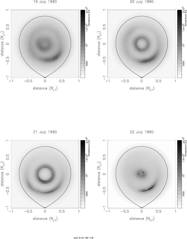
Figure 5: The temperature maps of IP Peg on decline from outburst. The secondary is always at the bottom, just outside the plotted area.

IP Peg is probably the best studied dwarf nova, and still is not completely demystified. It is most famous for the spiral waves found by Steeghs, Harlaftis, Horne (SHH , see also these proceedings) during rise to outburst.

We analysed UBVRI data taken during four nights on decline from outburst BHMW by feeding them into our PPEM algorithm V97 using the Temperature Mapping option. We achieved relatively good fits to the data, with $\chi^{2}$’s ranging between 1.1 and 4.

All four temperature maps (Fig. 5) show a prominent azimuthally smeared out bright spot at a radius of 0.5 to 0.55$R_{\scriptscriptstyle L1}$. The temperature in the central part, up to a radius of 0.1$R_{\scriptscriptstyle L1}$ drops dramatically during the three nights after maximum light from about 9 000 K to 4 000 K, possibly indicating an emptying out of the inner disc. Only in the last of the four nights, when the system reached the quiescent brightness, does the temperature reach again about 10 000 K at small radii. Instead, a hot ring at radius 0.2$R_{\scriptscriptstyle L1}$ present in the first three nights has disappeared in the last one. This mysterious behaviour seems to indicate that the outburst takes place only in the inner parts of the disc, without evidence of a cooling front.

These studies of VZ Scl and IP Peg during decline from outburst show that even the simple Temperature Mapping is a very useful tool.

Figure 6: Left: Averaged UBVRI light curves of UU Aqr in high state with the PPEM fits. The light curves are shifted upwards with the dotted line giving the zero line for each light curve. The residuals and the uneclipsed component are plotted in relation to the zero lines. Vertical dashed lines give the phases of the white dwarf ingress and egress. Right: Entropy vs. trial distance for $\chi^{2}=2.5$ (circles) and $\chi^{2}=2$ (triangles) and parabolic fits to the points peaking at 206 pc.

Figure 7: UU Aqr: Azimuthally averages of the reconstructed temperature (left) and surface density (right) distributions. The error bars give an indication of the reliability of the reconstructed values according to a study of the spectral model. In the inner part is the disc optically thick, therefore the surface density there gives only lower limits (indicated by triangles). In the outer regions, the intensity $I(T,\Sigma)$ becomes very small, leading to large error bars in $\Sigma$.

5.3 UU Aqarii

The eclipsing nova-like UU Aqr belongs to the SW Sex stars, i.e. in spite of the high inclination it shows single peaked emission lines with phase dependent absorption features. Doppler tomography reveals a disc, with the asymmetric part of the emission lines caused by a prominent bright spot HSSSB . This disc shows long term photometric variations in the form of high and low states with an amplitude of about 0.3 mag.

Baptista et al. BSC repeatedly observed UU Aqr over a period of about 6 years catching the system in a high and two low states. We applied the PPEM method to their averaged light curves separated in a high state and a low state light curve. Here, we present only the application of PPEM to the averaged high state data. An analysis of the averaged low state data (and of the individual light curves) will be presented by Vrielmann V20U .

Figure 6 (left) shows the averaged high state UBVRI light curves together with the PPEM fits. Baptista et al. BSC estimated a distance to UU Aqr by fitting the white dwarf fluxes. If the inner disc is opaque and obscures the lower hemisphere of the white dwarf, they derive a distance of $270\pm 50$ pc. Assuming an optically thick inner disc, Baptista et al. BSH performed a cluster main sequence fitting similar procedure to derive a distance of $200\pm 30$ pc.

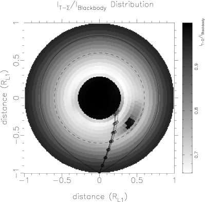
Figure 8: UU Aqr: Left: The azimuthally and spectrally averaged intensity ratio $I(T,\Sigma)/I_{BB}(T)$ as explained in Sect. 3 as a gray-scale plot. The dashed circle is the disc radius, the pear shaped line is the Roche-lobe of the primary and the lines from the inner Lagrangian point are ballistic stream lines for mass ratios $q\pm 50\%$. The secondary is at the bottom. Right: The radial effective temperature distribution. Underlying dotted lines are effective temperature distributions for steady state discs with mass accretion rates $\log\dot{\cal M}=13$ to 18, the one for $\dot{\cal M}=10^{16}$gs^-1 is drawn solid for reference. The dashed vertical line gives the disc radius, the dash-dotted line a critical temperature according to Ludwig et al. LMR

We independently estimated the distance to UU Aqr using the PPEM method as described in Sect. 2.6. Figure 6 (right) shows the entropy as a function of the trial distance. The parabolic fit to the data for $\chi^{2}=2$ peaks at a distance of 206 pc, consistent with Baptista et al.’s BSH estimate.

Fig. 7 shows the averages of the reconstructed temperature $T$ and surface density distributions $\Sigma$ with error bars indicating the reliablility of the reconstructed values. The derived intensity distribution $I(T,\Sigma)$ for the filter I helps us to define a disc radius. $I(T,\Sigma)$ has values at $r=0.6R_{\scriptscriptstyle L1}$ of less then 10% of the white dwarf value. In the outer regions the intensity vanishes and therefore the Balmer Jump disappears and the error bars of $\Sigma$ again become very large. For large radii, the temperature drops below $T_{\mbox{\scriptsize m}}$, i.e. the true temperatures are even lower and reach undetectable limits. Finally, the original $T,\Sigma$ maps show a bright spot at a radius of $r_{\mbox{\footnotesize spot}}=0.6R_{\scriptscriptstyle L1}$ (see also Fig. 8, left) which lets us set the disc size as $0.6R_{\scriptscriptstyle L1}$.

While the temperatures are everywhere well defined and decrease with radius as expected, the surface density values are only in the outer parts of the disc ($0.3R_{\scriptscriptstyle L1}<r<0.6R_{\scriptscriptstyle L1}$) trustworthy. They clearly increase with radius even within the allowance of the error bars. In the inner part the disc is optically thick (see Fig. 8, left) and we can only derive lower limits for $\Sigma$. The true values, however, may be much larger than those limits.

The white dwarf temperature was reconstructed to 26 100 K using white dwarf spectra as described in Sect. 2.3. This value very well lies in the usual range of white dwarf temperature estimates of between 9 000 K and 60 000 K S98 and quite close to the average effective temperatures of white dwarfs in non-magnetic CVs, $<T_{\mbox{\scriptsize eff}}>=24\,100$ K  S99 .

As Fig. 8 (left) shows, only the central region up to about $0.3R_{\scriptscriptstyle L1}$ is optically thick, the remaining disc is optically thin, including the bright spot. This is unexpected, nova-likes are expected to have overall optically thick discs. However, this indicates a probable location for the line emission, i.e. in the outer parts of the disc.

The gray-scale plot shows that the bright spot is relatively weak compared to Hoard et al.’s HSSSB Doppler maps and delayed in the disc with respect to the expected position, where the ballistic stream hits the accretion disc. The stream matter apparently enters the disc in such a way that it first travels with the rotating material in the disc before it releases and radiates its energy away. It coincides possibly with Hoard et al.’s absorbing wall, where the line emission diminishes because the material is nearly optically thick.

Baptista et al. BSC estimate of the mass and radius of the secondary fits to a main sequence star in the range M3.5 to M4. Subtracting the flux of such a star from the uneclipsed component requires the object to be later than about M3.7. Such a star would leave us with no significant flux in I and a spectrum that rises towards shorter wavelenghts and peaks in the B filter. It is not possible to fit a black body spectrum to this distribution. The uneclipsed flux must therefore originate in an extended, possibly optically thick region with varying temperature. Contrary to HT Cas (Sect. 5.5) and V2051 Oph (Sect. 5.4), there is no cool component of the uneclipsed flux.

Further details concerning this study including an analysis of all of Baptista’s individual light curves in high and low states will appear in Vrielmann V20U . This presented study shows in particular, that our PPEM analysis gives results in agreement with other methods, especially concerning the distance to the system.

Figure 9: Left: Averaged UBVRI light curves of V2051 Oph with the PPEM fits. For the explanation of the dashed and dotted lines see Fig. 6 (left). Right: Entropy vs. trial distance for $\chi^{2}=3$ and a parabolic fit to the points peaking at 154 pc

5.4 V2051 Ophiuchi

The nature of the cataclysmic variable V2051 Oph was mysterious since the discovery by Sanduleak S72 . It has been classified as a (low-field) polar BW where the orbital hump is explained as a flaring accretion column WO and as a dwarf nova showing outbursts, double peaked emission lines and an eclipse light curve that can be explained as caused by an accretion disc BCHZ ; WC ; WBHGMC .

Figure 10: V2051 Oph: The averaged reconstructed temperature (left) and surface density (right) distributions with error bars according to a study of the model. The error bars therefore indicate the reliability of the reconstructed parameter values, not the variation in azimuth. The values at intermediate radii ($0.2R_{\scriptscriptstyle L1}$ to $0.4R_{\scriptscriptstyle L1}$) have been split up to illustrate the range of parameter values. At a radius of 0.04$R_{\scriptscriptstyle L1}$ the disc is completely optically thick, i.e. we omitted its reconstructed $\Sigma$ value. For the next two annulli the disc is nearly optically thick, therefore we only give a lower limits for the surface density, indicated by a triangles.

It is certain that it is a high inclination system, displaying eclipses and double peaked emission lines and after the super outbursts in May 1998 and July 1999 it seems clear that the system must have an accretion disc. Warner W96 suggested that it might be the first system of a new class he terms polaroid. Polaroids are similar to intermediate polars (IPs), i.e. dwarf novae in which the white dwarf has an intermediately strong magnetic field that disrupts the inner part of the disc. However, while IPs have a fast spinning white dwarf, the primary in a polaroid is synchronized.

Figure 9 (left) shows UBVRI light curves of V2051 Oph averaged over eight eclipses and as used in the PPEM analysis of Vrielmann V20V . Most flares and the flickering are averaged out, except for the originally strong flare at phase 0.12.

We used the PPEM method to establish the first reliable distance estimate to V2051 Oph as described in Sect. 2.6. For each trial distance the data have been fitted to a $\chi^{2}$ of 3. Figure 9 (right) shows the resulting entropy as a function of trial distance. A parabolic fit to the data points peaks at 154 pc.

Figure 10 shows averages of the reconstructed temperature and surface density distribution with error bars according to a study of the model. The values in the radial region $0.2R_{\scriptscriptstyle L1}$ to $0.4R_{\scriptscriptstyle L1}$ have been split up in an upper and lower branch because of a true spatial separation of regions and to illustrate the range of reconstructed parameters as well as that of the error bars. The upper branch values in both parameters correspond to a relatively confined region in the disc that we call hot region. It is located between the stars and is nearly optically thick. The lower branch values correspond to the remaining disc (cf. Fig. 11, left). In the outer regions of the disc the error bars in both parameters increase, because the parameter values enter the region with banana shaped $\chi^{2}$ contour lines (see Fig. 3).

The temperature $T$ decreases radially, as expected. In contrast, the surface density $\Sigma$ rises towards the disc edge, but according to the large error bars in the outer disc regions, $\Sigma$ could also be almost constant throughout the disc. However, a decrease of $\Sigma$ with radius appears out of the question.

Using white dwarf spectra, the white dwarf temperature was reconstructed to 22 700 K. This value is close to typical values of white dwarf temperatures, but somewhat higher than in the similar objetcs HT Cas, OY Car and Z Cha of around 15 000 K GK .

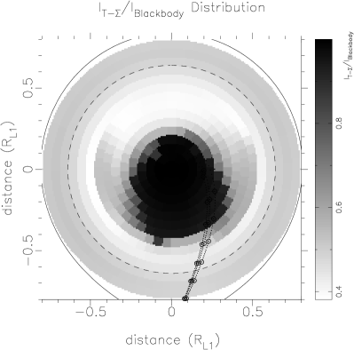
Figure 11: V2051 Oph: Left: The ratio $I(T,\Sigma)/I_{BB}(T)$ as a gray-scale plot. Right: The radial effective temperature distribution. The dashed and dotted lines in both plots have the same meaning as in Fig. 8

Figure 11 (left) gives a gray-scale display of the spatial distribution of the ratio $I(T,\Sigma)/I_{BB}(T)$. The central parts up to a radius of $0.15R_{\scriptscriptstyle L1}$ and the hot region between the stars are optically thick. In the outer region, $I(T,\Sigma)/I_{BB}(T)$ is close to unity, because both $I(T,\Sigma)$ and $I_{BB}(T)$ vanish there. Part of the optically thick hot region can be attributed to the bright spot, expected at the point where the ballistic gas stream hits the disc. But the hot region is too large and spreads out too far towards negative azimuths (into the following lune).

The right panel of Fig. 11 shows the radial distribution of the effective temperature in V2051 Oph’s disc. A clear separation can be seen for the hot region and the remainder of the disc. While the mass accretion rate $\dot{\cal M}$ of the hot region lies above the critical value, the remaining disc’s $\dot{\cal M}$ is approximately equal to the critical value or below. Since V2051 Oph is a dwarf nova showing occational outbursts, this mass accretion rate is far too high. It should lie well below the critial value.

A grayscale plot of the $T_{\mbox{\scriptsize eff}}$ distribution (not shown here) shows a distinct ridge within the hot region. It is almost parallel to the binary axis, but tilted by about 15^∘ towards the following lune of the disc.

In order to explain the hot region, the presence of an outbursting disc and the variable humps as seen by Warner & O’Donoghue WO we propose the model for V2051 Oph as described in Sect. 6.1.

Calculating the viscosity parameter $\alpha$ we derive values far too large. While theory predicts values in the range of $\alpha\sim 0.01$ (see Sect. 4.5), our values lie between 30 and 1000. In Sect. 6.2 we explain how we can solve this discrepancy with our proposed model of accretion discs.

The uneclipsed component is reconstructed to 0.56 mJy, 0.43 mJy, 0.00 mJy and 0.66 mJy for the filters UBVR, respectively. Baptista et al.’s BCHZ mass and radius for the secondary, fits to a M4.5 main sequence star KM , however, this leads to fluxes of 0.07 mJy in V and 0.22 mJy in R. The secondary must therefore be of slightly later type or the error in the reconstructed values is of order a few hundredth mJy.

The separation of the UV and IR component means the uneclipsed component must originate in two separate sources. The UV flux probably comes from the hot chromosphere, extending to at least a few white dwarf radii above the disc plane. The IR source may be a cool disc wind. These estimates, though, are only valid as long as the spectral model is a good representation of the true emissivity of the disc.

Any further details about this analysis are described in Vrielmann V20V .

5.5 HT Cassiopeiae

HT Cas is an unusual dwarf nova in that it does not show much of a bright spot and has occationally very long quiescent times of up to 9 years. On the other hand, Patterson P suggested it might serve as a Rosetta stone in explaining what drives the accretion discs. Since it is one of the few eclipsing dwarf novae it gives us a special opportunity for the analysis of a quiescent disc with PPEM.

Figure 12: Left: Averaged UBVRI light curves of HT Cas with the PPEM fits. For the explanation of the dashed and dotted lines see Fig. 6 (left). Right: Entropy vs. trial distance for $\chi^{2}=1.75$ and a parabolic fit to the points peaking at 207 pc

We used UBVR light curves previously analysed and published by Horne et al. HWS . Figure 12 (left) shows the averaged UBVR eclipse light curves as prepared for our PPEM analysis VHH2 . Most of the flickering has disappeared and the most prominent remaining feature is the white dwarf eclipse.

We used these data to determine an independent distance estimate as described in Sect. 2.6. Previous reliable estimates involved the secondary M and the white dwarf WNHR and resulted in values of 140 pc and 165 pc, respectively. Our PPEM estimate is significantly larger with a value of 207 pc (Fig. 12, right), however, the fits to the light curves are very good with a $\chi^{2}$ of 1.75. Sect. 6.3 describes our suggested solution for this distance problem. It allows us to use the parameter values as reconstructed.

Figure 13: HT Cas: The averaged reconstructed temperature (left) and surface density (right) distributions with error bars according to a study of the model

Figure 13 gives azimuthally averaged temperature and surface density distributions as reconstructed for the trial distance 205 pc. Like in the disc of V2051 Oph, the temperature decreases with radius. However, the surface density clearly increases radially even within the large error bars. The corresponding intensity distribution allow us to set a radius of the disc at $0.4R_{\scriptscriptstyle L1}$.

The reconstructed temperature of the white dwarf is 22 600 K. Because of our larger distance, this value is larger than Wood et al.’s WNHR value of $18\,700\pm 1\,800$ K determined from the same data.

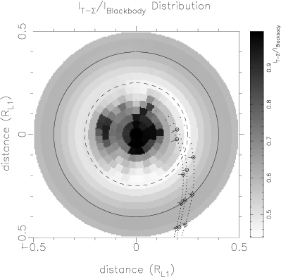
Figure 14: HT Cas: Left: The ratio $I(T,\Sigma)/I_{BB}(T)$ as a gray-scale plot. The solid circle is the disc radius, the dashed circle indicates where the surface density values become uncertain. The Roche-lobe of the primary lies entirely outside the displayed area. Otherwise same as Fig. 8 (left). Right: The radial effective temperature distribution for a distance of 205 pc (circles) and 133 pc (dots). The dashed vertical line gives the radius where the surface density values become uncertain and the solid line gives the disc radius. Otherwise same as Fig. 8 (right)

As shown by Fig. 14 (left), only the very central parts of the accretion disc are optically thick and the $I(T,\Sigma)/I_{BB}(T)$ ratio shows some asymmetry, also present in the original $T-\Sigma$ maps. We would expect the emission lines to originate only in regions of the disc with radii $r>0.05R_{\scriptscriptstyle L1}$.

Assuming a distance of 205 pc, the effective temperature is significantly larger than the critical values (see Fig. 14, right). It would be difficult to explain such high effective temperature and therefore mass accretion rates in a system that shows only rare outbursts, i.e. should have an exceptionally low mass accretion rate. If we agree with the cited literature values for the distance and assume a distance of 133 pc (see Sect. 6.3), the effective temperature would drop to values below or close to the critical temperatures also shown in Fig. 14 (right). In the inner part of the disc ($r<0.2R_{\scriptscriptstyle L1}$), the $T_{\mbox{\scriptsize eff}}$ is flat, while outside this range the disc is steady state like with a mass accretion rate of about $2\times 10^{15}$gs^-1.

Similarly as in the case of V2051 Oph, the viscosity parameter $\alpha$ we determine from the maps using Eq. (9) assumes values too large by three to four orders of magnitude. Sect. 6.2 describes our model for the disc in both systems which qualitatively explains our solution of the discrepancy to theory.

The reconstructed uneclipsed component can partly be explained by a M5.4 secondary M . Subtracting such a main sequence star using a distance of 133 pc, basically no extra uneclipsed flux in the V band remains, like in V2051 Oph. However, in U, B, and R we find significant additional flux of 0.1 mJy, 0.08 mJy, and 0.05 mJy, respectively. As in V2051 Oph this must originate from two distinctly different sources, presumeably a hot chromosphere (providing the U and B flux) and a cool disc wind, giving rise to the R flux.

6 Discussion

6.1 About the nature of V2051 Oph

V2051 Oph has often been compared to HT Cas, OY Car and Z Cha because of the similar orbital periods and all being SU UMa stars. Especially the similarly long and similarly variable outburst intervals of HT Cas and V2051 Oph is striking. One would hope that if one could explain one of these objects, all were understood.

However, V2051 Oph has some special features, like the variable hump as seen in the light curves of Warner & Cropper WC and Warner & O’Donoghue WO that can only be explained by a hump source very close to the white dwarf. Objects with an (disrupted) accretion disc and an (flaring) accretion column would most easily be explained as an intermediate polar (IP). However, IPs usually show characteristic X-ray emission. V2051 Oph has only been detected as a very faint X-ray source, but on the other hand no high inclination system shows high X-ray count rates. Instead there seems to exist an anti-correlation between the observable X-ray emission measure and the inclination angle. The X-ray source therefore is very close to the white dwarf and must be obscured or absorbed in the high inclination systems HCP ; vBV .

The absence of circular polarisation in the wavelength range 3500-9200 ÅC could be explained by a very low magnetic field of 1 MG or less WO , as expected for IPs.

If V2051 Oph is indeed an intermediate polar, the inner disc radius must be very small, of order less than $0.1~{}R_{\scriptscriptstyle L1}$. Otherwise, it would have been reconstructed by PPEM. On the other hand, the accretion curtains would partially fill out the space between the white dwarf and the accretion disc.

Warner W96 suggests that V2051 Oph could be one of the systems he terms polaroid. A polaroid is an intermediate polar with a synchronized white dwarf. With our analysis we cannot distinguish between an IP and a polaroid, but oscillation found in V2051 Oph indicate a non-synchronous white dwarf S20 and therefore we favour the IP model.

It remains to be explained what causes the hot region in the disc. One possibility is limb brightening of the accretion disc that we did not take into account. If the disc was flared this effect would even be enhanced. However, it would not explain the slightly asymmetric ridge we see in the effective temperature distribution. Another possibility is an illumination from a bulge where the ballistic stream hits the accretion disc as described in Buckley & Tuohy BT . However, this would also make it difficult to explain the ridge in the effective temperature map. A third explanation is a warp in the disc in such a way that the disc region between the stars is illuminated by the white dwarf at azimuths $-15^{\circ}$ and the region on the opposite side of the disc ($+165^{\circ}$) has a bulge so that the outer parts of the disc cannot be illuminated by the central object (for a more detailed explanation see V20V ). However, it would be difficult to explain if it is stable in the rotating frame of the binary.

A PPEM analysis of multi-colour light curves from other time periods would be helpful in deciding what causes the hot region, if its location in the disc is stable, rotates in the disc or is variable in its presence.

6.2 Accretion Disc model for HT Cas and V2051 Oph

Instead of dismissing Eq. (9) or our PPEM analysis altogether, we were seeking for an explanation for the high values of $\alpha$ of a few hundreds that we derive for the disc in both HT Cas and V2051 Oph.

If we compare our derived surface density values with the values used in the disc instability model FLP ; LMR ; S82 we find that our values are much lower than those necessary for the disc entering the hysteresis curve. Theory predicts values between 10 and 100 g cm^-2 for $\alpha$’s between 0.1 and 1 and even at larger $\Sigma$’s for smaller $\alpha$’s. Since the disc cannot change the $\Sigma$ from quiescence to outburst that dramatically, this means the outburst can only occur if the disc is very well optically thick already before its onset. On the other hand line emission is seen during rise and decline of an outburst HRNZ .

To solve this problem we suggest that the disc consists of a cool, optically thick layer carrying most of the matter and which is sandwiched by a hot, optically thin chromosphere. The surface densities in the underlying disc must be a factor $10^{4}$ ($\Sigma$ a few hundreds) larger then the reconstructed values to bring the $\alpha$’s down to reasonable values of between 0.01 and 0.1. However, we only “see” the chromosphere, therefore we derive the large values for $\alpha$.

The presence of a hot chromosphere is supported by the excess of blue emission in the uneclipsed component in HT Cas, V2051 Oph and UU Aqr. This emission must come from regions above the disc plane that are never eclipsed, i.e. a few white dwarf radii. This means, the chromosphere is an extended layer on top of the disc surface. Furthermore, this chromosphere must be the location where the line emission originates.

6.3 HT Cas’ patchy disc

In a similar way as above, the distance problem with HT Cas does not mean we have to dismiss the PPEM algorithm right away. As we have shown, the PPEM estimate gives results in agreement with literature values for UU Aqr (see Sect. 5.3). Furthermore, our use of literature values for IP Peg and VZ Scl does not indicate any disagreement.

Instead, we can explain our large discrepancy between our PPEM distance estimate and literature values for HT Cas by allowing the disc to be patchy, i.e. the emitting surface is smaller then the geometrical surface. Using Marsh M distance estimate with a recalibrated Barnes-Evans relation (for details see VHH2 ), the covering factor must be of the order $C=(133/207)^{2}=41$%.

The patchy disc can be caused by magnetic activity in localized regions on the surface or in the upper layers of the accretion disc. Magnetic flux created by dynamo action and/or the Balbous-Hawley instabilities driving the viscosity rises out of the cool midplane regions and dissipates most of the viscously generated energy via magnetic reconnection or similar coronal processes. This model also explains why the energy dissipation rate is proportional to the local orbital frequency HS .

Our PPEM analysis of HT Cas gives an indirect evidence of the hydromagnetic nature of the anomalous viscosity in accretion disks.

7 Summary

We have shown that Physical Parameter Eclipse Mapping is a powerful tool that helps us to learn about the physics of accretion discs in cataclysmic variables. This review can only highlight some interesting results. But, whether we derive “just” an independent distance estimate or get insight into the disc structure, there is always something to learn from the application of this method.

References

- (1) Baptista R., Steiner J.E., 1993, A&A 277, 331
- (2) Baptista R., Steiner J.E., Cieslinski, D., 1994, ApJ, 433, 332
- (3) Baptista R., Steiner J.E., Horne K., 1996, MNRAS, 282, 99
- (4) Baptista R., Catalán M.S., Horne K., Zilli D., 1998, MNRAS, 300, 233
- (5) Bobinger A., Horne K., Mantel K.-H., Wolf S., 1997, A&A 327, 1023
- (6) Bond H., Wagner R.L., 1977, IAU Circ. 304
- (7) Buckley D.A.H., Tuohy I.R., 1989, ApJ, 344, 376
- (8) Cannizzo, J.K., Wheeler J.C., 1984, ApJS, 55, 367
- (9) Cannizzo J.K., Gosh P., Wheeler J.C., 1982, ApJ, 260, L83
- (10) Cropper M.S., 1986, MNRAS, 222, 225
- (11) Faulkner J., Lin D.N.C., Papaloizou J., 1983, MNRAS, 205, 359
- (12) Frank J., King A., Raine D., 1992, In: “Accretion Power in Astrophysics”, Cambridge Astrophysics Series, Cambridge University Press, p. 81
- (13) Gänsicke, B.T., Koester, D. 1999, A&A, 346, 151
- (14) Hameury J.-M., Lasota J.-P., Dubus G., 1999, MNRAS, 303, 39
- (15) Hessman F.V., Robinson E.L., Nather R.E., Zhang E.-H., 1984, ApJ, 286, 747
- (16) Hoard D.W., Still M.D., Szkody P., Smith R.C., Buckley D.A.H., 1998, MNRAS, 294, 689
- (17) Holcomb S., Caillault J.-P., Patterson J., 1994, A&AS, 185, 2117
- (18) Horne K., 1985, MNRAS, 213, 129
- (19) Horne K., Saar S.H., 1991, ApJ, 374, L55
- (20) Horne K., Wood J.H., Stienning R.F., 1991, ApJ, 378, 271
- (21) Hubeny I., 1991, In: IAU Colloq. 129, “Structure and Emission Properties of Accetion Disks”, eds. C. Bertout, S. Collin, J.-P. Lasota, J. Tran Thanh Van (Singapure: Fong & Sons), p. 227
- (22) Kirkpatrick, J.D., McCarthy, D.W. 1994, AJ, 107, 333
- (23) Ludwig K., Meyer-Hofmeister E., Ritter H., 1994, A&A 290, 473
- (24) Marsh T.R., 1990, ApJ, 357, 621
- (25) Meyer F., Meyer-Hofmeister E., 1982, A&A, 106, 34
- (26) O’Donoghue, D., Fairall, A.P., Warner, B. 1987, MNRAS, 225, 43
- (27) Osaki Y., 1996, PASP, 108, 39
- (28) Patterson J., 1981, ApJS 45, 517
- (29) Rutten R.G.M., van Paradijs J., Tinbergen J., 1992 A&A, 260, 213
- (30) Sanduleak N. 1972, IBVS, No. 663
- (31) Shakura N.I., Sunyaev R.A., 1973, A&A, 24, 337
- (32) Sherington M.R., Bailey J., Jameson R.F., 1984, MNRAS, 206, 859
- (33) Sion E.M., 1999, PASP, 111, 532
- (34) Skilling J., Bryan R.K., 1984, MNRAS 211, 111
- (35) Steeghs D., 2000,private communication
- (36) Steeghs D., Harlaftis E.T., Horne K., 1997, MNRAS, 290L, 28
- (37) Smak J., 1982, AcA 32, 199
- (38) Smak J., 1984, PASP, 96, 5
- (39) Szkody P., 1998, AAS, 192, 6302
- (40) van Teeseling A., Beuermann K., Verbunt F., 1996, A&A, 315, 467
- (41) Vrielmann S., 1997, Ph.D. thesis, University of Göttingen
- (42) Vrielmann S., 1999, In: “Disk Instabilities in Close Binary Systems”, Kyoto, October 27-30, 1998, ed. S. Mineshige and J.C. Wheeler, Universal Academy Press, p. 115
- (43) Vrielmann S., 2000, in preparation
- (44) Vrielmann S., 2000, submitted to MNRAS
- (45) Vrielmann S., Horne K., Hessman F.V. 1999, MNRAS, 306, 766
- (46) Vrielmann S., Hessman F.V., Horne K., 2000, submitted to MNRAS
- (47) Warner B., 1995, In: “Cataclysmic variable stars”, Cambridge Astrophysics Series, Cambridge University Press, p. 207
- (48) Warner B., 1996, Ap&SS, 241, 263
- (49) Warner B., Cropper M. 1983, MNRAS, 203, 909
- (50) Warner B., O’Donoghue D., 1987, MNRAS, 224, 733
- (51) Warner B., Thackeray A.D., 1975, MNRAS, 172, 433
- (52) Watts D.J., Bailey J., Hill P.W., Greenhill J.G., McCowage C., Carty T., 1986, A&A, 154, 197
- (53) Wood J.H., Naylor T., Hassall B.J.M., Ramseyer T.F., 1995, MNRAS, 273, 772