SINGULAR ISOTHERMAL DISKS:
II. NONAXISYMMETRIC BIFURCATIONS AND EQUILIBRIA

Abstract

We review the difficulties of the classical fission and fragmentation hypotheses for the formation of binary and multiple stars. A crucial missing ingredient in previous theoretical studies is the inclusion of dynamically important levels of magnetic fields. As a minimal model for a candidate presursor to the formation of binary and multiple stars, we therefore formulate and solve the problem of the equilibria of isopedically magnetized, singular isothermal disks, without the assumption of axial symmetry. Considerable analytical progress can be made if we restrict our attention to models that are scale-free, i.e., that have surface densities that vary inversely with distance $\varpi$ from the rotation axis of the system. In agreement with earlier analysis by Syer and Tremaine, we find that lopsided ($M=1$) configurations exist at any dimensionless rotation rate, including zero. Multiple-lobed ($M$ = 2, 3, 4, …) configurations bifurcate from an underlying axisymmetric sequence at progressively higher dimensionless rates of rotation, but such nonaxisymmetric sequences always terminate in shockwaves before they have a chance to fission into $M=2$, 3, 4, … separate bodies. On the basis of our experience in this paper, and the preceding Paper I, we advance the hypothesis that binary and multiple star-formation from smooth (i.e., not highly turbulent) starting states that are supercritical but in unstable mechanical balance requires the rapid (i.e., dynamical) loss of magnetic flux at some stage of the ensuing gravitational collapse.

1 Introduction: Figures of Equilibrium and Binary Star Formation

1.1 The Fission Hypothesis

The fission hypothesis for binary star formation evolved from Newton’s calculation in the seventeenth century for the shape of a rotating Earth. Newton imagined an ingenious experiment boring holes to the center of our planet and filling them with water to show that the Earth is flatter at the poles than at the equator. This conclusion embroiled him in controversy with Cassini, who claimed on the basis of astronomical measurements that the Earth is prolate rather than oblate. (See Todhunter 1873 for a more detailed description, in particular, for an account of Maupertuis’s expedition to Lapland that settled the debate empirically in favor of Newton.)

Newton computed the gravitational field of a spheroid of small but not negligible eccentricity, with the centrifugal effects taken into account in the fluid equilibrium. The general analytic expression describing the self-consistent eccentricity $e\equiv\sqrt{1-\ell_{3}^{2}/\ell_{1}^{2}}$ of an equilibrium spheroid of uniform density $\rho$ with principal axes $\ell_{3}\leq\ell_{2}=\ell_{1}$ that rotates with constant angular velocity $\Omega$ was given by Maclaurin in 1742

$$\beta\equiv{\Omega^{2}\over{\pi G\rho}}={2{(1-e^{2})}^{1/2}\over{e^{3}}}(3-2e^{2})\,{{\sin}^{-1}e}-{6\over{e^{2}}}(1-e^{2})\,.$$ (1)

In the following year, Simpson (more widely known in connection with his “rule”) noticed that the Maclaurin spheroids can exist only if the rotational parameter $\beta\leq 0.449331$ . For $\beta$ less than this critical value, two solutions exist, one more flattened than the other. At $\beta=0$, these two solutions correspond to a sphere ($e=0$, most easily imagined in the limit $\Omega\rightarrow 0$ with $\rho$ finite) and a razor thin disk ($e=1$, most easily imagined in the limit $\rho\rightarrow\infty$ with surface density $\Sigma\equiv\int\rho\,dz$ and $\Omega$ finite).

Ninety one years later, Jacobi (1834) became intrigued by the existence of two entirely separate equilibria at low $\beta$. He was particularly impressed by the fact that the less-obvious disk-like solution cannot be accessed from the spheroidal solution by means of a linear perturbation analysis. The presence of two unrelated solutions suggested to him that others may also exist. Jacobi relaxed the requirement of axisymmetry and showed that uniformly rotating, self-gravitating, liquid, masses can also assume triaxial equilibrium figures in which the principal axes $\ell_{1}$, $\ell_{2}$, and $\ell_{3}$ have unequal values.

Meyer (in 1842) discovered that the Jacobian sequence of triaxial ellipsoids branches from the Maclaurin spheroids when the latter’s eccentricity reaches $e=0.81267$ ($\beta=0.37423$). At that point, the figure axes $\ell_{1}$ and $\ell_{2}$ of the Jacobian ellipsoids become equal, and Jacobian sequence merges into the Maclaurin sequence. If a Maclaurin spheroid is allowed to dissipate energy and contract homologously to higher density while conserving angular momentum, it will become triaxial when $e$ exceeds 0.81267. In other words, the Maclaurin spheroids are secularly unstable with respect to viscous forces and bifurcation into Jacobian ellipsoids.

In 1885, Poincaré found that the Jacobian sequence bifurcates into further classes of equilibrium that have lop-sided shapes. The first bifurcation sequence corresponds to a series of egg-shaped figures that become pear-shaped, and occurs when $\beta=0.28403$. Poincaré envisioned the slow evolution of a contracting spheroid in which the contraction time scale is much longer than the internal viscous timescale so that uniform rotation can be maintained. Such an object was imagined to progress along the Maclaurin sequence as it spins up. Upon reaching $\beta=0.37423$, it would lose its axial symmetry and become a Jacobian ellipsoid. Poincaré then conjectured that further secular evolution to $\beta=0.28403$ and beyond would lead to bifurcation into the pear-shaped sequence of figures, which, in the face of additional increases in the density and rotation rate, would eventually fission into a parent body and a satellite, such as the Earth and its Moon. The same sequence of events was invoked by G.H. Darwin (1906), the son of the naturalist, to account for the origin of binary stars (see also Darwin’s 1909 review).

Liapounoff (1905) and Cartan (1928), however, discovered that the Jacobi sequence of ellipsoids becomes dynamically unstable at exactly the point ($\beta=0.28403$) where Poincaré’s pear-shaped figures first appear. The inevitable appearance of dynamical instabilities renders the fission hypothesis problematical, in part because of the mathematical difficulties associated with describing three-dimensional nonlinear hydrodynamical evolution. A more fundamental difficulty arises from uniformly rotating gaseous equilibrium configurations with realistic degrees of central condensation (for example, gaseous polytropes) reaching equatorial breakup prior to bifurcation into triaxial configurations (James 1964). Furthermore, if, as likely, internal viscous timescales exceed the contraction timescale, a polytropic configuration will develop differential rotation. As clarified by Ostriker & Mark (1968), and Ostriker & Bodenheimer (1973), contracting differentially-rotating polytropes become bar-unstable before reaching equatorial breakup. Therefore, a realistic modern descendant of the fission hypothesis would amount to the conjecture that an unstable barred figure fragments into two or more pieces. This hypothesis foundered when definitive numerical simulations by Durisen et al. (1986) demonstrated that the emergent bar drives spiral waves that transport angular momentum outward and mass inward, in the process stabilizing the configuration against fission. Astronomically, this result is consistent with the observation that bars in flattened galaxies drive outer spiral structures, and do not spin off additional galaxies.

1.2 The Fragmentation Hypothesis

An alternative theory for the formation of binary stars can be traced back to Jeans (1902), who specified the minimum mass, $M_{J}\propto G^{-3/2}a^{3}\rho^{-1/2}$ for an object of isothermal sound speed $a$ and mean density $\rho$, to collapse under its self-gravity in the presence of opposing gradients of gas pressure (see also Ebert 1955, and Bonnor 1955) . Hoyle (1953) considered a large cloud with mass $M\sim M_{J}$ initially. As it collapses, with $a$ held constant (because radiative losses under optically thin conditions tend to keep cosmic gases isothermal) but $\rho$ increasing, the cloud progressively contains additional Jeans-mass subunits, which might collapse individually onto their own centers of attraction. Adjacent collapsing subfragments could then conceivably wind up as binary stars. A stability analysis by Hunter (1962) of homogeneously collapsing, pressure-free spheres seemed to support the Hoyle conjecture. However, Layzer (1964) argued that because the overall collapse and the growth of perturbations proceed with the same powers of time, individual subunits may have insufficient time to condense into independent entities before the entire cloud disappeared into the singularity of Hunter’s background state (the analog of the big crunch in a closed-universe cosmology).

A further difficulty with the fragmentation hypothesis arises because self-gravitating systems that are initially close to hydrostatic equilibrium (or have only one Jeans mass) are necessarily centrally condensed. Numerical calculations by Larson (1969) indicated that such centrally condensed masses would collapse highly non-homologously. In the case of a singular isothermal sphere – which has a density distribution $\rho=a^{2}/2\pi Gr^{2}$ and which contains one Jeans mass at each radius $r$ – Shu (1977) showed that collapse proceeds in a self-similar manner, from “inside-out”. Past the moment $t=0$ when collapse is initiated, a rarefaction wave moves outward at the speed of sound $a$ into the hydrostatic envelope of the cloud. At any given time $t>0$, roughly half of the disturbed material is infalling, and half has been incorporated into a tiny hydrostatic central protostar approximated as a mass point. At no time in the process does any subvolume excluding the center contain more than one Jeans mass. Shu (1977) conjectured that such solutions are unlikely to fragment, a conclusion verified by Tohline (1982) to apply more generally to a wide variety of centrally-condensed collapses.

If such a collapsing cloud is imbued with angular momentum, a structure containing a star/disk/infalling-envelope naturally develops (Terebey, Shu & Cassen 1984). Numerical work by Boss (1993) removing the assumption of axial symmetry indicates that rotating collapse flows with radial density profiles as centrally concentrated as $\rho\propto r^{-2}$ also avoid fragmentation on the way down. The fragmentation hypothesis is therefore restricted either to cases of the collapse of less centrally condensed clouds (e.g. Burkert, Bate & Bodenheimer 1997), or else to cases of breakup into multiple gravitating bodies after a disk has already formed.

Although the issues of gravitational instabilities and fragmentation within disks are still active areas of investigation, calculations by Laughlin & Bodenheimer (1994), which specifically followed the nonaxisymmetric evolution of disks arising from the collapse of rotating $r^{-2}$ clouds, did not find disk fragmentation (see also Tomley et al. 1994; Pickett, et al. 1998). Rather, as the disks arising from the collapse flow become gravitationally unstable, they develop spiral structures which elicit an inward flux of mass and an outward flux of angular momentum that proves sufficiently efficient as to stabilize the disk against fragmentation (see also Laughlin, Korchagin & Adams 1998).

Boss (1993) has conjectured that isolated molecular cloud cores with density laws as steep as $\rho\propto r^{-2}$ will inevitably lead to the formation of single stars accompanied by planets rather than binary stars. Since most stars in the Galaxy are members of multiple systems, he concludes that collapsing cloud cores must generally arise from configurations less steep than $\rho\propto r^{-2}$. This point of view is supported by Ward-Thompson et al. (1994), who claim that observed prestellar molecular cloud cores always have substantial central portions that are flat, $\rho\approx$ const, rather than continue along the power law, $\rho\propto r^{-2}$, that characterizes their outer regions. It should be noted, however, that such configurations are in fact consistent with the predictions of theoretical calculations of molecular-cloud core-evolution by ambipolar diffusion (Nakano 1979, Lizano & Shu 1989, Basu & Mouschovias 1994), which show that nearly pure power-laws, $\rho\propto r^{-2}$, arise only for a single instant in time, the pivotal state (Li & Shu 1996), just before the onset of protostar formation by dynamical infall. Moreover, more recent analyses of the millimeter- and submillimeter-wave dust-emission profiles by Evans et al. (2000) and Zucconi & Walmsley (2000) that take into account the drop in dust temperature (but perhaps, not the gas temperature) in the central regions of externally irradiated dark clouds show that the portion of the density profile of prestellar cloud cores that is flat ($\rho\approx$ const), if present at all, is considerably smaller than originally estimated by Ward-Thompson et al. (1994).

One can also note that while the Taurus molecular-cloud region represents the classic case of isolated star formation (Myers & Benson 1983), it contains, if anything, more than its cosmic share of binaries (Ghez, Neugebauer & Matthews 1993; Leinert et al. 1993; Mathieu 1994; Simon et al. 1995; Brandner et al. 1996). Moreover, when observed by radio-interferometric techniques, Taurus contains many cloud cores that are well fit by $\rho\propto r^{-2}$ envelopes, yet each star-forming core typically contains multiple young stellar objects (Looney, Mundy & Welch 1997).

Recent high-resolution simulations of the fragmentation problem carried out with adaptive-mesh techniques (Truelove et al. 1998) indicate that many of the previous hydrodynamical simulations claiming successful fragmentation with density laws less steep than $\rho\propto r^{-2}$ contained serious errors. Indeed, as long as the starting conditions are smooth and close to being in mechanical equilibrium (i.e., start with only one Jeans mass), gravitational collapses seem in general not to produce fragmentation. The emphasis on the sole fault lying with the law $\rho\propto r^{-2}$ is therefore misplaced. Something else is needed. Klein et al. (2000) identify the missing ingredient as cloud turbulence; our opinion is that magnetic fields may be equally or even more important.

1.3 The Effect of Magnetic Fields

It is a proposition universally acknowledged that on scales larger than small dense cores, magnetic fields are more important than thermal pressure (but perhaps not turbulence) in the support of molecular clouds against their self-gravitation (see the review of Shu, Adams, & Lizano 1987). Mestel has long emphasized that the presence of dynamically significant levels of magnetic fields changes the fragmentation problem completely (Mestel & Spitzer 1956; Mestel 1965a,b; Mestel 1985). Associated with the flux $\Phi$ frozen into a cloud (or any piece of a cloud) is a magnetic critical mass:

$$M_{\rm cr}(\Phi)={\Phi\over 2\pi G^{1/2}}.$$ (2)

Subcritical clouds with masses $M$ less than $M_{\rm cr}$ have magnetic (tension) forces that are generally larger than and in opposition to self-gravitation (e.g., Shu & Li 1997) and cannot be induced to collapse by any increase of the external pressure. Supercritical clouds with $M>M_{\rm cr}$ do have the analog of the Jeans mass – or, more properly, the Bonnor-Ebert mass – definable for them, but unless they are highly supercritical, $M\gg M_{\rm cr}$, they do not easily fragment upon gravitational contraction. The reason is that if $M\sim M_{\rm cr}$ for the cloud as a whole, then any piece of it is likely to be subcritical since the attached mass of the piece scales as its volume, whereas the attached flux scales as its cross-sectional area. Indeed, the piece remains subcritical for any amount of contraction of the system, as long as the assumption of field freezing applies. An exception holds if the cloud is highly flattened, in which case the enclosed mass and enclosed flux of smaller pieces both scale as the cross-sectional area. This observation led Mestel (1965, 1985) to speculate that isothermal supercritical clouds, upon contraction into highly flattened objects, could and would gravitationally fragment. The present paper casts doubt on this speculation (a) when the original cloud begins from a state of mechanical equilibrium, and (b) when magnetic flux is conserved by the contracting cloud (see also Shu & Li 1997).

Zeeman observations of numerous regions (see the summary by Crutcher 1999) indicate that molecular clouds are, at best, only marginally supercritical. The result may be easily justified after the fact as a selection bias (Shu et al. 1999). Highly supercritical clouds have evidently long ago collapsed into stars; they are not found in the Galaxy today. Highly subcritical clouds are not self-gravitating regions; they must be held in by external pressure (or by converging fluid motions); thus, they do not constitute the star-forming molecular-clouds that are candidates for the Zeeman measurements summarized by Crutcher (1999). The clouds (and cloud cores) of interest for star formation today are, by this line of reasoning, marginally supercritical almost by default.

The above comments motivate our interest in re-examining the entire question of binary-star formation by the fission and fragmentation mechanisms, but including the all-important dynamical effects of magnetic fields and the empirically well-founded assumption that pre-collapse cloud cores have radial density profiles that, in first approximation, can be taken as $\rho\propto r^{-2}$. Li & Shu (1996; see also Baureis, Ebert & Schmitz 1989) have shown that the general, axisymmetric, magnetized equilibria representing such pivotal states assume the form of singular isothermal toroids (SITs): $\rho(r,\theta)\propto r^{-2}R(\theta)$ in spherical polar coordinates $(r,\theta,\varphi)$, where $R(\theta)=0$ for $\theta=0$ and $\pi$ (i.e., the density vanishes along the magnetic poles). We regard these equilibria as the isothermal (rather than incompressible) analogs of Maclaurin spheroids, but with the flattening produced by magnetic fields rather than by rotation. In the limit of vanishing magnetic support, SITs become singular isothermal spheres (SISs). In the limit where magnetic support is infinitely more important than isothermal gas pressure, SITs become singular isothermal disks (SIDs), with $\rho(\varpi,z)=\Sigma(\varpi)\delta(z)$ in cylindrical coordinates $(\varpi,\varphi,z)$, where $\delta(z)$ is the Dirac delta function, and the surface density $\Sigma(\varpi)\propto\varpi^{-1}$.

In a fashion analogous to the SIS (Shu 1977), the gravitational collapses of SITs have elegant self-similar properties (Allen & Shu 2000). But it should be clear that the formation of binary and multiple stars could never result from any calculation that imposes a priori an assumption of axial symmetry. In this regard, we would do well to remember the warning of Jacobi in 1834:

“One would make a grave mistake if one supposed that the axisymmetric spheroids of revolution are the only admissible figures of equilibrium.”

Motivated by the insights of those who have preceded us, we therefore start the campaign to understand binary and multiple star-formation by considering in this paper the nonaxisymmetric equilibria of self-gravitating, magnetized, differentially-rotating, completely flattened SIDs, with critical or supercritical ratios of mass-to-flux in units of $(2\pi G^{1/2})^{-1}$,

$$\lambda\equiv 2\pi G^{1/2}{M(\Phi)\over\Phi},$$ (3)

with $\lambda\geq 1$ (see Li & Shu 1996, Shu & Li 1997). Keeping $\lambda$ fixed, i.e., under the assumption of field freezing, we shall find that such sequences of non-axisymmetric SIDs bifurcate from their axisymmetric counterparts at the analog of the dimensionless squared rotation rate $\beta$ (which we denote in our problem as $D^{2}$) given by the linearized stability analysis of Paper I (Shu et al. 2000; see also Syer & Tremaine 1996). Although some of these (Dedekind-like) sequences produce buds that look as if they might separate into two or more bodies, we find that, before the separation can be completed (by secular evolution?), the sequences terminate in shockwaves that transport angular momentum outward and mass inward in such a fashion as to prevent fission.

In a future study, we shall follow the gravitational collapse of some of these non-axisymmetric pivotal SIDs. The linearized stability analysis and nonlinear simulations of Paper I suggests that the collapse of gravitationally unstable axisymmetric SIDs lead to configurations that are stable to further collapse but dynamically unstable to an infinity of nonaxisymmetric spiral modes that again transport angular momentum outward and mass inward in such a fashion as to prevent disk fragmentation. We suspect the same fate awaits the collapse of pivotal SIDs that are non-axisymmetric to begin with, as long as we continue with the assumption of field freezing. Thus, we shall speculate that rapid (i.e., dynamical rather than quasi-static) flux loss during some stage of the star formation process is an essential ingredient to the process of gravitational fragmentation to form binary and multiple stars from present-day molecular clouds.

The rest of this paper is organized as follows. In §2 we derive the general equations governing the equilibrium of magnetized, scale-free, non-axisymmetric, self-gravitating SIDs with uniform velocity fields. In §3 we show that for SIDs with no internal motions the equations of the problem can be solved analytically. For the more general case, in §4 we present an analytical treatment of the slightly nonlinear regime, when deviations from axisymmetry are small, valid for arbitrary values of the internal velocity field. In §5 we describe a numerical scheme to compute non-axisymmetric SIDs for arbitrary values of the parameters of the problem. Finally, in §6 we summarize the implications of our findings for a viable theory of binary and multiple star-formation from the gravitational collapse of supercritical molecular cloud cores that start out in a pivotal state of unstable mechanical equilibrium.

2 Magnetized Singular Isothermal Disks

The governing equations of our problem are given in Paper I. They are the usual gas dynamical equations for a completely flattened disk confined to the plane $z=0$ except for two modifications introduced by the presence of magnetic fields that thread vertically through the disk, and that fan out above and below it without returning back to the disk.

The theorems of Shu & Li (1997) for isopedically magnetized disks are valid for arbitrary distribution of the surface density in the disk and under the hypothesis of magnetostatic equilibrium in the vertical direction. First, magnetic tension reduces the effective gravitational constant by a multiplicative factor $\epsilon\leq 1$, where

$$\epsilon=1-{1\over\lambda^{2}},$$ (4)

with the dimensionless mass-to-flux ratio $\lambda\geq 1$ taken to be a constant both spatially (the isopedic assumption) and temporally (the field-freezing assumption). Second, the gas pressure is augmented by the presence of magnetic pressure; this increases the square of the effective sound speed by a multiplicative factor $\Theta\geq 1$, where we follow Paper I in adopting

$$\Theta={\lambda^{2}+3\over\lambda^{2}+1}.$$ (5)

2.1 Equations for Steady Flow

Consider the time-independent equation of continuity in 2D:

$$\nabla\cdot(\Sigma{\bf u})=0.$$ (6)

This equation can be trivially satisified by adopting a streamfunction $\Psi$ defined by

$$\Sigma{\bf u}=\nabla\times(\Psi\hat{\bf e}_{z}),$$ (7)

which written in cylindrical polar coordinates reads

$$u_{\varpi}={1\over\varpi\Sigma}{\partial\Psi\over\partial\varphi},\qquad u_{\varphi}=-{1\over\Sigma}{\partial\Psi\over\partial\varpi}.$$ (8)

Notice that ${\bf u}\cdot\nabla\Psi=0$, so curves of constant $\Psi$ describe streamlines.

The momentum equation along streamlines can be replaced by Bernoulli’s theorem:

$${1\over 2}|{\bf u}|^{2}+\Theta{\cal H}(\Sigma)+\epsilon{\cal V}={\cal B}(\Psi),$$ (9)

where ${\cal B}(\Psi)$ is the Bernoulli function and ${\cal H}(\Sigma)$ is the specific enthalpy associated with a barotropic equation of state (EOS) for the gas alone:

$${\cal H}(\Sigma)\equiv\int_{0}^{\Sigma}{d\Pi\over d\Sigma}\,{d\Sigma\over\Sigma}.$$ (10)

In equation (10) the vertically intgrated pressure $\Pi$ is assumed to be a function of surface density $\Sigma$ alone. For an isothermal EOS, we have $\Pi=a^{2}\Sigma$ with $a^{2}=$ const, so that ${\cal H}=a^{2}\ln\Sigma$ plus an arbitrary additive constant that we are free to specify for calculational convenience.

In terms of the variables introduced above, the vector momentum equation can now be written

$$(\nabla\times{\bf u})\times{\bf u}+{\cal B}^{\prime}(\Psi)\nabla\Psi=0.$$ (11)

Expressed in component form, this equation gives the additional independent relation for momentum balance across streamlines:

$${1\over\varpi}\left[{\partial\over\partial\varpi}\left({\varpi\over\Sigma}{\partial\Psi\over\partial\varpi}\right)+{1\over\varpi}{\partial\over\partial\varphi}\left({1\over\Sigma}{\partial\Psi\over\partial\varphi}\right)\right]=\Sigma{\cal B}^{\prime}(\Psi).$$ (12)

Notice that the LHS is the $z$-component of $-\nabla\times{\bf u}$; thus, $\Sigma{\cal B}^{\prime}$ is the local vorticity contained in the flow (proportional to Oort’s $B$ constant). The above set of equations is closed by the addition of Poisson’s equation:

$${\cal V}(\varpi,\varphi)=-G\oint\,d\psi\int_{0}^{\infty}{\Sigma(r,\psi)\,rdr\over[r^{2}+\varpi^{2}-2r\varpi\cos(\psi-\varphi)]^{1/2}}.$$ (13)

2.2 Scale-Free Isothermal Solutions

For aligned SIDs, we look for solutions of the form,

$${\cal H}(\Sigma)=a^{2}\lim_{R\rightarrow\infty}\ln\left({2R\Sigma\over K}\right),$$ (14)

$$\Sigma(\varpi,\varphi)={K\over\varpi}S(\varphi),$$ (15)

where the constant $K$ with dimension of g cm^-1 and the dimensionless function $S(\varphi)$ are to be determined. In equation (14) and in everything that follows, the limit operation $R\rightarrow\infty$ is to be taken after differentiation of variables like $\cal H$ and $\cal V$ in the equations of motion have occurred. We have taken advantage of the fact that additive constants in variables like $\cal H$, $\cal V$, and $\Psi$ do not enter the physical equations of motion to introduce a temporary artificial radial scale $R$ so that we need not take logarithms of dimensional quantities. Putting the freedom to scale $\Sigma$ entirely into $K$, we are free to normalize the function $S(\varphi)$ such that

$${1\over 2\pi}\oint S(\varphi)\,d\varphi\equiv 1.$$ (16)

Substitution of equation (15) into equation (13) yields

$${\cal V}(\varpi,\varphi)=-GK\lim_{R\rightarrow\infty}\oint S(\psi)\,d\psi\int_{0}^{R/\varpi}{dx\over[1-x^{2}-2x\cos(\varphi-\psi)]^{1/2}},$$ (17)

where $x\equiv r/\varpi$. The inner integral can be evaluated by elementary techniques and gives

$$\ln\{(R/\varpi)-\cos(\varphi-\psi)+[1+(R/\varpi)^{2}-2(R/\varpi)\cos(\varphi-\psi)]^{1/2}\}-\ln[1-\cos(\varphi-\psi)].$$ (18)

The argument of the first logarithm equals

$$(R/\varpi)\left\{1-(\varpi/R)\cos(\varphi-\psi)+\left[1-2(\varpi/R)\cos(\varphi-\psi)+(\varpi/R)^{2}\right]^{1/2}\right\},$$ (19)

which can be expanded for large $R$ as

$$(2R/\varpi)[1-(\varpi/R)\cos(\varphi-\psi)+\dots].$$ (20)

Thus, the inner integral in equation (17) equals

$$\ln(2R/\varpi)+\ln[1-(\varpi/R)\cos(\varphi-\psi)+\dots]-\ln[1-\cos(\varphi-\psi)].$$ (21)

For large $R$, the middle logarithm goes to zero, and the substitution of the above result then yields

$${\cal V}(\varpi,\varphi)=2\pi GK\lim_{R\rightarrow\infty}\left[\ln(\varpi/2R)+V(\varphi)\right],$$ (22)

where

$$V(\varphi)={1\over 2\pi}\oint S(\psi)\ln[1-\cos(\psi-\varphi)]\,d\psi.$$ (23)

We further look for solutions of the form,

$$\Psi(\varpi,\varphi)=\Theta^{1/2}aK\lim_{R\rightarrow\infty}[-D\ln(\varpi/2R)+W(\varphi)],$$ (24)

$${\cal B}(\Psi)=-\Theta^{1/2}a{B\over K}\Psi,$$ (25)

where $D$ and $B$ are dimensionless constants whose values are yet to be specified. In what follows, it is convenient to define the dimensionless radial mass flux as

$$U(\varphi)\equiv W^{\prime}(\varphi),$$ (26)

which we will regard as an ODE for the angular part of the streamfunction $W(\varphi)$ if we know $U(\varphi)$. An integration of equation (26) over a complete cycle shows that the mass flow across a full circle must vanish,

$$\oint U(\varphi)\,d\varphi=0,$$ (27)

since $W(\varphi)$ is a periodic function of $\varphi$. In order for equation (27) to hold nontrivially, $U(\varphi)$ must possess both positive and negative values; thus, it must pass through zero at least once in the range $(-\pi,+\pi)$. We define our angular coordinate so that $U(\varphi)$ is zero at $\varphi=0$:

$$U(0)=0.$$ (28)

This convention results in $U(\varphi)$ being an odd function of $\varphi$.

Substitution of the expression for $\Sigma$ and $\Psi$ into equation (8) now yields the identifications:

$$u_{\varpi}=\Theta^{1/2}a{U(\varphi)\over S(\varphi)},\qquad u_{\varphi}=\Theta^{1/2}a{D\over S(\varphi)}.$$ (29)

In other words, apart from the compression and decompression factor $S(\varphi)$ as fluid elements flow in azimuth in a nonaxisymmetric disk, the dimensionless function $U(\varphi)$ is the generator for radial motions and the dimensionless constant $D$ is the generator for angular motions.

The substitution of equations (10), (15), (23), (24), (25), and (29) into equation (9) now yields $K$ from the the radial part of the equality,

$$K={\Theta a^{2}\over 2\pi\epsilon G}(1+DB),$$ (30)

whereas the angular part of the equality gives

$${1\over 2S^{2}}\left(U^{2}+D^{2}\right)+(1+DB)V+\ln S=-BW.$$ (31)

Similarly, equation (12) leads to the requirement,

$$-{D\over S}+{d\over d\varphi}\left({U\over S}\right)=-BS.$$ (32)

Since the combination $U/S$ must be a periodic function of $\varphi$, we may integrate equation (32) over a complete cycle and obtain the further constraint:

$$B={D\over 2\pi}\oint{d\varphi\over S(\varphi)}.$$ (33)

Finally, differentiating equation (31) with respect to $\varphi$ and using equation (32) we obtain

$$(S^{2}-D^{2})S^{\prime}+DUS+(1+DB)S^{3}V^{\prime}=0.$$ (34)

Equation (34) possesses critical points at $S(\varphi)=D$, where $u_{\varphi}$ becomes equal to the magnetosonic speed (see eq. 29).

Equations (23), (32), (33) and (34) are the fundamental set of integro-differential equations governing the problem. They have to be solved in the interval $\varphi=[0,2\pi]$ for the three unknown functions $S(\varphi)$, $V(\varphi)$, $U(\varphi)$ and the unknown constant $B$. The constant $D$ itself is freely specifiable. Notice that the arbitrarily introduced radial scale $R$ enters nowhere in the final equations.

Notice also that equation (32) implies that radial motions arise only in response to a local imbalance of forces – gravitational, pressure, and inertial – across streamlines, even though equation (33) requires such forces to be balanced on average over a circle. Moreover, the governing equations (23), (32), and (34) require $S(\varphi)$ and $V(\varphi)$ to be symmetric with respect to $\varphi=\pi$ when $U(\varphi)$ is chosen to be antisymmetric. In other words, $\Sigma(\varphi)$ and $V(\varphi)$ are cosine series in $\varphi$ when $U(\varphi)$ is developed as a sine series. Consequently, the choice of the zero of the angular coordinate is not unique: for a configuration with a basic $M$-fold symmetry, where $M$ is a positive integer, the condition $U(\varphi)=0$ is satisfied in the interval $[0,2\pi]$ at $\varphi=k\pi/M$ with $k=0,1,2,\ldots,2M$, and different choices of the $x$-axis correspond to rotations of the equilibrium configuration by multiples of $\pi/M$.

2.3 Fourier Decomposition for Poisson Integral

When we have departures from axial symmetry, the difference form of the kernel and the periodic nature of the wanted solutions makes equation (23) suitable for solution by Fourier series. Since $S(\varphi)$ and $V(\varphi)$ are periodic functions of $\varphi$, they are expandable as the series:

$$S(\varphi)=S_{0}+\sum_{m=1}^{\infty}S_{m}\cos(m\varphi),$$ (35)

$$V(\varphi)=V_{0}+\sum_{m=1}^{\infty}V_{m}\cos(m\varphi),$$ (36)

where we have isolated the axisymmetric terms $S_{0}$ and $V_{0}$. The coefficients $S_{m}$ and $V_{m}$ are real for all $m\geq 1$. In writing $S(\varphi)$ and $V(\varphi)$ as pure cosine series, we have made use of our freedom to orient one of the principal figure axes of aligned equilibria along the $x$-axis.

Since equation (23) gives $V(\varphi)$ as a convolution of $S(\varphi)$ and $\ln(1-\cos\varphi)$, substitution of equations (35) and (36) into equation (23) and application of the convolution theorem for Fourier cosine transforms result in the identification,

$$V_{m}=L_{m}S_{m},$$ (37)

where

$$L_{m}\equiv{1\over 2\pi}\oint\ln(1-\cos\varphi)\cos(m\varphi)\,d\varphi=\left\{\begin{array}[]{ll}-\ln 2&\mbox{if $m=0$}\\ -1/|m|&\mbox{if $|m|\geq 1$},\end{array}\right.$$ (38)

as shown in the Appendix. Therefore, the normalization condition (16) implies

$$S_{0}=1,\qquad V_{0}=-\ln 2,$$ (39)

and equations (35) and (36) can be written as

$$S(\varphi)=1-\sum_{m=1}^{\infty}mV_{m}\cos(m\varphi),$$ (40)

$$V(\varphi)=-\ln 2+\sum_{m=1}^{\infty}V_{m}\cos(m\varphi).$$ (41)

If we are given $\{V_{m}\}_{m=1}^{\infty}$, then we know $S(\varphi)$ and $V(\varphi)$. Unfortunately, local knowledge of either $S$ or $V$ at $\varphi$ does not determine the value of the other at the same $\varphi$. The relationship is local in Fourier space, so only global knowledge of $S(\varphi)$ gives global knowledge of $V(\varphi)$; i.e., $S(\varphi)$ is a functional, and not a function, of $V(\varphi)$.

Notice that in general, if a set $V_{m}$ of Fourier coefficients corresponds to a solution, then the set $(-1)^{m}V_{m}$ corresponds to the same configuration rotated by an angle $\pi$, as discussed at the end of §2.2.

3 Static Equilibria

For static equilibria, $U=D=0$ and equation (34) reduces to

$$S^{\prime}+SV^{\prime}=0,$$ (42)

which has the barometric solution: $S(\varphi)=Ae^{-V(\varphi)}$, where $A$ is a constant that can be adjusted to satisfy the normalization condition (16). Substitution of $S(\varphi)=Ae^{-V(\varphi)}$ into Poisson’s integral (eq. 23), or alternatively its Fourier decomposition (eq. 40 and 41), then constrains the solution for $V(\varphi)$. Remarkably, this system of nonlinear functional relations has an analytical solution, where iso-surface-density contours are ellipses of eccentricity $e$,

$$S(\varphi)={\sqrt{1-e^{2}}\over 1\pm e\cos\varphi},$$ (43)

with $0<e<1$, the $\pm$ sign representing our freedom to rotate the equilibrium configuration by an angle $\pi$, as anticipated at the end of §2.2. Let us consider the case with the minus sign (the proof for the case with the plus sign is completely analogous).

The set of Fourier coefficients corresponding to equation (43) is

$$V_{m}=-{1\over\pi m}\oint S(\varphi)\cos(m\varphi)\,d\varphi=-{2\sqrt{1-e^{2}}\over\pi m}\int_{0}^{\pi}{\cos(m\varphi)\over 1-e\cos\varphi}\,d\varphi=-{2\over m}\left({1-\sqrt{1-e^{2}}\over e}\right)^{m},$$ (44)

where we have used formula (3.613.1) of Gradshteyn & Ryzhik (1965) to evaluate the integral. From equation (41) we obtain the potential

$$V(\varphi)=-\ln 2-2\sum_{m=1}^{\infty}\left({1-\sqrt{1-e^{2}}\over e}\right)^{m}{\cos(m\varphi)\over m}=\ln{1-e\cos\varphi\over 1+\sqrt{1-e^{2}}},$$ (45)

where we have evaluated the sum of the series by using formula (1.448.2) of Gradshteyn & Ryzhik (1965). By direct substitution, therefore, we see that $S$ and $V$ are related by the barometric relationship implied by equation (42): $S=Ae^{-V}$, where $A=\sqrt{1-e^{2}}/(1+\sqrt{1-e^{2}})$. (QED)

The static axisymmetric solution (a magnetized but nonrotating disk with surface density $\Sigma=K/\varpi$) is trivially recovered setting $e=0$; Li & Shu (1997) give the time-dependent self-similar gravitational collapse of this special case. In the other extreme, for $e=1$ the potential becomes

$$V(\varphi)=\ln(1-\cos\varphi),$$ (46)

and the corresponding set of Fourier coefficients, $V_{m}=-2/m$, substituted into equation (40), gives the familiar Fourier expansion of the Dirac $\delta$-function,

$$S(\varphi)=1+2\sum_{m=1}^{\infty}\cos(m\varphi)\equiv 2\pi\delta(\varphi).$$ (47)

That the limit $e\rightarrow 1$ produces a semi-infinite filament with mass per unit length $2\pi K$ also follows from equation (43). For values of $e$ between these two extremes, both iso-surface-density contours and equipotentials are confocal ellipses of eccentricity $e$. Figure 1 shows some examples of static SIDs for different values of the eccentricity $e$.

With our $x$-axis relabelled as the $z$ axis, our filament solution is equivalent to the (nonrotating) combination $A=2$ and $B\rightarrow\infty$ in the eccentric generalization given by Medvedev & Narayan (2000) of the axisymmetric singular isothermal toroids found by Toomre (1982) and Hayashi, Narita, & Miyama (1982). We differ from Medvedev & Narayan (2000), however, in the opinion whether such lopsided configurations represent legitimate states of equilibrium. Unlike the situation for systems with greater angular symmetry, the gravitational field of eccentric distributions of matter does not vanish at the origin. Nevertheless, in both the SID and SIT solutions (static or rotating), the (infinite) gravitational force at the origin is exactly balanced by an (infinite) pressure gradient acting in concert perhaps with an (infinite) centrifugal force. This balance is qualitatively no different than at any other point in the system, and it would be an artificial restriction to rule out eccentric equilibria simply because they have a nontrivial balance of forces at the origin rather than a trivial one. The worry by Toomre cited by Medvedev and Narayan that eccentric SITs (and SIDs presumably) are unstable equilibria is a different matter, and may be overshadowed, at least for gaseous configurations, by the knowledge that the more slowly rotating members of singular isothermal equilibria, whether lopsided or not, are all unstable to inside-out gravitational collapse similar to the familiar case of the SIS (Shu 1977), whereas the more rapidly rotating members are prone to spiral instabilities via swing amplification (Toomre 1977; see also Paper I).

3.1 A Specific Example: the Molecular Cloud Core L1544

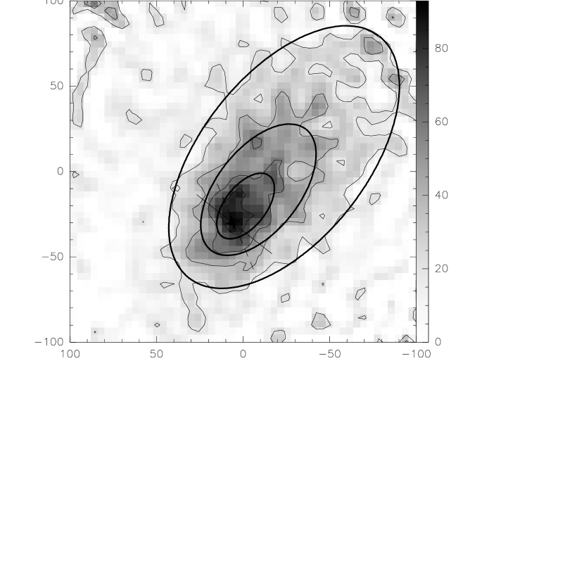
Figure 2: Iso-surface-brightness contours (thick solid lines) from a theoretically computed, lopsided, magnetized, self-gravitating figure of equilibrium compared with isophotal measurements of Ward-Thompson et al. (1999) of the submillimeter emission from heated dust grains in L1544. The short solid line and dashed line show the directions of predicted and measured field inferred from submillimeter-wave polarization observations (Ward-Thompson et al. 2000).

As an amusing sideshow, Figure 2 shows an overlay of one of our eccentrically displaced static models projected onto a map of thermal dust emission at 1.3 mm obtained by Ward-Thompson, Motte, & André (1999) for the prestellar molecular cloud core L1544. Apart from relatively minor fluctuations due to the cloud turbulence, the solid curves depicting the iso-surface-density contours of the theoretical model match well both the observed shapes and grey-scale of the dust isophotes.

Zeeman measurements of the magnetic-field component parallel to our line of sight toward L1544 have been made by Crutcher & Troland (2000), who obtain $B_{\parallel}=11\pm 2$ $\mu$G. For a highly flattened disk, which is reflection symmetric about the plane $z=0$, integration along the line of sight yields cancelling contributions of $B_{\varpi}$ and $B_{\varphi}$ to $B_{\parallel}$. The $z$-component of the magnetic field of our model core is given by

$$B_{z}={2\pi G^{1/2}\over\lambda}\Sigma.$$ (48)

We may now calculate the average value of $\Sigma$ within a radius $R$ as

$$\langle\Sigma\rangle={1\over\pi R^{2}}\oint d\varphi\int_{0}^{R}\Sigma\varpi\,d\varpi={\Theta a^{2}\over\pi\epsilon GR}={\lambda^{2}(\lambda^{2}+3)\over(\lambda^{4}-1)}{a^{2}\over\pi GR},$$ (49)

where we have made use of equations (4), (5), (15), (16) and (30). Therefore, the average value of $B_{z}$ within a radius $R$ is

$$\langle B_{z}\rangle={2\pi G^{1/2}\over\lambda}\langle\Sigma\rangle={\lambda(\lambda^{2}+3)\over(\lambda^{4}-1)}{2a^{2}\over G^{1/2}R}.$$ (50)

Notice the pleasant result that the above formulae do not involve $e$.

Since we model L1544 as a thin disk with elliptical iso-surface-density contours, its orientation in space is defined by three angles, two specifying the orientation of the disk plane, the third giving the position of the elliptical contours in this plane. We fix the first angle by assuming for simplicity that the major axis of the elliptical contours lies in the plane of the sky. The second angle $i$ is the inclination of the minor axis with respect to the plane of the sky ($i=0$ for a face-on disk) and can be adjusted to fit the observations. The third angle, specifying the ellipse’s orientation in the disk plane, is given as 38^∘ north through east by Ward-Thompson et al. (2000).

We choose the eccentricity $e$ and inclination $i$ by the following procedure. From Figure 2, we can estimate that a typical dust contour has a ratio of distances closest and farthest from the core center given in a model of nested confocal ellipses by

$${1-e\over 1+e}\approx 0.30\qquad\Rightarrow\qquad e\approx 0.54.$$ (51)

Similarly, we may estimate that these ellipses have an apparent minor-to-major axis-ratio of

$$(1-e^{2})^{1/2}\cos i\approx 0.54\qquad\Rightarrow\qquad\cos i\approx 0.64.$$ (52)

The resulting ellipses for three iso-surface-density contours, spaced in a geometric progression 1:2:4, are shown as solid curves in Figure 2.

Determination of $\cos i$ allows us to compute an expected $\langle B_{\parallel}\rangle$ = $\langle B_{z}\rangle\cos i$. Similarly, we obtain the expected hydrogen column density by multiplying $\langle\Sigma\rangle$ by $(\cos i)^{-1}$ for a slant path through an inclined sheet and by 0.7 for the mass fraction of H nuclei of mass $m_{H}$: $N_{H}=0.7\langle\Sigma\rangle/(m_{H}\cos i)$.

The sound speed for the 10 K gas in L1544 is $a=0.19$ km s^-1 (Tafalla et al. 1998). These authors give $\Delta V=0.22$ km s^-1 as the typical linewidth for their observations of C³⁴S in this region. For such a heavy molecule, turbulence is the main contributor to the linewidth, which allows us to estimate the mean square turbulent velocity along a typical direction (e.g., the line of sight) as $v_{t}^{2}=\Delta V^{2}/8\ln 2$. We easily compute that $v_{t}^{2}$ has only 24% the value of $a^{2}$. Assuming that it is possible to account for the “pressure” effects of such weak turbulence by adding the associated velocities in quadrature, $a^{2}+v_{t}^{2}$, we adopt an effective isothermal sound speed of $a=0.21$ km s^-1 for L1544.

The radius of the Arecibo telescope beam at the distance of L1544 is $R=0.06$ pc (Crutcher & Troland 2000). Ambipolar diffusion calculations by Nakano (1979), Lizano & Shu (1989), Basu & Mouschovias (1994) suggest that $\lambda\approx 2$ when the pivotal state is approached (see the summary of Li & Shu 1996). Putting together the numbers, $\cos i=0.64$, $R=0.06$ pc, $a=$ 0.21 km s^-1, and $\lambda=2$, we get $\langle B_{\parallel}\rangle=11$ $\mu G$, in excellent agreement with the Zeeman measurement of Crutcher & Troland (2000). These authors also deduce $N_{H}=1.8\times 10^{22}$ cm^-2 from their OH measurements, whereas we compute a hydrogen column density within the Arecibo beam of $N_{H}=1.4\times 10^{22}$ cm^-2. The slight level of disagreement is probably within the uncertainties in the calibration or calculation of the fractional abundance of OH in dark clouds (cf. Crutcher 1979, van Dishoeck & Black 1986, Flower 1990, Heiles et al. 1993).

Our ability to obtain good fits of much of the observational data concerning the prestellar core L1544 with a simple analytical model should be contrasted with other, more elaborate, efforts. Consider, for example, the axisymmetric numerical simulation of Ciolek & Basu (2000), who assumed a disk close to being edge-on ($\cos i\approx 0.3$ when $e$ is assumed to be 0) to reproduce the observed elongation, but who left unexplained the eccentric displacement of the cloud core’s center (very substantial for ellipses of eccentricity $e\approx 0.54$). The adoption of axisymmetric cores leads to another problem: Ciolek & Basu’s deprojected magnetic field is on average 3-4 times stronger than ours, values probably in conflict with Zeeman measurements of low-mass cloud cores. [See the comments of Crutcher & Troland (2000) concerning the need for magnetic fields in Taurus to be all nearly in the plane of the sky if conventional models are correct.] Natural elongation plus projection effects, as anticipated in the comments of Shu et al. (1999), allow us to model L1544 as a moderately supercritical cloud, with $\lambda\approx 2$, fully consistent with the theoretical expectations from ambipolar diffusion calculations, and in contrast with the value $\lambda\approx 8$ estimated by Crutcher & Troland (2000) from the measured values of $B_{\parallel}$ and $N_{H}$. In addition, if L1544 is a thin, intrinsically eccentric, disk seen moderately face-on, as implied by our model, then the extended inward motions observed by Tafalla et al. (1998; see also Williams et al. 1999) may be attributable to a (relatively fast) core-amplification mechanism that gathers gas (neutral and ionized) dynamically but subsonically along magnetic field lines on both sides of the cloud toward the disk’s midplane.

Finally, we show in Figure 2 the direction of the average magnetic field projected in the plane of the sky predicted by our model (thin solid line) and derived from submillimeter polarization observations of Ward-Thompson et al. (2000) (thin dashed line). Since we have assumed in our model that the major axis of iso-surface-density contours is in the plane of the sky, the predicted projection of the magnetic field is parallel to the cloud’s minor axis. The offset between the measured position angle of the magnetic field and the cloud’s minor axis might indicate some inclination of the cloud’s major axis with respect to the plane of the sky. The turbulent component of the magnetic field, not included in our model, may also contribute to the observed deviation.

4 Linear Perturbations of Axisymmetric Rotating SIDs

We now consider equilibrium configurations with internal motions: $D\neq 0$, $U(\varphi)\neq 0$. For comparison with the analysis of Paper I, we begin with a perturbative analysis of the equations of the problem valid for small deviation from axisymmetry.

For axisymmetric disks, $V_{m}=0$ for $m\geq 1$, and therefore equations (40) and (41) reduce to

$$S=S_{0}=1,\qquad V=V_{0}=-\ln 2.$$ (53)

Iso-surface-density contours are now circles. Substitution of these values into equation (33) and (34) yields $B=D$ and $U=0$. The dynamics of centrifugal balance is contained in the relationship (30) among the various constants of the problem:

$$K={\Theta a^{2}\over 2\pi\epsilon G}(1+D^{2}),$$ (54)

the same as equation (9) of Paper I. These axisymmetric SIDs are uniquely determined, in an irreducible sense, by a freely specifiable value of $D$. (Physically, we are also free, of course, to choose different scalings via $a$ and $\lambda$, with the latter determining $\epsilon$ and $\Theta$.)

Consider now small departures from these axisymmetric states characterized by a basic $M$-fold symmetry, with $M=1,2,3,\ldots$. Equations (40) and (41) give

$$S(\varphi)=1-MV_{M}\cos(M\varphi),$$ (55)

$$V(\varphi)=-\ln 2+V_{M}\cos(M\varphi).$$ (56)

Equation (55) shows that for small deviations from axisymmetric iso-surface-density contours are limaçons of Pascal (Dürer 1525).

As required by equation (32), $U(\varphi)$ must be expanded as a sine series,

$$U(\varphi)=U_{M}\sin(M\varphi).$$ (57)

To linear order, $B=D$ as in the axisymmetric case.

Substitution of the relations (55)-(57) into equations (34) and (32) of the governing set yields, after subtraction of the axisymmetric relations and linearizing,

$$M^{2}(1-D^{2})V_{M}-M(1+D^{2})V_{M}+DU_{M}=0,$$ (58)

$$-DV_{M}+U_{M}=DV_{M}.$$ (59)

Solutions are possible for arbitrary (infinitesimal) values of $V_{M}$ provided

$$U_{M}=2DV_{M},$$ (60)

and

$$M(1+D^{2})-M^{2}(1-D^{2})=2D^{2}.$$ (61)

Equation (61) is equivalent to equation (25) of Paper I and can be satisfied by $M=1$ for any rotation rate $D$ (including $D$ = 0). For $M>1$, we require special values of $D$:

$$D^{2}={M\over M+2}\qquad{\rm for}\qquad M=2,3,4,\dots$$ (62)

Notice the result that the required $D^{2}\rightarrow 1$ as $M\rightarrow\infty$.

For any given $D$, different values of $V_{M}\ll 1$ generate a continuum of linearized solutions. Without loss of generality, we can assume $V_{M}>0$, as the transformation $V_{M}\rightarrow-V_{M}$ is equivalent to a rotation of the equilibrium configuration by an angle $\pi/M$. (see discussion at the end of §2.2). To lowest order, the two components of the fluid velocity as given by equation (29) satisfy

$${u_{\varpi}\over\Theta^{1/2}a}=2DV_{M}\sin(M\varphi),$$ (63)

and

$${u_{\varphi}\over\Theta^{1/2}a}=D[1+V_{M}\cos(M\varphi)].$$ (64)

Therefore, for infinitesimal values of $V_{M}$ the flow describes a locus in the velocity plane $(u_{\varpi},u_{\varphi})$ which is an ellipse of axial ratio 2 centered on $(0,\Theta^{1/2}aD)$:

$$\left({u_{\varpi}\over 2\Theta^{1/2}a}\right)^{2}+\left({u_{\varphi}\over\Theta^{1/2}a}-D\right)^{2}=D^{2}V_{M}^{2}.$$ (65)

Notice that the axial ratios are a factor of $\sqrt{2}$ larger than the kinematic epicycles a collisionless body would generate upon being disturbed from a circular orbit in a disk that has a flat rotation curve (e.g., Binney & Tremaine 1987); the extra factor of $\sqrt{2}$ (and a non-precessing pattern with $M$ lobes) arises for a fluid disk because of the coherence enforced by the collective self-gravity of the perturbations.

As $V_{M}$ is increased, the flow must eventually try to cross the magnetosonic point, $u_{\varphi}=\Theta^{1/2}aD$, which is a singular point of equation (34). This transition cannot be followed without the introduction of shocks (see the analogous phenomena of spiral galactic shocks treated by Shu, Milione, & Roberts 1973). In the present context, smooth-flow solutions are possible only if $u_{\varphi}\leq\Theta^{1/2}a$ (entirely submagnetosonic flow, for $D<1$) or $u_{\varphi}\geq\Theta^{1/2}a$ (entirely supermagnetosonic flow, for $D>1$). When $D$ is close to 1, either slightly smaller or larger, the azimuthal velocity in the SID is very close to magnetosonic already in the axisymmetric case. Thus, the magnetosonic point is reached when deviations from axisymmetry are small, and the results of the linear analysis developed above can be applied. Equation (64) then gives the critical value of the coefficient $V_{M}$, in the linear regime, at which the flow tries to cross the magnetosonic point,

$$V_{M}^{\rm crit}\approx\pm\left(1-{1\over D}\right),$$ (66)

with the plus (minus) sign valid for $D>1$ ($D<1$).

5 Fully Nonlinear Models with Internal Motions

5.1 Numerical Method

In the general case, we solve the set of governing equations by iteration. For a given iterate when $S(\varphi)$ is known, we may regard equation (23) as an integral for $V(\varphi)$. Similarly, equations (32) and (28) constitute an ODE plus its starting condition for $U(\varphi)$. For general $\varphi$, equation (34) may now be solved as a first order ODE with the boundary condition equation (16) to obtain a new iterate for $S(\varphi)$. The procedure actually adopted substitutes a Fourier transform for a direct integration of equation (23), as described in §2.3.

(A) Fix the value of $D$ that one wants to study. Suppose we want to study a configuration with a basic $M$-fold symmetry, with $M=1,2,3,\dots$. Then we would begin with an initial guess for the Fourier coefficients $\{V_{m}\}_{m=1}^{\infty}$. We then compute

$$V(\varphi)=-\ln 2+\sum_{m=1}^{\infty}V_{m}\cos(mM\varphi),$$ (67)

and

$$S(\varphi)=1-M\sum_{m=1}^{\infty}mV_{m}\cos(mM\varphi).$$ (68)

(B) Compute the resulting value of $B$ from equation (33). Since the cycle need be taken only over $2\pi/M$ in $\varphi$, we have

$$B={MD\over 2\pi}\int_{0}^{2\pi/M}{d\varphi\over S(\varphi)}.$$ (69)

Integrate equation (32) for $U$ subject to the starting condition (28). Since $S$ has been forced to be a cosine series, $U$ is then automatically a sine series, i.e., we should automatically find $U(\varphi)$ to be $M$-periodic, with $U(2\pi/M)=0$.

(C) With $D$ fixed, and with $B$, $V(\varphi)$, $S(\varphi)$, and $U(\varphi)$, known in the form of the current iterates, solve equation (34) as a first order ODE for $S(\varphi)$, subject to the normalization condition (16). With this new iterate for $S(\varphi)$ compute the Fourier coefficients

$$V_{m}=-{1\over\pi m}\int_{0}^{2\pi/M}S(\varphi)\cos(mM\varphi)\,d\varphi\qquad{\rm for}\qquad m=1,2,\dots$$ (70)

Compare these coefficients with those from the previous iterate. If they are insufficiently precise, go back to step (A), after introducing, if necessary, a relaxation parameter to smooth between successive iterates for $V_{m}$.

5.2 Numerical Results

Results from our numerical integrations are illustrated in Figures 3–10. It is convenient to define a plane $(D^{2},S_{M})$, where $S_{M}=-MV_{M}$ is the first coefficient in the Fourier expansion of the function $S(\varphi)$, and can be considered an indicative measure of deviations from axial symmetry. Figure 3 shows the regions in the $(D^{2},S_{1})$ plane occupied by $M=1$ models with entirely submagnetosonic or entirely supermagnetosonic flow. At the upper limit of these two regions the flow attempts a magnetosonic transition at perisys (closest to the system center) in the former case and at aposys (farthest from the system center) in the latter case, as computed numerically with the method described in §5.1. The long-dashed line shows the same magnetosonic limit as given by equation (66) in the linear approximation $S_{1}\ll 1$. Notice that for $D=0$ the results of §3 show that $S_{1}^{\rm crit}=V_{1}^{\rm crit}=2$. Tick marks denote the values of $D^{2}$, as predicted by the linear analysis of Paper I and §4, where bifurcations occur with $M$-fold symmetry $(M\geq 2)$ from the axisymmetric sequence of SIDs that lie along the short dashed line.

Figure 4 shows submagnetosonic $M=1$ states for the case $D^{2}=0.1$ as $S_{1}$ progresses from the axisymmetric limit ($S_{1}=0$) to just before the magnetosonic transition ($S_{1}=1.39)$. Notice that flow velocities are largest at perisys because of the tendency to conserve specific angular momentum (not exact because the self-consistent gravitational field is nonaxisymmetric). As a consequence, the magnetosonic transition, when it arrives, is made at the minimum of the gravitational potential, as seen by a fluid element, when the base flow is submagnetosonic. Notice also that the iso-surface-density contours are quasi-elliptical with foci at the center of the system and with the major axes lying in the same direction as the elongation of the streamlines formed by connecting the flow arrows.

Figure 5 shows supermagnetosonic $M=1$ states for the case $D^{2}=4$ as $S_{1}$ progresses from the axisymmetric limit ($S_{1}=0$) to just before the magnetosonic transition ($S_{1}=1.08)$. Notice that flow velocities are smallest at aposys, again because of the (inexact) tendency to conserve specific angular momentum. As a consequence, the magnetosonic transition, when it arrives, is made at the maximum of the gravitational potential, as seen by a fluid element, when the base flow is supermagnetosonic. Notice also that the iso-surface-density contours are now elongated in the opposite sense to streamlines made by connecting the flow arrows.

We can explain the last difference between the submagnetosonic and supermagnetosonic cases (compare Figs. 3 and 4) by analogy with a forced harmonic oscillator, whose response is in phase or out of phase with the external sinusoidal forcing depending on whether the forcing frequency is lower or higher than the natural frequency. A similar effect evidently distinguishes the ability of fluid elements to respond in or out of phase to the nonaxisymmetric forcing of the collective gravitational potential depending on whether the flow occurs at submagnetosonic or supermagnetosonic speeds relative to the pattern speed (zero in the present case). This distinction could be developed as a powerful diagnostic of physical conditions in flattened cloud cores and massive protostellar disks, if both turn out to have lopsided shapes, because the former can generally be expected to have submagnetosonic rotation speeds; the latter, supermagnetosonic speeds.

Figure 6 shows additional examples of entirely submagnetosonic flow (for $D^{2}=0.5$) and entirely supermagnetosonic flow (for $D^{2}=1.5$) for $M=1$ SIDs, but now in the $(u_{\varpi},u_{\varphi})$ plane. Models are computed with different values of $S_{1}$ by the numerical method described in §5.1. For comparison, the corresponding flow solutions obtained with the linear analysis of §4 are also shown. Notice that the forced epicyclic motion by the nonaxisymmetric gravitational field about the gyrocenter marked with a cross (corresponding to circular motion of the axisymmetric model with the same value of $D^{2}$), approaches the magnetosonic transition (horizontal dashed line) in both cases along a tangent in the velocity-velocity plane. This behavior is peculiar to $M=1$ SIDs, and constitutes a topic to which we will return after discussing the $M>1$ cases.

Figure 7 shows the locus in the $D^{2}$–$|S_{M}|$ plane of sequences of equilibria with given $M$-fold symmetry, ranging from axisymmetric models (dashed line) to the points where the submagnetosonic flow acquires a magnetosonic transition (circles). We remind the reader that, unlike the $M=1$ case, bifurcation of $M>1$ sequences from the axisymmetric state occurs at discrete rather a continuum of values of $D^{2}$, given by $D^{2}=M/(M+2)$. Thus, $M=2,3,4,\dots$ sequences always begin submagnetosonically, $D^{2}<1$, at $S_{M}=0$, and terminate with a magnetosonic transition (circles) before the nonlinearity parameter $S_{M}$ can acquire very large values.

Figure 8 shows iso-surface-density contours and velocity vectors for $M=2$ equilibria ranging from the axisymmetric limit ($S_{2}=0$) to just before the magnetosonic transition ($S_{2}=0.229$). Notice the transformation from oval distortions at small $S_{2}$ (e.g., $S_{2}=0.1$) to dumbells at large $S_{2}$ (e.g., $S_{2}=0.2$). The latter shapes terminate at the magnetosonic transition ($S_{2}=0.229$), where the pinched neck of the dumbell develops a cusp and the streamlines are trying to change from circulation around a single center of attraction to circulation around what looks increasingly like two centers of attraction.

Figure 9 shows iso-surface-density contours and streamlines for models with $M$-fold symmetry, $M=2,3,4$ and 5, near the endpoints of the sequences shown in Figure 7. Finally, Figure 10 shows the velocity-velocity plots for the same four models. The solutions with $M>1$ in Figure 10 differ from those with $M=1$ in Figure 4 in that the magnetosonic transition for $M>1$ are made via the development of a cusp in both the iso-surface-density and velocity-velocity plots. We noted earlier that the magnetosnic transition is made for $M=1$ configurations with the $u_{\varpi}-u_{\varphi}$ locus becoming tangent to the critical curve.

5.3 Interpretation as Onset of Shocks

For gas flow in spiral galaxies, Shu et al. (1973) identified cusp formation in the velocity-velocity plane, as the onset of a shockwave with infinitesimal jumps, and we adopt a similar interpretation here. For trans-magnetosonic flow beyond the cusp solution (not shown in Figure 10 but see Shu et al. 1973), a smooth transition from submagnetosonic speeds to supermagnetosonic speeds is possible as the gas swings toward its closest approach to the center, but a smooth deceleration from supermagnetosonic speeds back to submagnetosonic speeds is not possible as this gas climbs outwards and catches up with slower moving material ahead of it. The transition to slower speeds is made instead via a sudden jump (a shockwave of finite strength). The shock jump introduces irreversibility to the flow pattern. Prior to the appearance of the shockwave, the flow can equally occur in the reverse direction as in the forward direction, and the streamlines close on themselves. After the appearance of a shockwave, time reversal is no longer possible, and the streamlines no longer close (see, e.g., the discussions of Kalnajs 1973 and Roberts & Shu 1973). Instead, angular momentum is removed from the gas (via gravitational torques when the patterns of density and gravitational potential show phase lags) and transferred outward in the disk, causing individual streamlines to spiral toward the center and increasing the central concentration of mass. The problem then becomes intrinsically time-dependent and cannot be followed by the steady-flow formulation given in the present paper.

We are uncertain why the magnetosonic transition in the case $M=1$ is not made via cusp-formation. It may be that in this special case, sufficient gravitational deceleration from supermagnetosonic to submagnetosonic speeds (rather than via pressure forces) can occur as to allow a smooth trans-magnetosonic flow to occur in a complete circuit. Unfortunately, we are unable to study this unprecedented behavior by the methods of the present paper because the numerical errors introduced by the truncated Fourier treatment of Poisson’s equation compromise our ability to judge true convergence in these difficult circumstances. In any case, it is hard to believe, even if smooth trans-magnetosonic solutions could be found for lopsided SIDs, that such solutions could be stable (in a time-dependent sense) to the creation of shockwaves by small departures from perfect 1-fold symmetry.

5.4 Circulation and Energy

It is interesting to ask whether the nonaxisymmetric bifurcation sequences studied in this paper represent merely adjacent equilibria, or also possible evolutionary tracks that might be accessed by secular evolution of a single system. To help answer this question, it is useful to compute the variation of four quantities along any sequence. The first quantity is the ratio $C\equiv{\cal C}/{\cal M}$ of the circulation $\cal C$ associated with a streamline to the mass $\cal M$ that it encloses. For scale-free equilibria, the value of $C$ is independent of the spatial location of the streamline used to perform the calculation. The second, third, and fourth quantities are the ratios $T\equiv{\cal T}/{\cal M}$, $P\equiv{\cal P}/{\cal M}$, and $W\equiv{\cal W}/{\cal M}$, respectively, of the kinetic energy $\cal T$, pressure work integral $\cal P$, and gravitational work integral $\cal W$ contained interior to any streamline, to the enclosed mass $\cal M$. The quantity $C$ is interesting because Kelvin’s circulation theorem (e.g., Shu 1992) combined with the equation of continuity states that $C$ is conserved in any time-dependent evolution of an ideal barotropic fluid. The quantities $T$, $P$, and $W$ are interesting because they must satisfy the following scalar virial theorem (per unit mass):

$$2T+\Theta P+\epsilon W=0.$$ (71)

Let $\varpi=\varpi_{0}(\varphi)$ define a streamline in the plane of the disk. The condition $\Psi={\rm const}$ in equation (24) gives immediately

$$\varpi_{0}(\varphi)\propto e^{W(\varphi)/D},$$ (72)

where the value of the proportionality constant is irrelevant for what follows [the reader should not confuse the function $W(\varphi)$ with $W\equiv{\cal W}/{\cal M}$]. The mass and kinetic energy contained interior to this streamline are

$${\cal M}=\int_{0}^{2\pi}\int_{0}^{\varpi_{0}(\varphi)}\Sigma\varpi d\varpi d\varphi,$$ (73)

$${\cal T}={1\over 2}\int_{0}^{2\pi}\int_{0}^{\varpi_{0}(\varphi)}\Sigma(u_{\varpi}^{2}+u_{\varphi}^{2})\varpi d\varpi d\varphi,$$ (74)

whereas the circulation and pressure and gravitational work integrals associated with this streamline are

$${\cal C}=\oint{\bf u}\cdot d{\bf l}=\int_{0}^{2\pi}\left(u_{\varpi}{d\varpi_{0}\over d\varphi}+u_{\varphi}\varpi_{0}\right)d\varphi,$$ (75)

$${\cal P}=-\int\int{\bf x}\cdot\nabla\Pi\,d^{2}x=-a^{2}\oint d\varphi\int_{0}^{\varpi_{0}(\varphi)}\varpi{\partial\Sigma\over\partial\varpi}\,\varpi d\varpi,$$ (76)

$${\cal W}=-\int\int\Sigma{\bf x}\cdot\nabla{\cal V}\,d^{2}x=-\oint d\varphi\int_{0}^{\varpi_{0}(\varphi)}\varpi{\partial{\cal V}\over\partial\varpi}\Sigma\,\varpi d\varpi.$$ (77)

Notice that the quantity $\cal P$ equals twice the thermal energy minus a surface term only if we perform an integration by parts, which we do not do here (cf. §3.2 in Paper I).

If we introduce the nondimensional variables defined in §2.2, these expressions become

$${\cal M}=KI_{1},\qquad{\cal T}={1\over 2}K\Theta a^{2}I_{2},$$ (78)

$${\cal C}={\Theta^{1/2}a\over D}I_{2},\qquad{\cal P}=a^{2}KI_{1},\qquad\qquad{\cal W}=-2\pi GK^{2}I_{1},$$ (79)

where we have used equation (22) to evaluate $\varpi\partial{\cal V}/\partial\varpi$ as $2\pi GK$, and where

$$I_{1}\equiv\int_{0}^{2\pi}S\varpi_{0}\;d\varphi,\qquad I_{2}\equiv\int_{0}^{2\pi}{U^{2}+D^{2}\over S}\varpi_{0}\;d\varphi.$$ (80)

Multiplying equation (32) by $\varpi_{0}(\varphi)$ defined by equation (72) and integrating over a complete cycle, we obtain

$${I_{2}\over I_{1}}=DB.$$ (81)

Therefore,

$$C\equiv{{\cal C}\over{\cal M}}={2\pi\epsilon G\over\Theta^{1/2}a}\left({B\over 1+DB}\right),$$ (82)

and

$$P\equiv{{\cal P}\over{\cal M}}=a^{2},\qquad T\equiv{{\cal T}\over{\cal M}}={\Theta a^{2}\over 2}DB,\qquad W\equiv{{\cal W}\over{\cal M}}=-{\Theta a^{2}\over\epsilon}(1+DB),$$ (83)

where we have used equation (30) to eliminate $K$. With the expressions (83), the scalar virial theorem (71) is satisfied identically.

Since $M=1$ equilibria exist as a densely populated set of points in the $D^{2}$–$|S_{1}|$ plane, it is clear that we can choose many sequences for them that have constant values for $C$. For fixed $\lambda$ (field freezing) and $a$ (isothermal systems), $C$ is constant along curves of constant $B/(1+DB)$ = $D_{0}/(1+D_{0}^{2})$, where $D_{0}$ is the axisymmetric value of $D$. Thus, on such a sequence,

$$BD={D_{0}D\over 1+D_{0}(D_{0}-D)}.$$ (84)

The dotted curves in Figure 3 show such loci for two representative sequences in the $D^{2}$–$|S_{1}|$ plane: one submagnetosonic, the other supermagnetosonic. At the beginning and end of the supermagnetosonic sequence displayed in Figure 3, $D_{0}^{2}=1.50$ and $D^{2}=1.84$. Hence, $BD$ varies from 1.50 at the beginning to 1.98 at the end, and $-W\propto(1+BD)$ therefore increases by about 19% from beginning to end. In other words, rapidly rotating, self-gravitating SIDs with diplaced centers are more gravitationally bound than their axisymmetric counterparts. In the presence of dissipative agents that lower the energy while preserving the circulation, such disks will secularly tend toward greater asymmetric elongation (see Fig. 5). More gravitational energy is released when distorted streamlines bring matter closer to the center than is expended when the same streamlines take the matter farther from the center, conserving circulation. This exciting result deserves further exploration both theoretically and observationally for systems other than the full singular isothermal disk.

At the beginning and end of the submagnetosonic sequence displayed in Figure 3, $D_{0}^{2}=0.60$ and $D^{2}=0.35$. Hence, $BD$ varies from 0.60 at the beginning to 0.40 at the end, and $-W\propto(1+BD)$ therefore decreases by about 12% from beginning to end. This variation is not very much considering how fast this sequence rotates relative to realistic cloud cores. Nevertheless, the formal decrease of $-W$ as one leaves the axisymmetric state implies that submagnetosonic systems require some input of energy to make them less round. Exceptions are sequences that branch from smaller values of $D_{0}^{2}$, which have smaller variations of $-W$. In particular, long spindles have no binding energy disadvantage whatsoever relative to axisymmetric disks for the nonrotating sequence shown in Figure 1, because here $-W\propto(1+BD)=1$, a constant. In this regard, it may be significant that observed cores that are significantly lopsided (see Fig. 2) typically rotate quite slowly.

The story is more ambiguous for $M>1$ equilibria. Here, for given $M$, the stationary states occupy one-dimensional curves in the $D^{2}$–$|S_{M}|$ plane; therefore, we have no control over how $C$ and $-W$ vary along any sequence. Plotted in Figure 11 are the values of $C$ and $-W$ as we vary $S_{M}$ along the sequences for $M=$ 2, 3, 4, 5. Amazingly, the normalized circulation $C$ is nearly, but not exactly, constant on each sequence, varying by no more than 1% in all cases. Given the small values of $S_{M}$ for which solutions exist and the relatively small variation of $D$ along each sequence, this result is not surprising, because $B$ and $DB$ differ from their values for axisymmetric SIDs by terms ${\cal O}(S_{M}^{2})$. Although in principle secular evolution along any $M>1$ sequence would require a slight redistribution of circulation with mass, the amount required is truly slight, and one could imagine that mechanisms might exist that can effect a slow transformation along the sequence toward more nonaxisymmetric states. In principle, such evolution would seem to favor the formation of $M$ = 2, 3, 4, 5, …buds, depending on the rate of rotation present in the underlying flow. However, before 2, 3, 4, 5, …independently orbiting bodies can form by such a “fission” process, this sequence of events would terminate in shockwaves, and the resultant transfer of angular momentum (or circulation) outward and mass inward would stabilize the system against actual successful fission.

The non-constancy of $C$ along sequences of equilibria with fixed $M$ is reminescent of the change of equatorial circulation along the Jacobi sequence of incompressible ellipsoids at fixed $J$ and $M$ (Lynden-Bell 1965). A frictionless body is incapable of evolving along the Jacobi sequence, and a Maclaurin spheroid cannot fall into a Jacobi ellipsoid, in agreement with the known stability of the frictionless spheroid at the bifurcation point . In practice, for gaseous systems, a more practical difficulty mitigates against even beginning the secular paths of evolution described in the previous paragraphs for the submagnetosonic cases. The nonaxisymmetric SIDs with $M=2,3,4,5$ depicted in Figures 8 and 9 are all rotating too slowly to be stable against “inside-out” collapse of the type studied for their axisymmetric counterpart by Li & Shu (1997). This dynamical instability would formally overwhelm any secular evolution along the lines described above. (Supermagnetosonic $M=1$ configurations rotate quickly enough to be stable against “inside-out” dynamical collapse, and a secular transformation to the more elongated and eccentrically displaced states of Fig. 5 are realistic theoretical possibilities.) We plan to study the dynamical collapse and fragmentation properties of nonaxisymmetric, submagnetosonic SIDs with general $M$-fold symmetry in a future paper. In another treatment, we shall also discuss the question whether configurations with strict $M>1$ symmetry are formally (secularly) unstable also to perturbations of $M=1$ periodicity (i.e., to additional “lopsided” bifurcations). But, for the present, we merely remark that the practical attainment of any of the nonaxisymmetric pivotal states depicted, say, in Figure 8 probably occurs, not along a sequence where each member has already achieved a (nearly) singular value of surface density at the origin $\varpi=0$, but along a line of evolution (perhaps by ambipolar diffusion) where the growing central concentration of matter occurs without the a priori assumption of axial symmetry (e.g., nonaxisymmetric generalizations of the calculations of Basu & Mouschovias 1994).

6 Summary and Discusssion

In this paper we have shown that prestellar molecular cloud cores modeled in their pivotal state just before the onset of gravitational collapse (protostar formation and envelope infall) as magnetized singular isothermal disks need not be axisymmetric. The most impressive distortions are those that make slowly rotating circular cloud cores lopsided ($M=1$ asymmetry). Although slowly rotating, lopsided cloud cores have a slight disadvantage relative to their axisymmetric counterparts from an energetic point of view, such elliptical configurations do seem to appear in nature (see Fig. 2).

More intriguingly, elongated, eccentrically displaced, supermagnetosonically rotating SIDs (that are stable to overall graviational collapse) are preferred to their axisymmetric counterparts if the excess binding energy of the latter can be radiated away without changing the circulation of the streamlines. If the mass of the circumstellar disk of a very young protostar is a large fraction of the mass of the system, it might be possible to find such $M=1$ distortions of actual objects by future ALMA observations. If such disks have (perturbed) flat rotation curves, we predict (see Fig. 5) that the mm-wave isotphotes should be elongated perpendicular to an eccentrically displaced central star and also perpendicular to the eccentric shape of the streamlines (as might be deducible from isovelocity plots common for investigations of spiral and barred galaxies).

Bifurcations into sequences with $M=2$, 3, 4, 5, and higher symmetry require rotation rates considerably larger ($>0.7$ times the magnetosonic speeds) than is typically measured for observed molecular cloud cores (e.g., Goodman et al. 1993). Although seemingly more promising for binary and multiple star-formation, the models with $M=2$, 3, 4, 5, … symmetries all terminate in shockwaves before their separate lobes can succeed in forming anything that resembles separate bodies (see Fig. 8). For these configurations to exist at all, the basic rotation rate has to be fairly close to magnetosonic. It is then not possible for the nonaxial symmetry to become sufficiently pronounced as to turn streamlines that circulate around a single center to streamlines that circulate around multiple centers (as is needed to form multiple stars), without the distortions causing supermagnetosonically flowing gas to slam into submagnetosonically flowing gas. The resultant shockwaves then increase the central concentration in such a fashion as to suppress the tendency toward fission.

We have managed to gain the above understanding semi-analytically only because of the mathematical simplicity of isopedically magnetized SIDs. The same understanding probably underlies similar findings from numerical simulations of the fission process that inevitably end with the creation of shockwaves before the actual production of two or more separately gravitating bodies (Tohline 2000, personal communication). This negative result, combined with the analysis of the spiral instabilities that afflict the more rapidly rotating, self-gravitating, disks into which more slowly rotating, cloud cores collapse (also modeled here as SIDs), is cause for pessimism that a successful mechanism of binary and multiple star-formation can be found by either the fission or the fragmentation process acting in the aftermath of the gravitational collapse of marginally supercritical clouds during the stages when field freezing provides a good dynamical assumption.

It might be argued that our analysis also assumed smooth starting conditions, and that therefore, turbulence might be the more important missing ingredient. However, the low-mass cloud cores in the Taurus molecular cloud that gives rise to many binaries and multiple-star systems composed of sunlike stars are notoriously quiet, with turbulent velocities that are only a fraction of the thermal sound speed (e.g., Fuller & Myers 1992). Such levels of turbulence are well below those that appear necessary to induce “turbulent fragmentation” in the numerical simulations of Klein et al. (2000). Interstellar turbulence is undoubtedly an important process at the larger scales that characterize the fractal structures of giant molecular clouds (see, e.g., Allen & Shu 2000), but it probably plays only a relatively minor role in the simplest case of isolated or distributed star-formation that we see in clouds like those in the Taurus-Auriga region, which has, as we mentioned earlier, more than its share of cosmic binaries.

In contrast, we know that the dimensionless mass-to-flux ratio $\lambda$ had to increase from values typically $\sim 2$ in cloud cores to values in excess of 5000 in formed stars (Li & Shu 1997). Massive loss of magnetic flux must have occurred at some stage of the gravitational collapse of molecular cloud cores to form stars. Moreover, this loss must take place at some point at a dynamical rate, or even faster, since the collapse process from pivotal molecular cloud cores is itself dynamical. It is believed that dynamical loss of magnetic fields from cosmic gases occurs only when the volume density exceeds $\sim 10^{11}$ H₂ molecules cm^-3 (e.g., Nakano & Umebayashi 1986a,b; Desch & Mouschovias 2000). It might be thought that cloud cores have to collapse to fairly small linear dimensions before the volume density reaches such high values, and therefore, that only close binaries can be explained by such a process, but not wide binaries (McKee 2000, personal communication). However, this impression is gained by experience with axisymmetric collapse. Once the restrictive assumption of perfect axial symmetry is removed, we gain the possibility that some dimensions may shrink faster than others (e.g., Lin, Mestel, & Shu 1965), and densities as high as $10^{11}$ cm^-3 might be reached while only one or two dimensions are relatively small, and while the third is still large enough to accomodate the (generally eccentric) orbits of wide binaries.

We close with the following analogies. The basic problem with trapped magnetic fields is that they compress like relativistic gases (i.e., their stresses accumulate as the 4/3 power increase of the density in 3-D compression). Such gases have critical masses [e.g., the Chandrasekhar limit in the theory of white dwarfs, or the magnetic critical mass of equation (2)] which prevent their self-gravitating collections from suffering indefinite compression, no matter how high is the surface pressure, if the object masses lie below the critical values. Moreover, while marginally supercritical objects might collapse to more compact objects (e.g., white dwarfs into neutron stars, or cloud cores into stars), a single such object cannot be expected to naturally fragment into multiple bodies (e.g., a single white dwarf with mass slightly bigger than the Chandrasekhar limit into a pair of neutron stars).

In order for fragmentation to occur, it might be necessary for the fluid to decouple rapidly from its source of relativistic stress. For example, the universe as a whole always has many thermal Jeans masses. Yet in conventional big-bang theory, this attribute did not do the universe any good in the problem of making gravitationally bound subunits, as long as the universe was tightly coupled to a relativistic (photon) field. Only after the matter field had decoupled from the radiation field in the recombination era, did the many fluctuations above the Jeans scale have a chance to produce gravitational “fragments.” It is our contention that this second analogy points toward where one should search for a viable theory of the origin of binary and multiple stars from the gravitational collapse of magnetized molecular cloud cores.

Appendix A Appendix

Given the definition

$$L_{m}\equiv{1\over 2\pi}\oint\ln(1-\cos\varphi)\cos(m\varphi)\,d\varphi={1\over\pi}\int_{0}^{\pi}\ln(1-\cos\varphi)\cos(m\varphi)\,d\varphi,$$ (A1)

where $m$ is an integer (positive or negative), we show that

$$L_{m}=\left\{\begin{array}[]{ll}-\ln 2&\mbox{if $m=0$},\\ -1/|m|&\mbox{if $|m|\geq 1$}.\end{array}\right.$$ (A2)

(1) For $m=0$,

$$L_{0}={1\over 2\pi}\oint\ln(1-\cos\varphi)\,d\varphi={1\over\pi}\int_{0}^{\pi}\ln(1-\cos\varphi)\,d\varphi$$ (A3)

Successive transformations $\varphi\rightarrow-\varphi$ and $\varphi\rightarrow\varphi+\pi$ demonstrate

$$L_{0}={1\over\pi}\int_{-\pi}^{0}\ln(1-\cos\varphi)\,d\varphi={1\over\pi}\int_{0}^{\pi}\ln(1+\cos\varphi)\,d\varphi,$$ (A4)

which is just a statement that $\cos\varphi$ is odd relative to the midpoint of the interval $(0,\pi)$. If we add equations (A3) and (A4), we get

$$2L_{0}={1\over\pi}\int_{0}^{\pi}\ln(1-\cos^{2}\varphi)\,d\varphi={1\over\pi}\int_{0}^{\pi}\ln(\sin^{2}\varphi)\,d\varphi.$$ (A5)

Rewrite $\sin^{2}\varphi=(1/2)(1-\cos\chi)$ where $\chi\equiv 2\varphi$; then

$$2L_{0}=-\ln 2+{1\over 2\pi}\int_{0}^{2\pi}\ln(1-\cos\chi)\,d\chi.$$ (A6)

But the last integral is another expression for $L_{0}$ (see eq. [A3]); thus, $L_{0}=-\ln 2$. (QED)

(2) Integrate equation (A1) once by parts to obtain

$$mL_{m}=-{1\over 2\pi}\int_{-\pi}^{+\pi}{\sin(m\varphi)\sin\varphi\,d\varphi\over 1-\cos\varphi},$$ (A7)

Multiply and divide the integrand by $1+\cos\varphi$ and write $1-\cos^{2}\varphi$ as $\sin^{2}\varphi$. Thereby obtain

$$mL_{m}=-(I_{m}+J_{m}),$$ (A8)

where

$$I_{m}\equiv{1\over 2\pi}\int_{-\pi}^{+\pi}{\sin(m\varphi)\,d\varphi\over\sin\varphi},$$ (A9)

$$J_{m}\equiv{1\over 2\pi}\int_{-\pi}^{+\pi}{\sin(m\varphi)\cos\varphi\,d\varphi\over\sin\varphi}.$$ (A10)

We easily find

$$I_{1}=1\qquad{\rm and}\qquad J_{1}=0.$$ (A11)

For $m>1$, write

$$\sin(m\varphi)=\sin\varphi\cos[(m-1)\varphi]+\cos\varphi\sin[(m-1)\varphi].$$ (A12)

Equation (A9) then yields

$$I_{m}=J_{m-1},$$ (A13)

whereas equation (A10) becomes

$$J_{m}={1\over 2\pi}\int_{-\pi}^{+\pi}\left[\cos[(m-1)\varphi]\cos\varphi+{\cos^{2}\varphi\sin[(m-1)\varphi]\over\sin\varphi}\right]\,d\varphi.$$ (A14)

Write $\cos^{2}\varphi$ in the second term as $1-\sin^{2}\varphi$. Note that the $-\sin^{2}\varphi$ term combines with the other term in the integrand to form $\cos(m\varphi)$, which integrates to zero for $m>1$. Thus, obtain

$$J_{m}={1\over 2\pi}\int_{-\pi}^{+\pi}{\sin[(m-1)\varphi]\,d\varphi\over\sin\varphi}=I_{m-1}.$$ (A15)

Collecting results, we get

$$I_{m}+J_{m}=I_{m-1}+J_{m-1}=\dots=I_{1}+J_{1}=1\qquad{\rm for}\qquad m\geq 1.$$ (A16)

Since $L_{m}$ is an even function of $m$, equation (A8) now implies $L_{m}=-1/|m|$ for $|m|\geq 1$. (QED)

Figure 1: Iso-surface-density contours for static SIDs are perfect ellipses with eccentricity $e$. For $e=0$ the SID is an axisymmetric disk with surface density $\propto\varpi^{-1}$, for $e=1$ the SID degenerates in a semi-infinite filament of constant linear mass density.

Figure 3: The loci (solid curves) in the $(D^{2},|S_{1}|)$ plane of critical flow solutions for $M=1$ approaching magnetosonic speed starting from entirely submagnetosonic ($D<1$) or entirely supermagnetosonic flow ($D>1$). The horizontal short-dashed line shows the locus of axisymmetric models. The long-dashed curves shows the limit of magnetosonic models as given by equation (66) in the linear approximation $S_{1}\ll 1$. The dotted curves show a submagnetosonic and a supermagnetosonic sequence, each of which maintains a constant ratio $C$ of circulation $\cal C$ to enclosed mass $\cal M$ (see §5.4). Tickmarks pointing downward from the horizontal dashed line denote the values of $D^{2}$ where distortions with $M$-fold symmetry can occur, with $M>1$, as predicted by the linear analysis of Paper I and §4.

Figure 4: Sequence of equilibria with $M=1$ and $D^{2}=0.1$ for $S_{1}=0$ (axisymmetric case), 0.3, 0.6 and 1.39 (magnetosonic flow). Thick lines correspond to iso-surface-density contours logarithmically spaced. Streamlines are outlined by vectors of length proportional to the modulus of velocity, drawn to scale in the four panels. Equation (29) shows that the flow velocities depend, in magnitude and direction, only on the azimuthal angle $\varphi$ and not on the distance $\varpi$ (for given $\varphi$) from the center of the mass distribution. In particular, the gas velocities at perisys (or aposys) are all the same independent of the size of the streamline. In the last panel, the thin dotted line indicates the locus of magnetosonic velocity reached at perisys.

Figure 5: Sequence of equilibria with $M=1$ and $D^{2}=4$ for $S_{1}=0$ (axisymmetric case), 0.4, 0.8 and 1.08 (magnetosonic flow). Vectors and lines are as in Fig. 4.

Figure 6: Two examples of entirely submagnetosonic flow ($D^{2}=0.5$) and entirely supermagnetosonic flow ($D^{2}=1.5$) in the velocity-velocity plane, for $M=1$. In each panel, the axisymmetric solutions is marked by a cross. The two inner solid curves are obtained with $S_{1}=0.1$ and $0.2$, whereas the dotted curves show the corresponding linearized solutions. The outermost solid curve, obtained with $S_{1}=0.3235$ for $D^{2}=0.5$ and $S_{1}=0.2326$ for $D^{2}=1.5$, shows the approach to azymuthal magnetosonic flow (dashed line) defined by the condition $u_{\varphi}=\Theta^{1/2}a$.

Figure 7: Locus in the $D^{2}$–$|S_{M}|$ plane of sequences of equilibria with given $M$-fold symmetry. The dashed line indicates the locus of axisymmetric equilibria. Tickmarks denote the values of $D^{2}$ where distortions with $M$-fold symmetry can occur, as predicted by the linear analysis of Paper I and §4. Circles indicate the points where the sequences terminate because of the occurrence of shocks.

Figure 8: Sequence of equilibria with $M=2$, for $S_{2}=0$ (axisymmetric case), 0.1, 0.2 and 0.229 (magnetosonic flow). Vectors and lines are as in Fig. 4.

Figure 9: Iso-surface-density contours (thick lines) and streamlines (thin lines) for models with $M$-fold symmetry $M=2,3,4$ and 5 at the point of shock formation. Iso-surface-density contours develop cusps where the azymuthal flow velocity reaches the magnetosonic value.

Figure 10: Velocity-velocity plots for the four models shown in Fig. 8.

Figure 11: Values of $C$ and and $-W$, in units of $2\pi\epsilon G/\Theta^{1/2}a$ and $\Theta a^{2}/\epsilon$, respectively, as functions of $|S_{M}|$ along the sequences for $M=2$, 3, 4 and 5 shown in Figure 7. Circles indicate the points where the sequences terminate because of the occurrence of shocks.

References

- (1) Allen, A., & Shu, F. H. 2000, ApJ, 536, 368
- (2) Basu, S., & Mouschovias, T. Ch. 1994, ApJ, 432, 720
- (3) Baureis, P., Ebert, R., & Schmitz, F. 1989, A&A, 225, 405
- (4) Binney, J., & Tremaine, S. 1987, Galactic Dynamics, (Princeton: Princeton University Press)
- (5) Bonnor, W. B. 1955, MNRAS 115, 310
- (6) Boss, A. P. 1993, ApJ 410, 157
- (7) Brandner, W., Alcala, J. M., Kunkel, M., Moneti, A., & Zinnecker, H. 1996, A&A 307, 121
- (8) Burkert, A., Bate, M. R., & Bodenheimer P. 1997, MNRAS 289, 497
- (9) Cartan, H. 1928, in Proc. International Math. Congress, Vol. 2, p. 2 (Toronto: University of Toronto Press)
- (10) Chandrasekhar, S. 1969, Ellipsoidal Figures of Equilibrium (Yale University Press: New Haven)
- (11) Ciolek, G. E., & Basu, S. 2000, ApJ, 529, 925
- (12) Crutcher, R. M. 1979, ApJ 234, 881
- (13) Crutcher, R. M. 1999, ApJ 520, 706
- (14) Crutcher, R. M., & Troland, T. H. 2000, ApJ, 537, L139
- (15) Darwin, G. H. 1906, Phil. Trans. R. Soc. (London), 206, 161
- (16) Darwin, G. H. 1909, in Darwin and Modern Science, ed. A. C. Seward, (Cambridge Univ. Press), p. 543
- (17) Desch, S. J., & Mouschovias, T. Ch. 2000, ApJ, submitted
- (18) Dürer, A. 1525, Underweysung der Messung mit dem Zirckel und Richtscheyt, in Linien, Ebnen und Ganzen Corporen (Nuremberg)
- (19) Durisen, R. H., Gingold, R. A., Tohline, J. E., & Boss, A. P. 1986, ApJ 305, 281
- (20) Ebert, R. 1955, Z. Astrophys., 37, 217
- (21) Evans, N. J., Rawlings, J. M. C., Shirley, Y. L., & Mundy, L. G. 2000, in preparation
- (22) Flower, D. 1990, Molecular Collisions in the Interstellar Medium (Cambridge Univ. Press)
- (23) Fuller, G. A., & Myers, P. C. 1992, ApJ, 384, 523
- (24) Ghez, A. M., Neugebauer, G., & Matthews, K. 1993, AJ, 106, 2005
- (25) Goodman, A. A., Benson, P. J., Fuller, G. A., & Myers, P. C. 1993, ApJ, 406, 528
- (26) Gradshteyn, I. S., Ryzhik, I. M. 1965, Tables of Integrals, Series and Products, (Academic Press: New York)
- (27) Heiles, C., Goodman, A. A., McKee, C. F., & Zweibel, E. G. 1993, in Protstars and Planets III, ed. E. H. Levy & J. I. Lunine (Tucson: Univ. Arizona Press), 279
- (28) Hayashi, C., Narita, S., & Miyama, S. M. 1982, Prog. Theor. Phys., 68, 1949
- (29) Hoyle, F. 1953, ApJ 118, 513
- (30) Hunter, C. 1962, ApJ 136, 594
- (31) Jacobi, C. G. J. 1834, Poggendorff Annalen der Physik und Chemie, 33, 229
- (32) James, R. A. 1964, ApJ, 140, 552
- (33) Jeans, J. H. 1902, Phil. Trans. R. Soc. (London), 199, 49
- (34) Kalnajs, A. J. 1973, Proc. Astron. Soc. Australia, 2, 174
- (35) Klein, R. I., Fisher, R. T., McKee, C. F. 2000, in Proc. IAU 200, Formation of Binary Stars, ed. H. Zinnecker & R. Mathieu, in press
- (36) Larson, R. B. 1969, MNRAS, 145, 271
- (37) Laughlin, G., & Bodenheimer, P. 1994, ApJ, 436, 335
- (38) Laughlin, G., Korchagin, V. I., & Adams, F. C. 1998, ApJ, 504, 945
- (39) Layzer, D. 1964, ARA&A, 2, 341
- (40) Leinert, C., Zinnecker, H., Weitzel, N., Christou, J., Ridgway, S. T., Jameson, R., Haas, M., & Lenzen, R. 1993, A&A, 278, 129
- (41) Liapounoff, A. 1905, Mémoires de l’Académie Impériale des Sciences de St. Petersbourg, series 8, Classe Physico-Mathématique, 17, n. 3, p. 1
- (42) Li, Z.-Y., & Shu, F. H. 1996, ApJ, 472, 211
- (43) Li, Z.-Y., & Shu, F. H. 1997, ApJ 475, 237
- (44) Lin, C. C., Mestel, L., & Shu, F. H. 1965, ApJ, 142, 143
- (45) Lizano, S., & Shu, F. H. 1989, ApJ, 342, 834
- (46) Lynden-Bell, D. 1965, ApJ, 142, 1648
- (47) Lynden-Bell, D., & Katz, J. 1981, Proc. R. Soc. Lond. A, 378, 179
- (48) Looney, L. W., Mundy, L. G., & Welch, W. J. 1997, ApJ, 484, L157
- (49) Mathieu, R. D. 1994, ARA&A, 32, 465
- (50) Maclaurin, C. 1742, A Treatise on Fluxions
- (51) Medvedev, M. V., & Narayan, R. 2000, ApJ, 541, 579
- (52) Mestel, L., & Spitzer, L. Jr. 1956, MNRAS, 116, 503
- (53) Mestel, L. 1965a, Quart. J. Roy. Astron. Soc. 6, 161
- (54) Mestel, L. 1965b, Quart. J. Roy. Astron. Soc. 6, 265
- (55) Mestel, L., 1985, in Protostars & Planets II, eds. D. C. Black & M. S. Matthews (Tucson: University of Arizona Press), p. 320
- (56) Meyer, C. O. 1842, J. f. reine und angew, Math. (Crelle), 24, 44
- (57) Myers, P. C., & Benson, P. J 1983, ApJ 266, 309
- (58) Nakano, T. 1979, PASJ 31, 697
- (59) Nakano, T., & Umebayashi, T. 1986a, MNRAS, 218, 663
- (60) Nakano, T., & Umebayashi, T. 1986b, MNRAS, 221, 319
- (61) Ostriker, J. P., & Bodenheimer, P. 1973, ApJ, 180, 171
- (62) Ostriker, J. P., & Mark, J. W.-K. 1968, ApJ, 151, 1075
- (63) Poincaré, H. 1885, Acta Mathematica, 7, 259
- (64) Pickett, B. K., Cassen, P., Durisen, R. H., & Link, R. 1998 ApJ 504, 468 quoted as 1999
- (65) Shu, F. 1992, The Physics of Astrophysics, Vol. II: Gas Dynamics (Mill Valley, CA: University Science Books)
- (66) Shu, F. 1977, ApJ, 214, 488
- (67) Shu, F. H., Adams, F. C., & Lizano, S. 1987, ARA&A, 25, 23
- (68) Shu, F. H., Laughlin, G., Lizano, S., & Galli, D. 2000, ApJ, 535, 190 (Paper I)
- (69) Shu, F. H., Li, Z.-Y. 1997, ApJ, 475, 251
- (70) Shu, F. H., Milione, V., & Roberts, W. W. 1973, ApJ, 183, 819
- (71) Shu, F. H., Allen, A., Shang, H., Ostriker, E. C., & Li, Z.-Y. 1999 in The Origin of Stars and Planetary Systems, eds. C. J. Lada & N. D. Kylafis, Kluwer Academic Publishers, p. 193
- (72) Simon, M., Ghez, A. M., Leinert, Ch., Cassar, L., Chen, W. P., Howell, R. R., Jameson, R. F., Matthews, K., Neugebauer, G., & Richichi, A. 1995, ApJ, 443, 625
- (73) Syer, D., & Tremaine, S. 1996, MNRAS, 282, 223
- (74) Tafalla, M., Mardones, D., Myers, P. C., Caselli, P., Bachiller, R., & Benson, P. J. 1998, ApJ 504, 900
- (75) Terebey, S., Shu, F. H., & Cassen, P. 1984, ApJ 286, 529
- (76) Todhunter, I. 1873 History of the Mathematical Theories of Attraction and the Figure of the Earth (Constable: London)
- (77) Tohline, J. 1982, Fund. Cosm. Phys., 8, 1
- (78) Tomley, L., Steiman-Cameron, T. Y., & Cassen, P. 1994, ApJ 422 850
- (79) Toomre, A. 1977, ARAA, 15, 437
- Toomre (82) Toomre, A. 1982, ApJ, 259, 535
- (81) Truelove, J. K., Klein, R. I., McKee, C. F., Holliman, J. H. II., Howell, L. H., Greenough, J. A., & Woods, D. T. 1998, ApJ, 295, 821
- (82) van Dishoeck, E. F., & Black, J. H. 1986, Ap. J. Suppl. 62, 109
- (83) Ward-Thompson, D., Scott, P. F., Hills, R. E., & André, P. 1994, MNRAS, 268, 276
- (84) Ward-Thompson, D., Motte, F., & André, P. 1999, MNRAS, 305, 143
- (85) Ward-Thompson, D., Kirk, J. M., Crutcher, R. M., Greaves, J. S., Holland, W. S., & André, P. 2000, ApJL, 537, L135
- (86) Williams, J. P., Myers, P. C., Wilner, D. J., Di Francesco, J. 1999, ApJ 513, L61
- (87) Zucconi, A., & Walmsley, M. C. 2000, in preparation