Abstract

The effect of shear on the growth of large scale magnetic fields in helical turbulence is investigated. The resulting large-scale magnetic field is also helical and continues to evolve, after saturation of the small scale field, on a slow resistive time scale. This is a consequence of magnetic helicity conservation. Because of shear, the time scale needed to reach an equipartition-strength large scale field is shortened proportionally to the ratio of the resulting toroidal to poloidal large scale fields.

1 Introduction

Magnetic helicity is conserved in ideal MHD. In non-ideal situations, when magnetic diffusivity is non-vanishing, it can only evolve on a long time scale governed by microscopic magnetic diffusivity. This is true in periodic or unbounded systems or in systems with perfectly conducting boundaries, where no flux of magnetic helicity through the boundaries is allowed. In systems with open boundaries, magnetic helicity can leak out and the evolution in time can thus be different.

The importance of magnetic helicity conservation for the evolution of large-scale magnetic fields in astrophysics has been recently discussed (Blackman & Field 2000, Brandenburg 2000, Brandenburg & Subramanian 2000, Kleeorin et al. 2000). Large-scale, helical magnetic fields where the outer scale of turbulent motions is much smaller than the scale of these fields, are observed in stars and galaxies. For the Sun significant amounts of magnetic helicity are observed at the solar surface (Berger & Ruzmaikin, 2000)

Boundary conditions are important in determining the overall dynamics of the large-scale field (Blackman & Field, 2000). In the case of a periodic homogeneous isotropic medium with no externally imposed magnetic field, recent numerical studies (Brandenburg 2000, hereafter referred to as B2000) show that, because of magnetic helicity conservation, the large scale magnetic field can only grow to its final (super-) equipartition field strength on a resistive time scale, which is usually many orders of magnitude longer than the dynamical time-scale determined by the turbulent eddy turnover time.

Besides allowing for a flux of magnetic helicity through the boundaries by imposing different boundary conditions, another way to allow for faster growth of the field is by means of shear which can amplify an existing field without changing its magnetic helicity. A regenerative mechanism for the cross-stream (poloidal) component of the field is also needed, because otherwise the sheared (toroidal) field would eventually decay (e.g. Moffatt 1978, Krause & Rädler 1980). Indeed a number of working dynamos which have both open boundaries and shear have been proposed (e.g., Glatzmaier & Roberts 1995, Brandenburg et al. 1995), but those models are rather complex and use sub-grid scale modelling, thus making it difficult to evaluate the role of magnetic helicity conservation.

Here we study the effect that shear alone can have on the dynamics of the large scale field, while keeping the system periodic. We find that the evolution of the large scale field is compatible with a mean-field model where the geometrical mean of the large-scale poloidal and toroidal fields evolves on a resistive time-scale. It is thus possible to have a larger toroidal field at the expense of the poloidal one without violating the helicity constraint. Equivalently, equipartition strength large scale fields can be attained in times shorter by the ratio of the resulting toroidal to poloidal field strength.

2 Equations and setup

The same set of MHD equation for an isothermal compressible gas as in B2000 is considered. The external forcing function $f$ incorporates both the helical driving at intermediate scale $k=5$ and the shear at $k=1$.

$${{\rm D}{}\ln\rho\over{\rm D}{}t}=-\mbox{\boldmath$\nabla$}{}\cdot\mbox{\boldmath$u$}{},$$ (1)

$${{\rm D}{}\mbox{\boldmath$u$}{}\over{\rm D}{}t}=-c_{\rm s}^{2}\mbox{\boldmath$\nabla$}{}\ln\rho+{\mbox{\boldmath$J$}{}\times\mbox{\boldmath$B$}{}\over\rho}+{\mu\over\rho}(\nabla^{2}\mbox{\boldmath$u$}{}+{\textstyle{1\over 3}}\mbox{\boldmath$\nabla$}{}\mbox{\boldmath$\nabla$}{}\cdot\mbox{\boldmath$u$}{})+\mbox{\boldmath$f$}{},$$ (2)

$${\partial\mbox{\boldmath$A$}{}\over\partial t}=\mbox{\boldmath$u$}{}\times\mbox{\boldmath$B$}{}-\eta\mu_{0}\mbox{\boldmath$J$}{},$$ (3)

where ${\rm D}/{\rm D}t=\partial/\partial t+\mbox{\boldmath$u$}{}\cdot\mbox{\boldmath$\nabla$}{}$ is the advective derivative, $u$ is the velocity, $\rho$ is the density, $\mbox{\boldmath$B$}{}=\mbox{\boldmath$\nabla$}{}\times\mbox{\boldmath$A$}{}$ is the magnetic field, $A$ is its vector potential, and $\mbox{\boldmath$J$}{}=\mbox{\boldmath$\nabla$}{}\times\mbox{\boldmath$B$}{}/\mu_{0}$ is the current density. The forcing function $f$ takes the form $\mbox{\boldmath$f$}{}=\mbox{\boldmath$f$}{}_{\rm turb}+\mbox{\boldmath$f$}{}_{\rm shear},$ where

$$\mbox{\boldmath$f$}{}_{\rm shear}=C_{\rm shear}{\mu\over\rho}\,\hat{\mbox{\boldmath$y$}}{}\sin x$$ (4)

balances the viscous stress once a sinusoidal shear flow has been established, and

$$\mbox{\boldmath$f$}{}_{\rm turb}=N\mbox{Re}\{\mbox{\boldmath$f$}{}_{\mbox{\boldmath$k$}{}(t)}\exp[i\mbox{\boldmath$k$}{}(t)\cdot\mbox{\boldmath$x$}{}+i\phi(t)]\},$$ (5)

is the small scale helical forcing with

$$\mbox{\boldmath$f$}{}_{\mbox{\boldmath$k$}{}}={\mbox{\boldmath$k$}{}\times(\mbox{\boldmath$k$}{}\times\mbox{\boldmath$e$}{})-i|\mbox{\boldmath$k$}{}|(\mbox{\boldmath$k$}{}\times\mbox{\boldmath$e$}{})\over 2\mbox{\boldmath$k$}{}^{2}\sqrt{1-(\mbox{\boldmath$k$}{}\cdot\mbox{\boldmath$e$}{})^{2}/\mbox{\boldmath$k$}{}^{2}}},$$ (6)

where $e$ is an arbitrary unit vector needed in order to generate a vector $\mbox{\boldmath$k$}{}\times\mbox{\boldmath$e$}{}$ that is perpendicular to $k$, $\phi(t)$ is a random phase, and $N=f_{0}c_{\rm s}(kc_{\rm s}/\delta t)^{1/2}$, where $f_{0}$ is a non-dimensional factor, $k=|\mbox{\boldmath$k$}{}|$, and $\delta t$ is the length of the time step. As in B2000 we choose the forcing wavenumbers such that $4.5<|\mbox{\boldmath$k$}{}|<5.5$. At each time step one of the 350 possible vectors is randomly chosen.

The equations are made non-dimensional with the choice $c_{\rm s}=k_{1}=\rho_{0}=\mu_{0}=1$, where $c_{\rm s}$ is the sound speed, $k_{1}$ is the smallest wavenumber in the box (so its size is $2\pi$), $\rho_{0}$ is the mean density (which is conserved), and $\mu_{0}$ is the vacuum permeability. The computational mesh is $120^{3}$ grid-points. Sixth order finite differences are used for spatial derivatives.

We consider the case when shear is strong compared to turbulence, but still subsonic. We choose for the shear parameter $C_{\rm shear}=1$ and for the amplitude of the random forcing $f_{0}=0.01$. The resulting rms velocities in the meridional ($xz$) plane are around 0.015 and the toroidal rms velocities around 0.6.

The magnetic Prandtl number is ten for the simulations considered here, i.e. $\mu/(\rho_{0}\eta)=10$, and $\eta=5\times 10^{-4}$. If calculated with respect to the box size ($=2\pi$), the Reynolds numbers for poloidal and toroidal velocities are $R_{\rm m}^{\rm pol}=190$ and $R_{\rm m}^{\rm tor}=7500$, respectively. By poloidal and toroidal components we mean those in the $xz$-plane and the $y$-direction, respectively. Based, instead, on the forcing scale, the poloidal magnetic Reynolds number is only about 40, and the kinetic Reynolds number is only 4, which is not enough to allow for a proper inertial range. The turnover time based on the forcing scale and the poloidal rms velocity is $\tau=70$.

3 Time evolution of the field

A strong dynamo amplifies an initially weak random seed magnetic field exponentially on a dynamical time-scale up to equipartition. In Figure 1 we plot the evolution of the power, $|\hat{B}_{i}(k_{j})|^{2}$, in a few selected modes. After $t=1700$, most of the power is in the mode $|\hat{B}_{y}(k_{z})|^{2}$, i.e. the toroidal field component with variation in the $z$-direction. The ratio of toroidal to poloidal field energies are around $10^{4}$, so $B_{\rm tor}/B_{\rm pol}\approx 100$.

A three dimensional power spectrum of the field components in Figure 1 shows the different behaviour of the poloidal and toroidal components. The dominating toroidal field has a $k^{-5/3}$-like spectrum from the largest scale to the dissipative cut-off. Poloidal fields, instead, are noisy and possess significant power near $k=5$. The poloidal field saturates earlier than the toroidal, which is by then already dominated by large scales.

Figure 1.  : Evolution of the power, $|\hat{B}_{i}(k_{j})|^{2}$, of a few selected Fourier modes (left panel). After $t=1700$, most of the power is in the mode $|\hat{B}_{y}(k_{z})|^{2}$, i.e. in the toroidal field component with variation in the $z$-direction. The three-dimensional power spectrum of the three field components is shown on the right. $120^{3}$ mesh-points, $t=5000$.

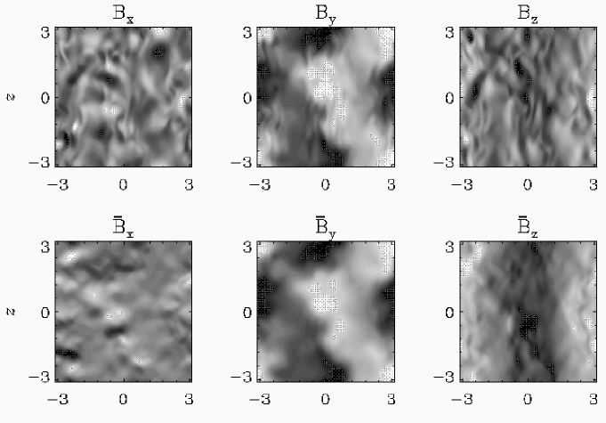
Longitudinal cross-sections show that the small scale contributions to the poloidal field result from variations in the toroidal direction. Whilst the toroidal field is relatively coherent in the toroidal direction, the poloidal field components are much less coherent and show significant fluctuations in the $y$-direction. We thus define mean fields $\overline{\mbox{\boldmath$B$}}$ to be the y-averaged fields. As can be seen from Figure 2 this is compatible with the definition of the mean field as the large-scale Fourier expansion. Two-dimensional power-spectra of this averaged field show that poloidal mean field components also gain significant power at the largest scale (i.e. at $\mbox{\boldmath$k$}{}^{2}<2$) at later times.

Figure 2.  : Images of the three components of $B$ in an arbitrarily chosen $xz$ plane (first row), compared with the $y$-averaged fields (second row). $120^{3}$ mesh-points, $t=5000$.

4 Helicity constraint and the mean magnetic field

In an unbounded or periodic system the magnetic helicity, $\langle\mbox{\boldmath$A$}{}\cdot\mbox{\boldmath$B$}{}\rangle$, evolves according to

$${{\rm d}{}\over{\rm d}{}t}\langle\mbox{\boldmath$A$}{}\cdot\mbox{\boldmath$B$}{}\rangle=-2\eta\langle\mbox{\boldmath$J$}{}\cdot\mbox{\boldmath$B$}{}\rangle.$$ (7)

Taking into account the spectral properties of the above quantities, we may separate large-scale and small-scale contributions and write

$$\langle\overline{\mbox{\boldmath$J$}}\cdot\overline{\mbox{\boldmath$B$}}\rangle/k_{1}\approx\mp B_{\rm tor}\,B_{\rm pol}\approx k_{1}\langle\overline{\mbox{\boldmath$A$}}\cdot\overline{\mbox{\boldmath$B$}}\rangle.$$ (8)

The expression above would for instance be true for a field of the form

$$\overline{\mbox{\boldmath$B$}}=\pmatrix{B_{\rm pol}\,\cos(k_{1}z+\varphi_{x})\cr B_{\rm tor}\,\sin(k_{1}z+\varphi_{y})\cr 0},$$ (9)

where we have allowed for an additional phase shift between the two components (relative to the already existing $\pi/2$ phase shift), $\varphi_{y}-\varphi_{x}$, but such a phase shift turned out to be small in our case. Furthermore, an additional $x$-dependence of the mean field, which is natural due to the $x$-dependence of the imposed shear profile could be accounted for. However, for the following argument all we need is relation (8). The amplitudes $B_{\rm pol}$ and $B_{\rm tor}$ can be calculated as

$$B_{\rm tor}\equiv\langle\overline{\mbox{\boldmath$B$}}_{y}^{2}\rangle^{1/2},\quad B_{\rm pol}\equiv\langle\overline{\mbox{\boldmath$B$}}_{x}^{2}+\overline{\mbox{\boldmath$B$}}_{z}^{2}\rangle^{1/2}.$$ (10)

Brackets denote here volume averaging while an overbar indicates an average over the toroidal direction ($y$). The upper sign applies to the present case where the kinetic helicity is positive (representative of the southern hemisphere), and the approximation becomes exact if Eq. (9) is valid.

Following B2000, in the steady case $\langle\mbox{\boldmath$A$}{}\cdot\mbox{\boldmath$B$}{}\rangle=\mbox{const}$, see Eq. (7), and so the r.h.s. of Eq. (7) must vanish, i.e. $\langle\mbox{\boldmath$J$}{}\cdot\mbox{\boldmath$B$}{}\rangle=0$, which can only be consistent with Eq. (8) if there is a small scale component, $\langle\mbox{\boldmath$j$}{}\cdot\mbox{\boldmath$b$}{}\rangle$, whose sign is opposite to that of $\langle\overline{\mbox{\boldmath$J$}}\cdot\overline{\mbox{\boldmath$B$}}\rangle$. Hence we write

$$\langle\mbox{\boldmath$J$}{}\cdot\mbox{\boldmath$B$}{}\rangle=\langle\overline{\mbox{\boldmath$J$}}\cdot\overline{\mbox{\boldmath$B$}}\rangle+\langle\mbox{\boldmath$j$}{}\cdot\mbox{\boldmath$b$}{}\rangle\approx 0.$$ (11)

This yields, analogously to B2000,

$$-{{\rm d}{}\over{\rm d}{}t}\left(B_{\rm tor}\,B_{\rm pol}\right)=+2\eta k_{1}^{2}\left(B_{\rm tor}\,B_{\rm pol}\right)-2\eta k_{1}|\langle\mbox{\boldmath$j$}{}\cdot\mbox{\boldmath$b$}{}\rangle|,$$ (12)

which yields the solution

$$B_{\rm tor}\,B_{\rm pol}=\epsilon_{0}B_{\rm eq}^{2}\left[1-e^{-2\eta k_{1}^{2}(t-t_{\rm s})}\right],$$ (13)

where $\epsilon_{0}=|\langle\mbox{\boldmath$j$}{}\cdot\mbox{\boldmath$b$}{}\rangle|/(k_{1}B_{\rm eq}^{2})$ is a prefactor, $B_{\rm eq}$ is the equipartition field strength with $B_{\rm eq}^{2}=\mu_{0}\langle\rho\mbox{\boldmath$u$}{}^{2}\rangle$, and $t_{\rm s}$ is the time when the small scale field has saturated which is when Eq. (12) becomes applicable. All this is equivalent to B2000, except that $\langle\overline{\mbox{\boldmath$B$}}^{2}\rangle$ is now replaced by the product $B_{\rm tor}\,B_{\rm pol}$. The significance of this expression is that large toroidal fields are now possible if the poloidal field is weak.

Figure 3.  : Growth of the product of poloidal and toroidal magnetic fields on a linear scale. The inset shows separately the evolution of poloidal and toroidal fields on a logarithmic scale. For the fit we have used $k_{1}^{2}=2$ and $\epsilon_{0}=3.8$.

In Figure 3 we show the evolution of the product $B_{\rm tor}\,B_{\rm pol}$ as defined in (10) and compare with Eq. (13). There are different stages; for $1200<t<2200$ and $3000<t<3700$ the effective value of $k_{1}^{2}$ is $2$ (because there are contributions from $k_{x}=1$ and $k_{z}=1$; see Figure 1), whilst at other times ($2500<t<2800$ and $t>4000$) the contribution from $k_{x}=1$ (for $2500<t<2800$) or $k_{z}=1$ (for $t>4000$) has become subdominant and we have effectively $k_{1}^{2}=1$. This is consistent with the change of field structure discussed in the previous section: for $2000<t<3000$ and around $t=4000$ the $B_{y}(k_{x}=1)$ mode is less powerful than the $B_{y}(k_{z}=1)$ mode.

5 Conclusions

The effects of the helicity constraint can clearly be identified in in our system even though much of the field amplification results from the shearing of a poloidal field. The constraint on the geometrical mean of the energies in the poloidal and toroidal field components is evident from Figure 3. The fit shows that the prefactor $\epsilon_{0}$ is about 3.8. Theoretically one may estimate $\epsilon_{0}$, which is proportional to $|\langle\mbox{\boldmath$j$}{}\cdot\mbox{\boldmath$b$}{}\rangle|$, by estimating $|\langle\mbox{\boldmath$j$}{}\cdot\mbox{\boldmath$b$}{}\rangle|\approx\rho_{0}|\langle\mbox{\boldmath$\omega$}{}\cdot\mbox{\boldmath$u$}{}\rangle|\approx k_{\rm f}\rho_{0}\langle\mbox{\boldmath$u$}{}^{2}\rangle\approx k_{\rm f}B_{\rm eq}^{2}$. Since $\epsilon_{0}=|\langle\mbox{\boldmath$j$}{}\cdot\mbox{\boldmath$b$}{}\rangle|/(k_{1}B_{\rm eq}^{2})$ this yields $\epsilon_{0}\approx k_{\rm f}|/k_{1}=5$, in good agreement with the simulation.

Power spectra of the poloidal field show that most of the power is in the small scales, making the use of averages at first glance questionable. However, once the field is averaged over the toroidal direction the resulting poloidal field is governed by large scale patterns (the slope of the spectrum is steeper than $k^{-1}$, which is the critical slope for equipartition). The presence even of a weak poloidal field is crucial for understanding the resulting large scale field generation in the framework of an $\alpha\Omega$ dynamo.

In another paper (Brandenburg et al. 2000) we have elaborated further on the similarity between the present simulations and $\alpha\Omega$ dynamos. In particular, we have discussed anisotropic turbulent magnetic diffusivities as a possible explanation for the difference between the resistive growth time of the field on the one hand and a shorter cycle period seen in the simulation on the other. With just one simulations so far it is impossible to verify any scaling, but it is worth mentioning that the present cycle time of around 1000 time units is close to the geometrical mean of resistive and dynamical timescales. Nevertheless, one must not forget that the real sun does have open boundaries, and it is now important to understand their role on the magnetic helicity constraint.

References

- [] Berger, M. A., & Ruzmaikin, A. (2000) Rate of helicity production by solar rotation. J. Geophys. Res. 105, 10481–10490
- [] Blackman, E. G., & Field, G. F. (2000) Constraints on the Magnitude of alpha in Dynamo Theory. Astrophys. J. 534, 984–988
- [] Brandenburg, A. (2000)“The inverse cascade and nonlinear alpha-effect in simulations of isotropic helical hydromagnetic turbulence,” Astrophys. J. (in press) (astro-ph/0006186)
- [] Brandenburg, A. & Subramanian, K. (2000) Large scale dynamos with ambipolar diffusion nonlinearity. Astron. Astrophys. 361, L33–L36
- [] Brandenburg, A., Bigazzi, A., & Subramanian, K. (2000) The helicity constraint in turbulent dynamos with shear, Mon. Not. Roy. Astron. Soc. (submitted), (astro-ph/0011081)
- [] Brandenburg, A., Nordlund, Å., Stein, R. F., & Torkelsson, U. (1995) Dynamo-generated Turbulence and Large-Scale Magnetic Fields in a Keplerian Shear Flow. Astrophys. J. 446, 741–754
- [] Glatzmaier, G. A., & Roberts, P. H. (1995) A three-dimensional self-consistent computer simulation of a geomagnetic field reversal. Nature 377, 203–209
- [] Kleeorin, N. I, Moss, D., Rogachevskii, I., & Sokoloff, D. (2000) Helicity balance and steady-state strength of the dynamo generated galactic magnetic field. Astron. Astrophys. 361, L5–L8
- [] Krause, F., & Rädler, K.-H. (1980) Mean-Field Magnetohydrodynamics and Dynamo Theory. Pergamon Press, Oxford
- [] Moffatt, H. K. (1978) Magnetic Field Generation in Electrically Conducting Fluids. CUP, Cambridge