Cluster abundance and large scale structure

Abstract

We use the presently observed number density of large X-ray clusters and the linear mass power spectra from galaxy surveys to constrain the amplitude of matter density perturbations on the scale of $8h^{-1}$Mpc ($\sigma_{8}$), and the redshift distortion parameter ($\beta$), in both open cosmologies and flat models with a non-zero cosmological constant. The best fit to the observed mass power spectra gives $n=0.84\pm 0.67$ and $\Gamma=0.27^{+0.42}_{-0.16}$, with the theoretically expected degeneracy $\Gamma^{\prime}=0.247\Gamma\exp(1.4n)=0.220^{+0.036}_{-0.031}$ (all at 95 per cent confidence level). These are consistent with the recent CMB results. Based on this, we then calculate the cluster-abundance-normalized $\sigma_{8}$, using different models of mass function. The models considered are by Press & Schechter (PS; 1974), by Sheth & Tormen (ST; 1999), and by Lee & Shandarin (LS; 1999). The last two incorporate non-spherical gravitational collapse, and the $\sigma_{8}$ based on these two models are significantly lower. This lower normalization results from the larger mass function within the scale range of our interest. In particular, we combine the results of these two models to yield $\sigma_{8{\rm(ST+LS)}}=0.477\Omega_{\rm m0}^{\alpha}$, where $\alpha=-0.3-0.17\Omega_{\rm m0}^{0.34}-0.13\Omega_{\Lambda 0}$. In our analysis, we also derive the probability distribution function of cluster formation redshift using the Lacey-Cole formalism (1993), but with modifications to incorporate non-spherical collapse. The origins of uncertainties in our $\sigma_{8}$ results are also investigated separately, with the main contributer being the normalization in the virial mass-temperature relation. From the PSCz power spectrum alone and using $\Gamma^{\prime}=0.220^{+0.036}_{-0.031}$ as the prior, we also obtain for the IRAS galaxies $\sigma_{8\rm(I)}=0.78\pm 0.06$ (at 95 per cent confidence level) . By combining this with the $\sigma_{8}$ result, we are able to constrain the redshift distortion parameter $\beta_{\rm I}$, which is in turn lower in the non-spherical-collapse models. We found $\beta_{\rm I(ST+LS)}=0.613\Omega_{\rm m0}^{0.24-0.16(\Omega_{\rm m0}+\Omega_{\Lambda 0})}$. This is more consistent with the recent observations than the result based on the PS formalism.

1 Introduction

One of the most important constraints on models of structure formation is the observed abundance of galaxy clusters. Because they are the largest virialized objects in the universe, their abundance can be simply predicted by linear perturbation theory. In the literature, the cluster abundance has been widely used to constrain different cosmological models [White, Efstathiou & Frenk 1993a, Eke, Cole & Frenk 1996, Viana & Liddle 1999, Kitayama & Suto 1997, Wang & Steinhardt 1998, Avelino, Wu & Shellard 2000]. Here, we shall consider its constraint on the amplitude of matter density perturbations on the scale of $8h^{-1}$Mpc, $\sigma_{8}$, and the redshift distortion parameter, $\beta$, in the standard inflationary models. This requires the knowledge about the linear power spectrum of mass perturbations, the so-called ‘mass function’ (the differential number density of collapsed objects as a function of mass), the probability distribution function of cluster formation redshift, and the virial mass-temperature relation. Although this has been studied by many other authors [Viana & Liddle 1999, Eke, Cole & Frenk 1996, Wang & Steinhardt 1998, Borgani et al. 1999, Pierpaoli, Scott & White 2000], we revisit this problem with more caution to incorporate the recent progress in measuring the linear mass power spectrum, as well as understanding the mass function. Based on these new developments, we shall investigate $\sigma_{8}$ and $\beta$ in both open cosmologies and flat models with a non-zero cosmological constant.

The structure of the paper is as follows. In section 2, we first investigate the observed linear mass power spectra. This includes the estimation of $\sigma_{8}$, the spectral index $n$, and the shape parameter $\Gamma$. They parameterize the linear mass power spectrum predicted by the standard inflationary models. Within such models, we reveal the degeneracy between $n$ and $\Gamma$, and thus reparameterize the linear mass power spectrum with only a single parameter, the degenerated shape parameter $\Gamma^{\prime}$. The IRAS $\sigma_{8{\rm(I)}}$ is also estimated here. In section 3, we explore different models of mass function. The models considered are by Press & Schechter (PS; 1974), by Sheth & Tormen (ST; 1999), and by Lee & Shandarin (LS; 1999), the last two of which incorporate non-spherical collapse. In section 4, we then derive the probability distribution function of cluster formation redshift for different models of mass function. The formalism employed is by Lacey & Cole (1993, 1994), but modified to incorporate non-spherical collapse. In section 5, we describe how the virial mass of different formation redshift is related to its temperature, and lay down the formalism that relates $\sigma_{8}$ to the cluster abundance. In section 6, we first calculate the $\sigma_{8}$ normalized to the observed cluster abundance. We present the estimates of the $\sigma_{8}$ based on different models of mass function, and compare these results with other work in the literature. The uncertainties of our results are investigated, with an explicit form for the dependence on various error sources. We further show how to derive $\beta$ from the information we have, and compare our results with recent observations. Finally, in section 7, we give a brief conclusion.

2 Matter perturbations and power spectrum

The standard deviation of matter density perturbations at a smoothing scale $R$ is related to the mass power spectrum ${\cal P}(k)$ as

$$\sigma^{2}(R)=\int|w(kR)|^{2}S(k)\frac{dk}{k},$$ (1)

where $w(x)$ is the Fourier transform of an unit top-hat spherical window:

$$w(x)=\frac{3(\sin x-x\cos x)}{x^{3}},$$ (2)

and

$$S(k)=\frac{k^{3}}{2\pi^{2}}{\cal P}(k),$$ (3)

which is dimensionless and thus independent of the units of $k$. We shall use $h^{-1}$Mpc and $h$Mpc^-1 as the units of $R$ and $k$ respectively, where $h$ is the present Hubble parameter $H_{0}$ in units of $100$ km s^-1Mpc^-1. A subscript ‘0’ will denote a quantity evaluated at the present epoch. Theoretically, the matter power spectrum ${\cal P}(k)$ in adiabatic inflationary models can be expressed as

$${\cal P}(k)\propto k^{n}T^{2}(k),$$ (4)

where $n$ is the ‘spectral index’, which specifies the scale dependence of the initial perturbations, and $T(k)$ is the ‘transfer function’, which transfers the initial perturbations to the present epoch. An accurate and analytically motivated form of $T(k)$ is [Eisenstein & Hu 1998]

$$T(k)=\left\{1+\frac{\left[14.2+731/(1+62.5q)\right]q^{2}}{\textrm{ln}(2e+1.8q)}\right\}^{-1},$$ (5)

where $q=k/\Gamma$ ($q$ is originally defined in units normalized to the inverse of the horizon size at the epoch of radiation-matter-energy-density equality), and [Sugiyama 1995]

$$\Gamma=\Omega_{\rm m0}h\exp(-\Omega_{\rm B0}-\frac{\Omega_{\rm B0}}{\Omega_{\rm m0}})\,.$$ (6)

Here $\Omega_{\rm m0}$ and $\Omega_{\rm B0}$ are the present matter and baryon energy densities respectively. For a fixed $n$, $\Gamma$ determines the location of the broad peak in ${\cal P}(k)$, and thus the name ‘shape parameter’. In the analysis of later sections, we shall use $\Omega_{\rm B0}=0.05$, and then investigate the dependence of our final results on this.

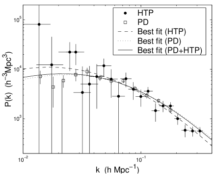
From the theoretical modeling (4), we see that the shape of ${\cal P}(k)$ has two essential parameters, $n$ and $\Gamma$, i.e., ${\cal P}(k)\equiv{\cal P}(k;n,\Gamma)$. Thus a comparison between this modeling and observations will give us some estimates of $n$ and $\Gamma$. The observations we considered are the linear mass power spectrum ${\cal P}_{\rm(PD)}(k)$ by Peacock and Dodds (1994; hereafter PD), which was compiled from surveys of different classes of galaxies and galaxy clusters, and the decorrelated linear IRAS galaxy-galaxy power spectrum ${\cal P}_{\rm I(HTP)}(k)$ by Hamilton, Tegmark, and Padmanabhan (2000; hereafter HTP), which was based on the IRAS Point Source Catalogue Redshift Survey (PSCz; Saunders et al. 2000). As advised by the authors, to avoid the effect of non-linear evolution on smaller scales (larger $k$), we used only the first twelve data points of PD ($k\mathrel{\hbox to0.0pt{\lower 4.0pt\hbox{\hskip 1.0pt$\sim$}\hss}\raise 1.0pt\hbox{$<$}}0.2h$Mpc^-1), and the first twenty two data points of HTP ($k\mathrel{\hbox to0.0pt{\lower 4.0pt\hbox{\hskip 1.0pt$\sim$}\hss}\raise 1.0pt\hbox{$<$}}0.3h$Mpc^-1). They are shown in figure 1 as squares and dots respectively (with associated error bars). Using the maximum-likelihood method based on a $\chi^{2}$ analysis, the results of the best estimates are shown in table 1 and figure 1.

In table 1, all the errors are at 95 per cent confidence level. The last column gives the $\chi^{2}$ values of the best fits, the degrees of freedom (DOF) in the analysis, and their corresponding confidence levels (CL). In obtaining the results for the HTP (the bracketed numbers), we have used a top-hat prior $2\geq n\geq 0$ (see later for reasons). In figure 1, the best fits of ${\cal P}(k)$ for PD and HTP are shown as the dotted and dashed lines respectively. When compared with the HTP (dots and dashed line), the more constraining feature in the PD data (squares) on larger scales (smaller $k$) tends to confine the peak of the best-estimated ${\cal P}(k)$ (dotted line) to smaller scales (larger $k$), and thus a larger estimate of $\Gamma$ (see table 1).

Figure 1: Mass power spectra of different observations and their best fits (see text for details).

	$n$	$\Gamma$	$\Gamma^{\prime}$	$\chi^{2}$/DOF (CL)
HTP	$\!\!\!\left(0.91^{+1.09}_{-0.91}\right)$	$\!\!\!\left(0.18^{+0.74}_{-0.18}\right)$	$\!\!\!0.160^{+0.085}_{-0.051}$	15.4/19 (70%)
PD	$\!\!\!0.99^{+0.81}_{-0.86}$	$\!\!\!0.23^{+0.55}_{-0.16}$	$\!\!\!0.229^{+0.042}_{-0.033}$	6.95/9 (64%)
HTP+PD	$\!\!\!0.84^{+0.67}_{-0.67}$	$\!\!\!0.27^{+0.42}_{-0.16}$	$\!\!\!0.220^{+0.036}_{-0.031}$	24.6/30 (74%)

Table 1: Best fits of different LSS data sets. The errors are at 95 per cent confidence level. The bracketed numbers were obtained using a prior $2\geq n\geq 0$. See text for more details.

We then combined both the HTP and PD into the same likelihood analysis (denoted as HTP+PD) with all data points equally weighted. In the combined analysis, we allowed a galaxy-to-mass bias in the HTP spectrum to vary:

$$b_{\rm I(HTP)}=\left[\frac{{\cal P}_{\rm I(HTP)}(k)}{{\cal P}_{\rm(HTP)}(k)}\right]^{1/2},$$ (7)

while fixing the amplitude of ${\cal P}_{\rm(PD)}(k)$. The best fit of HTP+PD showed (at 95 per cent confidence level)

$$b_{\rm I(HTP)}=1.28^{+0.21}_{-0.18}.$$ (8)

This value also implies the bias between the HTP IRAS galaxy power spectrum and the PD mass power spectrum. We note in figure 1 that for a direct comparison, we have rescaled down the amplitudes of the HTP data (dots with crosses) and their best fit (the dashed line) by a factor of $b_{\rm I(HTP)}^{2}=1.28^{2}$.

The estimates of $\Gamma$ and $n$ from the HTP+PS are shown in table 1. The corresponding best fit of ${\cal P}(k)$ is plotted as the solid line in figure 1. We see that it is much closer to the best fit of PD (the dotted line), and this is mainly due to the smaller error bars in the PD. From the last column of table 1, we also see that the best fits of each case (HTP, PS, and HTP+PS) are good, and agree well with each other. Based on the form (6) of $\Gamma$, it is worth emphasizing that our estimates of $\Gamma$ and $n$ are consistent with the recent CMB constraints, which give $0.3\mathrel{\hbox to0.0pt{\lower 4.0pt\hbox{\hskip 1.0pt$\sim$}\hss}\raise 1.0pt\hbox{$>$}}\Gamma\mathrel{\hbox to0.0pt{\lower 4.0pt\hbox{\hskip 1.0pt$\sim$}\hss}\raise 1.0pt\hbox{$>$}}0.1$ and $n\approx 1$ [Balbi et al. 2000, Lange et al. 2000, Jaffe et al. 2000].

Figure 2: The 68%, 95%, and 99% contours (inner out) of the maximum-likelihood analysis for the parameters $\Gamma$ and $n$, based on the PD (dashed), HTP (dotted), and HTP+PD (shaded). The strong degeneracy between $\Gamma$ and $n$ is apparent. The square, circle, and cross label the best fit of each case shown in table 1.

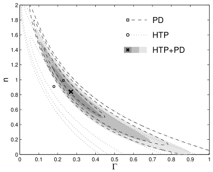
One interesting observation in all the above likelihood analyses is that there is a strong degeneracy between the estimates of $n$ and $\Gamma$: the larger the $\Gamma$, the smaller the $n$. Figure 2 shows this degeneracy in the likelihood plots of the three cases (PD, HTP, and HTP+PD). For any $n$ within $2\geq n\geq 0$, we found that the $\Gamma$ of local maximum likelihood can be well fitted by

$$\Gamma=\cases{0.657\exp(-1.38n-0.02n^{6})&for HTP,\cr 0.912\exp(-1.38n-0.002n^{6})&for PD,\cr 0.868\exp(-1.38n-0.002n^{6})&for HTP+PD,\cr}$$ (9)

all within 3% error. This degeneracy is caused by the fact that ${\cal P}(k)$ is lack of feature except a broad peak, so that in producing the same shape of ${\cal P}(k)$ a larger $\Gamma$ (which tends to shift the peak to the right) can compensate for a smaller $n$ (which tends to shift the peak to the left). This is theoretically expected as can be seen from equations (4) and (5). Thus such a degeneracy allows us to write

$${\cal P}(k;n,\Gamma)\propto{\cal P}(k;1,\Gamma^{\prime}),$$ (10)

with the ‘degenerated shape parameter’

$$\Gamma^{\prime}\equiv\Gamma^{\prime}(n,\Gamma)=\Gamma\exp(1.4n-1.4)\approx 0.247\Gamma\exp(1.4n),$$ (11)

which equals the shape parameter $\Gamma$ when $n=1$. We verified that this parameterization is accurate within 10% error (when ${\cal P}(k)$ is normalized at $k=0.2h$Mpc^-1) for $1.4>n>0.5$, $0.6>\Gamma>0.09$, $0.28>\Gamma^{\prime}>0.15$, and $0.01>k/(h$Mpc${}^{-1})>0.3$ (the range of linear scales probed by observations). Using this parameterization, we obtained the best fits of $\Gamma^{\prime}$ shown in table 1. We note that with the degeneracy (11) the best fits of $\Gamma^{\prime}$ are consistent with those of the $n$ and $\Gamma$. When comparing the best fits of $\Gamma^{\prime}$ in HTP, PD, and HTP+PD, we also note that the larger values of $\Gamma^{\prime}$ in the HTP+PD and PD analyses reflect the previously observed fact that the peak in ${\cal P}(k)$ is confined to smaller scales (larger $k$) in these two cases (see figure 1). In the rest of our analysis, we shall use the parameterization (10), and adopt the result of HTP+PD. Its errors can be well approximated by a log-normal distribution (at 95 per cent confidence level; c.f., table 1)

$$\Gamma^{\prime}=0.220^{+0.036}_{-0.031}\approx 0.220\times 10^{\pm 0.066}.$$ (12)

In principle, we can also use observations to constrain $\sigma_{8}$ via equation (1). However, this is forbidden by the large uncertainty in the normalization of mass power spectrum, mainly resulted from the large uncertainty in the understanding of the galaxy to mass bias. Hence, instead, we shall use the abundance of X-ray clusters to constrain $\sigma_{8}$, as is one of the main goals of this paper. Nevertheless, here we can still use ${\cal P}_{{\rm I(HTP)}}$ alone to constrain the $\sigma_{8}$ for the IRAS galaxies, namely $\sigma_{8{\rm(I)}}$. A maximum-likelihood method with equation (12) as a prior gives an estimate

$$\sigma_{8{\rm(I)}}=0.78\pm 0.03,$$ (13)

at 68 per cent confidence level, and $\sigma_{8{\rm(I)}}=0.78\pm 0.06$ at 95 per cent confidence level. This result will be used in Section 6.3 for the discussion of redshift distortion parameter.

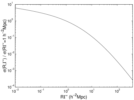
We now investigate the scale dependence of the amplitude of matter perturbations. By using equation (1) together with equations (4) and (5), we obtained a numerical fit

$$\sigma(R;n=1,\Gamma)=\sigma_{8}\frac{\varrho(R\Gamma)}{\varrho(8\Gamma)},$$ (14)

where $\sigma_{8}\equiv\sigma(R=8)$, and

$$\varrho(r)=r^{-\psi(r)},\,~{}~{}\psi(r)=0.3+\frac{1.45}{1+\left(20/r\right)^{0.35}}.$$ (15)

Alternatively, we have

$$R(\sigma;n=1,\Gamma)=\Gamma^{-1}{\zeta(\frac{\sigma}{\sigma_{8}}\varrho(8\Gamma))},$$ (16)

where

$$\zeta(s)\equiv\varrho^{-1}\approx 5.2s^{-0.53}\exp\left(\frac{-s^{0.63}}{0.6}\right).$$ (17)

Here $\varrho^{-1}$ means the inverse function of $\varrho$, which is defined in equation (15). These fits (eqs. [14] and [16]) are accurate within $5\%$ error for $1000>R\Gamma>0.01$. We also note that the coupling of $R$ and $\Gamma$ in these fits is theoretically required (see eqs. [1] and [5] with the fact that $q=k/\Gamma$). To account for the dependence of $\sigma(R)$ on $n$, we can simply replace the $\Gamma$ in equation (14) with $\Gamma^{\prime}$ (see also eq. [10] and context), i.e.,

$$\sigma(R;n,\Gamma)=\sigma(R;n=1,\Gamma^{\prime})=\sigma_{8}\frac{\varrho(R\Gamma^{\prime})}{\varrho(8\Gamma^{\prime})}.$$ (18)

The dependence of $\sigma$ on $R$ and $\Gamma^{\prime}$ is shown in figure 3.

Figure 3: Dependence of amplitude of mass perturbations $\sigma$ on the smoothing scale $R$ and the degenerated shape parameter $\Gamma^{\prime}$.

In the later discussion, we shall also need the red-shift dependence of $\sigma$ for a given present value in a given background cosmology. This can be described accurately by

$$\sigma(R,z)=\sigma(R,z=0)\frac{g(\Omega_{\rm m},\Omega_{\Lambda})}{(1+z)g(\Omega_{\rm m0},\Omega_{\Lambda 0})},$$ (19)

where $z$ is the red-shift, $\Omega_{\Lambda}$ is the energy density of the cosmological constant $\Lambda$, and [Carroll, Press & Turner 1992]

$$g(\Omega_{\rm m},\Omega_{\Lambda})=\frac{2.5\Omega_{\rm m}}{\left[\Omega_{\rm m}^{4/7}-\Omega_{\Lambda}+(1+{\Omega_{\rm m}/2})(1+{\Omega_{\Lambda}/70})\right]},$$ (20)

which accounts for the discrepancy of the growing behavior of matter perturbations from that of a critical-density universe. An analytical expression for the evolution of $\Omega_{\rm m}$ is

$$\Omega_{\rm m}\equiv\Omega_{\rm m}(z)=\frac{\Omega_{\rm m0}(1+z)^{3}}{(1+z)^{2}(1+\Omega_{\rm m0}z-\Omega_{\Lambda 0})+\Omega_{\Lambda 0}}.$$ (21)

Throughout this paper, we shall investigate open models with $\Omega_{\rm m}<1$ and $\Omega_{\Lambda}=0$ (denoted as OCDM hereafter), and flat models with $\Omega_{\rm m}+\Omega_{\Lambda}=\Omega_{\rm m0}+\Omega_{\Lambda 0}=1$ (denoted as $\Lambda$CDM hereafter).

3 The mass function

To apply constraint from the observed cluster abundance onto the amplitude of matter perturbations $\sigma(R)$, we first need to relate it to the number density of clusters. By definition, the fraction of the total mass within collapsed objects larger than a given mass $M$ at a red-shift $z$ is

$${\cal F}(M(R,z),z)={{\Omega_{\rm m}(>M(R,z),z)}\over{\Omega_{\rm m}(z)}}.$$ (22)

Here $M(R,z)$ is the cluster mass of a corresponding scale $R$ and is defined by

$$M(R,z)=\frac{4}{3}\pi R^{3}\overline{\rho}(z),$$ (23)

where $\overline{\rho}(z)$ is the average energy density of the universe at red-shift $z$. With the numbers given in [Kolb & Turner 1990], we obtain

$$M(R,0)=1.162\times 10^{12}R^{3}\Omega_{\rm m0}h^{-1}{\rm M}_{\odot},$$ (24)

where $R$ is in $h^{-1}$Mpc and ${\rm M}_{\odot}$ is the solar mass. Thus the differential number density of clusters at a mass interval $dM$ about $M$ can be derived as:

$$n_{i}(M,z)dM=-F_{i}(\mu)\frac{\overline{\rho}}{M\sigma}\frac{d\sigma}{dM}dM,\quad i=\textrm{PS, ST, or LS},$$ (25)

where $\sigma\equiv\sigma(R,z)$, $\overline{\rho}\equiv\overline{\rho}(z)$, $\mu\equiv\mu(\sigma)$, and

$$F_{i}(\mu)=\frac{d{\cal F}(M(R,z),z)}{d{\rm ln}\sigma(R,z)}.$$ (26)

The $n_{i}$ in equation (25) is normally referred as the ‘mass function’. In different models of mass function, the $F_{i}(\mu)$ (and therefore $n_{i}$) has different forms. Here we shall consider the models by Press & Schechter (1974; hereafter PS), by Sheth & Tormen (1999; hereafter ST), and by Lee & Shandarin (1999; hereafter LS):

$$F_{\rm PS}(\mu)=\sqrt{\frac{2}{\pi}}\mu\exp\Big{(}-\frac{\mu^{2}}{2}\Big{)},$$ (27)

with $\mu=\delta_{\rm c}/{\sigma}$ and $\delta_{\rm c}=1.68647$;

$$F_{\rm ST}(\mu)=0.322\sqrt{\frac{2}{\pi}}\left(1+\frac{1}{\nu^{0.6}}\right)\nu\exp\Big{(}-\frac{\nu^{2}}{2}\Big{)},$$ (28)

with $\nu=\sqrt{0.707}\mu$, $\mu=\delta_{\rm c}/{\sigma}$, and $\delta_{\rm c}=1.68647$; and

$$F_{\rm LS}(\mu)=\frac{25\sqrt{10}}{2\sqrt{\pi}}\mu\Bigg{[}\Big{(}\frac{5\mu^{2}}{3}-\frac{1}{12}\Big{)}\exp\Big{(}-\frac{5\mu^{2}}{2}\Big{)}\times$$

$${\rm erfc}\Big{(}{\sqrt{2}\mu}\Big{)}+\frac{\sqrt{6}}{8}\exp\Big{(}-\frac{15\mu^{2}}{4}\Big{)}\times$$

$${\rm erfc}\Big{(}\frac{\sqrt{3}\mu}{2}\Big{)}-\frac{5\sqrt{2\pi}\mu}{6\pi}\exp\Big{(}-\frac{9\mu^{2}}{2}\Big{)}\Bigg{]},$$ (29)

with $\mu=\lambda_{\rm 3c}/{\sigma}$ and $\lambda_{\rm 3c}=0.37$.

The $n_{\rm\scriptscriptstyle PS}$ is based on the Press-Schechter formalism, which relates the mass fraction of collapsed objects whose mass is larger than some given threshold $M$, with the fraction of space in which the evolved linear density field exceeds some threshold $\delta_{\rm c}$. It has been extensively tested against N-body simulations with considerable success, but recently found to have steeper shape tilted towards larger mass $M$. This is mainly due to the spherical-collapse assumption in the PS formalism (while simulations showed that non-spherical collapses are important in the clustering process), and the fact that peaks in a linear field are poorly correlated with the final spatial locations of dark halos (for a review, see Lee & Shandarin 1999 and references therein). The $n_{\rm\scriptscriptstyle ST}$ by Sheth & Tormen (1999) was first obtained as a numerical fit to simulations. Sheth, Mo & Tormen (1999) then showed that it could be associated with a model of ellipsoidal, rather than spherical collapse. The $n_{\rm\scriptscriptstyle LS}$ by Lee & Shandarin (1999) is a full analytical alternative of $n_{\rm\scriptscriptstyle PS}$. It incorporates non-spherical dynamics and assumes that dark halos form in the local maxima of the smallest eigenvalue of the deformation tensor $\lambda_{\rm 3c}$. It has been shown to be in better agreement with simulations than the PS formalism [Lee & Shandarin 1999].

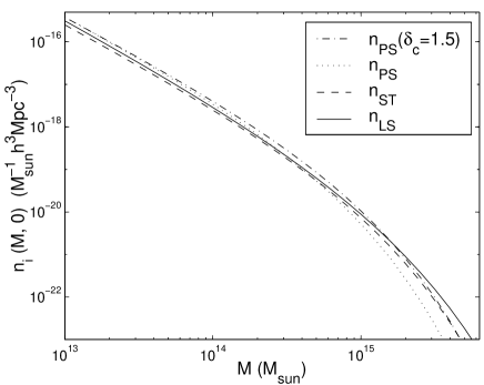
Figure 4 shows the mass functions $n_{i}$ of these three models. It indicates that the PS mass function (dotted line) predicts fewer massive clusters and more light clusters than the ST and LS mass functions (dashed and solid lines respectively). In the literature, it has been shown that the PS formalism with a smaller $\delta_{c}$ can produce more massive clusters and thus resemble the simulations better for large $M$, but still suffers from the overestimate of light objects [Tormen 1998, Lee & Shandarin 1999]. To show this effect, in figure 4 we plotted another PS mass function with $\delta_{c}=1.5$ (dot-dashed line) for comparison. In addition, we should also note that the $\delta_{c}$ is fixed by the fit to the global mass function, and therefore not a free parameter essentially.

Figure 4: The mass function $n_{i}$ (the differential number density of collapsed objects within a mass interval $dM$ about $M$) of different models ($i=$PS, ST, and LS). See equation (25) and context for details.

Finally, substituting equation (18) together with (15) into (25) (see also eq. [19]), we obtain the present cluster abundance as

$$n_{i}(M,0)=F_{i}(\mu)\frac{\overline{\rho}}{3M^{2}}\left\{\gamma(R\Gamma)+\frac{1.45(R\Gamma)^{0.35}\log(R\Gamma)}{[(R\Gamma)^{0.35}+2.85]^{2}}\right\}.$$ (30)

We note that the $\sigma_{8}$ dependence of $n_{i}(M,0)$ here has now been implicitly embedded into the $\mu(\sigma)$ of $F_{i}(\mu)$, as well as the $M$ and $R$ through equations (16) and (23).

4 Formation redshift of clusters

While the cluster abundance in our theoretical formalism (eq. [30]) is a function of the cluster mass, the observed abundance of X-ray clusters is normally in the form of a function of the X-ray temperature. Therefore, we need to relate the X-ray temperature $T$ of a cluster with its virial mass $M_{\rm v}$. Since clusters of the same mass may have formed at different red-shifts resulting in different present temperatures, we first need to decompose the present number density of clusters of given mass into contributions from different formation time, and then relate the virial mass of a formation time with the present temperature. That is, we first need to find out how much of the present abundance $n_{i}(M,z=0)$ of given mass $M$ was formed at a given redshift $z$, and then associate this abundance with the temperature that corresponds to the given $M$ and $z$. In this section, we shall discuss the first step, while leaving the second step to the next section.

To achieve the first step, we need to know the probability that a cluster of given present mass was formed at the given redshift. Lacey and Cole constructed a merging history for dark matter halos based on the excursion set approach and obtained an analytical expression for the probability that a galaxy cluster with present virial mass $M$ would have formed at the given red-shift $z$ (Lacey & Cole 1993, 1994). Here we shall generalize their formalism in the following way to incorporate different models of mass function. At first, the probability that the formation time of a halo of mass $M_{0}$ at $z_{0}$ was earlier than $z$ equals the probability that it had a parent of mass $M>fM_{0}$ at redshift $z$, where $f$ is the fraction of the cluster mass assembled by redshift $z$. This probability can be easily obtained by a halo counting argument (modified from Lacey & Cole 1993):

$$P(M>fM_{0},z|M_{0},z_{0})=\int_{S_{0}}^{S_{f}}\frac{M_{0}}{M(S)}\frac{F_{i}(\mu)}{2(S-S_{0})}dS,$$ (31)

where $S\equiv S(M)=\sigma^{2}(M,z=0)$, $S_{0}\equiv S(M_{0})$, $S_{f}\equiv S(fM_{0})$, and $\mu=\delta_{\rm c}[\sigma(M,0)/\sigma(M,z)-1]/\sqrt{S-S_{0}}$ (the $\delta_{\rm c}$ here should be replaced with $\lambda_{\rm 3c}$ for the LS formalism, and the same applies to the later appearance of $\delta_{\rm c}$ in this section). Therefore the probability that a galaxy cluster with present virial mass $M$ was formed at a given $z$ can be obtained as:

$$p_{z}(z)=-\frac{\partial P(M>fM_{0},z|M_{0},z_{0})}{\partial z}.$$ (32)

With the change of variables

$$s=\frac{S-S_{0}}{S_{f}-S_{0}},\quad{\omega}=\frac{\delta_{\rm c}[\sigma(M,0)/\sigma(M,z)-1]}{\sqrt{S_{f}-S_{0}}},$$ (33)

equation (32) can be rewritten as

$$p_{z}(z)=p_{\omega}(\omega)\frac{\partial\omega}{\partial z},$$ (34)

where

$$p_{\omega}(\omega)=-\frac{\partial P}{\partial\omega}=-\int_{0}^{1}\left[\frac{R_{0}}{R(\sigma)}\right]^{3}\frac{\partial F_{i}(\mu)}{\partial\mu}\frac{ds}{2s^{3/2}},$$ (35)

and

$$\mu=\frac{\omega}{\sqrt{s}},\quad\sigma\equiv\sigma(M,z=0)=\left[s(S_{f}-S_{0})+S_{0}\right]^{1/2}.$$ (36)

Here $R_{0}$ can be obtained from equation (24) by taking $M=M_{0}$, and $R(\sigma)$ is given either by equation (16) for inflationary CDM models, or by $R\propto\sigma^{-2/(n_{\rm s}+3)}$ for power-law-spectrum models with $P(k)\propto k^{n_{\rm s}}$. In the latter case, we have $\left[R_{0}/R(\sigma)\right]^{3}=\left[1+s(f^{-(n_{\rm s}+3)/3}-1)\right]^{3/(n_{\rm s}+3)}$. Under certain conditions, equation (35) can be analytically integrated to yield an explicit expression of $p_{\omega}(\omega)$. For example, for power-law-spectrum models with $n_{\rm s}=0$, we have simply $\left[R_{0}/R(\sigma)\right]^{3}=1+s(f^{-1}-1)$. Thus we obtain for PS

$$\begin{array}[]{ll}p_{\omega}(\omega)=&2\omega(f^{-1}-1){\rm erfc}\left({\omega\over\sqrt{2}}\right)-\\ &{\sqrt{2\over\pi}}(f^{-1}-2)\exp\left(-{{\omega^{2}}\over 2}\right),\end{array}$$ (39)

and the result for ST can be also straightforwardly obtained.

The form of equation (35) is general and thus suitable for any given model of mass function. Once given the mass function, which is specified by $F_{i}(\mu)$ (see eq. [25]), we can first use equation (35) to obtain $p_{\omega}$, and then equation (34) to get $p_{z}(z)$. From equations (33), (34), and (19), we first note that for $\Omega_{\rm m0}=1$ and $\Lambda=0$, $\omega(z)$ is proportional to $z$, so that the conversion from $p_{\omega}(\omega)$ to $p_{z}(z)$ requires only a linear rescale in both $\omega$ and $p_{\omega}(\omega)$. Even for other values of $\Omega_{\rm m0}$ and $\Lambda$, which result in non-linear conversion from $\omega$ to $z$ and thus from $p_{\omega}(\omega)$ to $p_{z}(z)$, the relative ratios between the $p_{z}(z)$ of the PS, ST and LS formalisms will remain the same as in the $p_{\omega}(\omega)$, i.e. the conversion from $p_{\omega}(\omega)$ to $p_{z}(z)$ is independent of the choice of the mass function. This allows us to directly compare the $p_{\omega}(\omega)$ of PS, ST and LS, and keep the conclusions still available for $p_{z}(z)$. Figure 5 shows the $p_{\omega}(\omega)$ in the PS (dotted lines), ST (dashed lines), and LS (solid lines) formalisms, for power-law-spectrum models with $n_{\rm s}=-2,-1,0$ and $1$. For a direct comparison, we have rescaled the $p_{\omega}(\omega)$ of ST with $\lambda_{\rm 3c}/\delta_{\rm c}$, and its $\omega$ with $\delta_{\rm c}/\lambda_{\rm 3c}$, due to the fact that $\omega\propto\delta_{\rm c}$, $\lambda_{\rm 3c}$ (see eq. [33]). We have also verified that for the inflationary CDM models, the $p_{\omega}(\omega)$ (and thus $p_{z}(z)$) of a chosen mass function approximately interpolates between those based on the pow-law-spectrum models. We should also notice that the PS results here (the dotted lines) are identical to those presented in Lacey & Cole (1993).

Figure 5: The probability distribution $p_{\omega}(\omega)$ of halo formation epochs $\omega(z)$ calculated from equation (35) of different models, for power-law spectra with $n_{\rm s}=-2$, $-1$, $0$ and 1 (from bottom to top at $\omega=1$). For a direct comparison, we have rescaled the $p_{\omega}(\omega)$ of ST with $\lambda_{\rm 3c}/\delta_{\rm c}$, and its $\omega$ with $\delta_{\rm c}/\lambda_{\rm 3c}$, due to the fact that $\omega\propto\delta_{\rm c}$, $\lambda_{\rm 3c}$. Here we have used $f=0.5$. We also note that $\omega(z)\propto z$ when $\Omega_{\rm m0}=1$ and $\Lambda=0$.

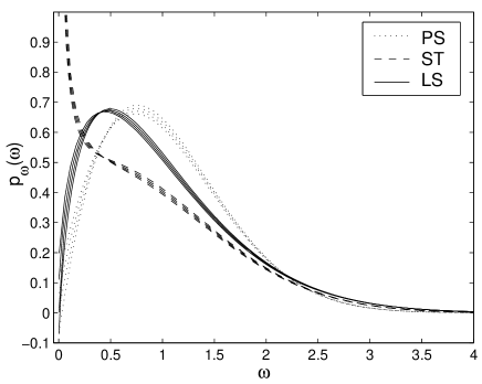
In comparing the results of PS, ST and LS in figure 5, we see that the $p_{\omega}(\omega)$ of non-spherical-collapse models (ST and LS) have larger tails at high $\omega$, allowing clusters to form at earlier time. This is consistent with the argument that in non-spherical-collapse models, halos are considered formed as long as one of three major axes has collapsed, leading to the earlier formation of clusters. This earlier formation of clusters consumes more over-density regions at early time than in the PS formalism, so as to cause the delay of the active formation epoch, i.e. the maximum of $p_{\omega}(\omega)$ being located at a lower $\omega$ (see the solid and dashed lines in figure 5). We also note that the dramatic increase of $p_{\omega}(\omega)$ towards $\omega=0$ in the ST model is nearly divergent, and this is caused by the mathematical form of $F_{\rm ST}$.

To implement all the analysis properly, we shall use the numerical result of equation (35) based on the inflationary models (invoking eq. [16]). The value of $f$ we shall use is [Viana & Liddle 1999, Navarro, Frenk & White 1995] (at $95$% confidence interval)

$$f=0.75\pm 0.15.$$ (40)

Thus the present number density of clusters of present mass $M$ that were formed at red-shift $z$ can now be obtained as $n_{i}(M,0)p_{z}(z){\rm d}M{\rm d}z$.

5 Mass-temperature relation and X-ray cluster abundance

We then need to associate the abundance $n_{i}(M,0)p_{z}(z){\rm d}M{\rm d}z$ with the temperature that corresponds the given $M$ and $z$. This requires the knowledge about the relation between the virial mass $M\equiv M_{\rm v}$ of a formation red-shift $z$ and its present temperature $T$. Here we shall use the result of Viana & Liddle (1996, 1999), which was calibrated to the hydrodynamical $N$-body simulations of White et al. (1993b), and also shown to agree well with the result by Bryan & Norman (1998). Their result of the $M$-$T$ relation is (modified from Viana & Liddle 1999):

$$\begin{array}[]{l}M_{\rm v}=(1.23\pm 0.33)\times 10^{15}\left[\frac{\Omega_{\rm mt}^{b(\Omega_{\rm mt})}}{\Omega_{\rm m}^{0}}\right]^{1/2}\left[\frac{1.67}{1+z_{\rm t}}\times\right.\\ ~{}~{}~{}~{}~{}~{}~{}~{}~{}\left.{2(2-\eta)(4-\eta)^{2}\over 64-56\eta+24\eta^{2}-7\eta^{3}+\eta^{4}}\frac{k_{\rm B}T}{7.5{\rm keV}}\right]^{3/2}h^{-1}{\rm M}_{\odot},\end{array}$$ (41)

where the error is 1-sigma, $z_{\rm t}$ is the turnaround red-shift, $\Omega_{\rm mt}\equiv\Omega_{\rm m}(z_{\rm t})$, and

$$\eta \equiv \eta(z_{\rm t})=\frac{32}{9\pi^{2}}\frac{\Omega_{\Lambda}^{0}\Omega_{\rm mt}^{b(\Omega_{\rm mt})}}{\Omega_{\rm m}^{0}(1+z_{\rm t})^{3}},$$ (42)

$$b(\Omega) = \left\{\begin{array}[]{ll}0.76-0.25\Omega&({\rm OCDM}),\\ 0.73-0.23\Omega&({\rm\Lambda CDM}).\end{array}\right.$$ (45)

For a given red-shift $z\equiv z_{\rm c}$ of cluster collapse, the turnaround red-shift $z_{\rm t}$ is easily obtained using the fact that $2t(z_{\rm t})=t(z_{\rm c})$, where

$$t(z)=\cases{\frac{2}{3}H_{0}^{-1}(1+z)^{-3/2}\quad\textrm{for $\Omega_{\rm m0}=1$, $\Omega_{\Lambda 0}=0$},\cr\frac{H_{0}^{-1}\Omega_{\rm m0}}{2(1-\Omega_{\rm m0})^{3/2}}\left[\frac{2(1-\Omega_{\rm m0})^{1/2}(1+z\Omega_{\rm m0})^{1/2}}{\Omega_{\rm m0}(1+z)}\right.\cr\left.-\cosh^{-1}\left(\frac{z\Omega_{\rm m0}-\Omega_{\rm m0}+2}{z\Omega_{\rm m0}+\Omega_{\rm m0}}\right)\right]\quad\textrm{for OCDM},\cr\frac{2H_{0}^{-1}}{3\Omega_{\Lambda 0}^{1/2}}\ln\left\{\frac{\Omega_{\Lambda 0}^{1/2}+[\Omega_{\Lambda 0}+\Omega_{\rm m0}(1+z)^{3}]^{1/2}}{\Omega_{\rm m0}^{1/2}(1+z)^{3/2}}\right\}\;\textrm{for $\Lambda$CDM}.\cr}$$ (46)

We note that although other work of the $M$-$T$ relation may suggest a different normalization from the one used in equation (41), the error quoted here should have reasonably included the possible deviations. For example, the normalization used by Pierpaoli, Scott & White (2000) is about 15% lower than here, and this is well within our 1-sigma, which is about 27% of the central value. In addition, we shall also investigate the dependence of our final result on this, so that one can easily extrapolate our final result for different $M$-$T$ normalization (see section 6.2).

Putting all the above results together, we can now estimate the present number density of galaxy clusters that were formed at a given red-shift $z$ with a mean X-ray temperature $k_{\rm B}T$:

$$\hat{n}_{i}(T,z){\rm d}(k_{\rm B}T){\rm d}z=n_{i}(M,0)p_{z}(z)\frac{3M}{2k_{\rm B}T}{\rm d}(k_{\rm B}T){\rm d}z,$$ (47)

where we have used the fact that ${\partial M}/{\partial(k_{\rm B}T)}={3M}/{2k_{\rm B}T}$. By integrating this over the temperature $T$ and the formation redshift $z\equiv z_{\rm c}$, we obtain the theoretically predicted abundance of X-ray clusters observed at $z_{\rm obs}$ with a temperature greater than a given threshold $T_{\rm th}$:

$$N_{\rm thy}(>T_{\rm th},z_{\rm obs})=\int_{0}^{\infty}\int_{k_{\rm B}T_{\rm th}}^{\infty}\hat{n}_{i}(T,z){\rm d}(k_{\rm B}T){\rm d}z.$$ (48)

We note that the $z_{\rm obs}$ on the left hand side means completely differently from the $z$ on the right hand side. The former means the red-shift of the observed clusters, while the latter means the formation red-shift of those clusters relative to $z_{\rm obs}$. Thus we need to integrate the above equation as if we were placed at $z_{\rm obs}$, i.e. we need to first shift all relevant physical conditions today ($\Omega_{\rm m0}$, $\Omega_{\rm\Lambda 0}$, etc.) to the epoch $z_{\rm obs}$ ($\Omega_{\rm m}(z_{\rm obs})$, $\Omega_{\rm\Lambda}(z_{\rm obs})$, etc.), and then integrate equation (48) as if $z_{\rm obs}=0$.

A comparison between the observed cluster abundance and the above theoretical prediction will give us an estimate of $\sigma_{8}$. The observed cluster abundance we shall use for this comparison is that given by Viana & Liddle [Viana & Liddle 1999], based on the dataset in Henry & Arnaud [Henry 1991], and updated by Henry [Henry 2000]. It is an abundance at $z_{\rm obs}=0.05$ with X-ray temperature exceeding $6.2{\rm keV}$:

$$N_{\rm obs}(>6.2{\rm keV},0.05)=1.53\times 10^{-7\pm 0.16}h^{3}{\rm Mpc}^{-3}.$$ (49)

The uncertainty in (49) is the 1-sigma interval, and has taken into account the effect of temperature measurement errors. The reasons for concentrating on galaxy clusters with temperature larger than $6.2{\rm keV}$ has been extensively discussed by Viana & Liddle [Viana & Liddle 1999].

6 Results and discussion

6.1 The $\sigma_{8}$

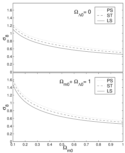
By comparing the observed cluster abundance (49) with the theoretical prediction (48), we obtained the values of $\sigma_{8}$ based on different models of mass function. Figure 6 shows the results as functions of $\Omega_{\rm m0}$ and $\Omega_{\Lambda 0}$. These results can be fitted by

$$\sigma_{8(i)}(\Omega_{\rm m0},\Omega_{\Lambda 0})=c_{1}\Omega_{\rm m0}^{\alpha},\textrm{ $i=$PS, ST, LS, and ST+LS},$$ (50)

where

$$\alpha\equiv\alpha(\Omega_{\rm m0},\Omega_{\Lambda 0})=-0.3-0.17\Omega_{\rm m0}^{c_{2}}-0.13\Omega_{\Lambda 0},$$ (51)

and the values of $c_{1}$ and $c_{2}$ are given in table 2. These fits are accurate within 2% error for $1\geq\Omega_{\rm m0}\geq 0.1$. We notice that these results of $\sigma_{8}$ have only simple dependence on $\Omega_{\Lambda}$ (the last term of eq. [51]), and this dependence is independent on the choice of mass function. It is clear that for a given $\Omega_{\rm m0}$, the cosmological constant tends to increase the normalization of $\sigma_{8}$. Also given in equation (50) and table 2 is the mean of the ST and LS results, labeled as ‘ST+LS’ (see next section for more details). It is plotted as the thick solid line in figure 7, and we shall refer to this as the combined result of non-spherical-collapse models.

Figure 6: The cluster-abundance-normalized $\sigma_{8}$ based on different mass functions. The upper and lower panels show the results in the OCDM and $\Lambda$CDM models respectively.

$i$	PS	ST	LS	ST+LS
$c_{1}$	0.54	0.50	0.455	0.477
$c_{2}$	0.45	0.37	0.31	0.34

Table 2: Values in the fit (50) of $\sigma_{8}$, based on different models of mass function.

Figure 6 indicates that the $\sigma_{8\rm(ST)}$ and $\sigma_{8\rm(LS)}$ are systematically lower than $\sigma_{8\rm(PS)}$. On average within the ranges of $\Omega_{\rm m0}$ and $\Omega_{\Lambda 0}$ probed here, we found that $\sigma_{8\rm(ST)}$ is 7% and $\sigma_{8\rm(LS)}$ is 15% smaller than $\sigma_{8\rm(PS)}$. In figure 7, we also see that the combined non-spherical-collapse results $\sigma_{8\rm(ST+LS)}$ (thick solid lines) are on average 11% lower than $\sigma_{8\rm(PS)}$ (thick dashed lines). This implies that the inclusion of non-spherical collapse considerably reduces the amplitude of mass perturbations required for resembling the observed cluster abundance. This can be understood as the consequence of the higher abundance of massive clusters in the non-spherical-collapse models. In figure 4, we saw that the non-spherical-collapse models (ST and ST) predict more massive clusters. Adding the fact that clusters are relatively rare objects that exist only with high mass, we know that the amplitude of matter perturbations required to resemble the observed cluster abundance will be lower in non-spherical-collapse models, resulting in the lower $\sigma_{8}$ as seen in figures 6 and 7.

Figure 7: The cluster-abundance-normalized $\sigma_{8}$ based on ST+LS (thick solid lines) and PS (thick dashed lines), compared with results of Viana & Liddle (1999; VL, thin solid), Eke, Cole & Frenk (1996; ECF, thin dashed), Wang & Steinhardt (1998; WS, dot-dashed), Borgani et al. (1999; B, dotted), and Pierpaoli, Scott & White (2000; PSW, circles in the lower panel), in the OCDM (upper panel) and $\Lambda$CDM (lower panel) models. The shaded areas are the 1-sigma regions of the ST+LS result. The crosses are the observational constraints derived by Henry (2000).

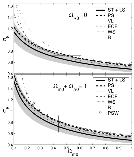
In figure 7, we have also plotted other results in the literature for comparison. They are results by Viana & Liddle (1999; VL, thin solid lines), by Eke, Cole & Frenk (1996; ECF, thin dashed lines), by Wang & Steinhardt (1998; WS, dot-dashed lines), by Borgani et al. (1999; B, dotted lines), and by Pierpaoli, Scott & White (2000; PSW, circles in the lower panel). All these results were based on the PS formalism except for the last one (PSW), which was based on the ST mass function. We see that for $\Omega_{\rm m0}>0.2$, our $\sigma_{8\rm(PS)}$ is consistent well within 10% error with all the PS-based results except for the Borgani et al. (1999) in open models. In particular, our $\sigma_{8\rm(PS)}$ is consistent with that of VL within 5% error. Since our PS framework is parallel to that of VL, we verified that this small deviation is partly caused by the fact that we used the inflationary CDM model to calculate $p_{z}(z)$ (the probability that a cluster of given mass was formed at $z$), while VL used the $p_{z}(z)$ based on a power-law-spectrum model with $n_{\rm s}=0$ (i.e., our eq. [39]). On the other hand, for non-spherical-collapse models, our $\sigma_{8\rm(ST+LS)}$ is lower than that of PSW. This discrepancy is mainly caused by the fact that we integrated the abundance over the formation shift while the PSW did not. We verified that the ignorance of the integration over the formation shift will result in a significant overestimate of $\sigma_{8}$, especially for low $\Omega_{\rm m0}$ cosmologies. This is because clusters of the same mass but formed in the past will have higher temperature and thus more observable than those formed today, so that the required $\sigma_{8}$ to resemble the observation in models allowing clusters to form in the past will be lower. We also note that our normalization for the $M$-$T$ relation is higher than that of the PSW. If we adopt their normalization, our $\sigma_{8\rm(ST+LS)}$ will be even lowered by about 5%. Overall, it is clear that our $\sigma_{8\rm(ST+LS)}$ is lower than any previous results, and this is mainly attributed to the inclusion of non-spherical collapse in our formalism.

It should be also noticed that in Henry (2000), the maximum likelihood fits of cluster evolution models to the observed cluster X-ray temperatures gave $\Omega_{\rm m0}=0.49\pm 0.12$ and $\sigma_{8}=0.72\pm 0.1$ for OCDM, and $\Omega_{\rm m0}=0.44\pm 0.12$ and $\sigma_{8}=0.77\pm 0.15$ for $\Lambda$CDM, all at 68 per cent confidence level. These results are plotted as the crosses in figure 7. They are consistent with all the results presented here.

6.2 Uncertainties

To know how stringent our results of $\sigma_{8}$ are, we investigate the dependence of $\sigma_{8}$ on $M_{\rm v}$, $f$, $N\equiv N_{\rm obs}(>6.2{\rm keV},0.05)$ and $\Gamma^{\prime}$, because they carry uncertainties in our analysis pipeline. Empirically we found

$$\frac{\sigma_{8}(\Gamma^{\prime},f,M_{\rm v},N)}{\sigma_{8}(\Gamma^{\prime}_{(0)},f_{(0)},M_{\rm v(0)},N_{(0)})}=\left(\frac{\Gamma^{\prime}}{\Gamma^{\prime}_{(0)}}\right)^{p_{\Gamma}}\left(\frac{f}{f_{(0)}}\right)^{p_{f}}\times$$

$$\left(\frac{M_{\rm v}}{M_{\rm v(0)}}\right)^{p_{M}}\left(\frac{N+\tilde{N}}{N_{(0)}+\tilde{N}}\right)^{p_{N}},$$ (52)

where the subscript $(0)$ denotes the central values (see eqs. [12], [40], [41], and [49]) that were used to obtain the main result (50), and

$$p_{\Gamma^{\prime}} = 0.14-0.13\Omega_{\rm m0}^{0.9}+0.1\Omega_{\Lambda 0}^{2},$$ (53)

$$p_{f} = 1.95-1.9\Omega_{\rm m0}^{0.12}-0.25\Omega_{\Lambda 0},$$ (54)

$$p_{M} = 0.41-0.06\Omega_{\rm m0}+0.08\Omega_{\Lambda 0},$$ (55)

$$p_{N} = 0.12\Omega_{\rm m0}^{-0.15}+0.05\Omega_{\Lambda 0}^{2}-\delta_{\rm PS}0.021\Omega_{\rm m0}^{-0.24},$$ (56)

$$\tilde{N} = 5\times 10^{-8}h^{3}{\rm Mpc}^{-3},$$ (57)

with $\delta_{\rm PS}$ equal unity for the PS, and zero otherwise. Equation (52) is accurate within $3\%$, $3\%$, $2\%$, and $0.5\%$ errors for

$$1.8> \frac{M_{\rm v}}{M_{\rm v(0)}} >0.2,$$ (58)

$$0.9> f >0.53,$$ (59)

$$3> \frac{N}{N_{(0)}} >0.3,$$ (60)

$$0.28> \Gamma^{\prime} >0.17.$$ (61)

From equation (52), we first note that within the parameter range probed here ($1\geq\Omega_{\rm m0}\geq 0.1$ and $\Omega_{\Lambda 0}=1-\Omega_{\rm m0}$ or $0$), the $\sigma_{8}$ is always a monotonically increasing function of all $M_{\rm v}$, $N$, $f$ and $\Gamma^{\prime}$. Second, it can be also inferred that within the $68\%$ confidence level of $M_{\rm v}$, $N$, $f$ and $\Gamma^{\prime}$ (see eqs. [41], [49], [40], and [12]), the resulting $\sigma_{8}$ within the parameter range probed here can vary up to $14\%$, $6\%$, $5\%$, and $2\%$ respectively, depending on the background cosmology. Thus we see that an improvement in reducing the uncertainty in $M_{\rm v}$, the normalization of the $M$-$T$ relation, can most efficiently reduce the uncertainty in the resulting $\sigma_{8}$. To the contrary, a more accurate estimation of the degenerated shape parameter $\Gamma^{\prime}$ will not change the resulting $\sigma_{8}$ much. This observation helps relax the worry about the accuracy in using the parameterization (10), and the approximation (6), which we have used to model baryonic effects.

To investigate the overall uncertainties in $\sigma_{8}$ (that is, to include the uncertainties from all $M_{\rm v}$, $f$, $N$ and $\Gamma^{\prime}$ simultaneously), we implemented Monte Carlo simulations, with the distributions of the uncertainties in $\Gamma^{\prime}$ and $N_{\rm obs}(>6.2{\rm keV},0.05)$ as log-normal, and those in $M_{\rm v}$ and $f$ as Gaussian (see eqs. [12], [40], [41], and [49]). We found that the distribution of the resulting $\sigma_{8}$ is very much Gaussian, with a mean given by equation (50) and table 2, and a standard deviation ($68\%$ confidence level)

$$\epsilon_{i}(\Omega_{\rm m0},\Omega_{\Lambda 0})=0.1\Omega_{\rm m0}^{-0.15}\sigma_{8(i)}(\Omega_{\rm m0},\Omega_{\Lambda 0}),\quad i=\textrm{PS, ST, LS}.$$ (62)

We have verified that this result is very weekly dependent on $\Omega_{\Lambda 0}$ and the choice of the mass function (PS, ST, or LS), and these two aspects together contribute only a deviation of less than 3% from the above result.

To obtain a single result for the non-spherical-collapse models (ST and LS), we linearly combine the probability distribution functions of $\sigma_{8\rm(ST)}$ and $\sigma_{8\rm(LS)}$ obtained from the above Monte Carlo simulations. The resulting distribution of $\sigma_{8}$ is very Gaussian. It has a mean given by equation (50) and table 2 (the ST+LS result), and a standard deviation

$$\epsilon_{\rm ST+LS}(\Omega_{\rm m0},\Omega_{\Lambda 0})=0.11\Omega_{\rm m0}^{-0.12}\sigma_{8{\rm(ST+LS)}}(\Omega_{\rm m0},\Omega_{\Lambda 0}).$$ (63)

Figure 7 shows this ST+LS result as the thick solid lines (the mean; eq. [50] and tab. 2) with shaded areas (the 1-sigma regions; eq. [63]). Also plotted for comparison is the PS result (the thick dashed lines). It is clear that the result based on non-spherical-collapse models is about one sigma lower than the PS result, due to the origin already argued in section 6.1.

In our entire analysis, we have used $\Omega_{\rm B0}=0.05$, but verified that for $0.05\geq\Omega_{\rm B0}\geq 0$, the normalization of $\sigma_{8}$ was affected by less than 1%. We have also tested that the difference between the $\sigma_{8}$ based on the $p_{z}(z)$ of the standard CDM model and of the power-law-spectrum model with $n_{\rm s}=0$ is less than 3% in all cases. In addition, we explore the effect of the integration over the formation redshift $p_{z}(z)$ based on different models of mass function, i.e. while keeping the mass function the same (PS, ST or LS), we use different $p_{z(i)}(z)$ ($i=$PS, ST or LS) to calculate $\sigma_{8}$. It is found that for a given model of mass function, the $\sigma_{8}$ is higher when using $p_{z\rm(LS)}(z)$ than using $p_{z\rm(PS)}(z)$, and is even higher when using $p_{z\rm(ST)}(z)$. Adding the fact that $p_{z\rm(ST)}(z)$ and $p_{z\rm(LS)}(z)$ have maxima located at lower $z$ than $p_{z\rm(PS)}(z)$ (see figure 5), the above result is consistent with the previously argued and verified fact that the required $\sigma_{8}$ to reproduce the observed cluster abundance will be lower if clusters are actively formed earlier (and thus have higher temperature and are more observable). Nevertheless, the difference in the $\sigma_{8}$ using different $p_{z}(z)$ but the same mass function is always less than 3%. Therefore, we conclude that the previously observed lower normalization of $\sigma_{8}$ in the non-spherical-collapse models is indeed mainly caused by the form of the mass function itself, rather than by its form of the formation-redshift probability, which in fact has opposite effect.

6.3 Redshift distortion parameter

Another important aspect in the study of large-scale structure is the so-called ‘redshift distortion parameter’. It quantifies the confusion between the Hubble flow and the peculiar velocities, and is analytically defined as [Kaiser 1987]

$$\beta_{j}(\Omega_{\rm m0},\Omega_{\Lambda 0})=\frac{f(\Omega_{\rm m0},\Omega_{\Lambda 0})}{b_{j}}=f(\Omega_{\rm m0},\Omega_{\Lambda 0})\frac{\sigma_{8}}{\sigma_{8(j)}},$$ (64)

where $b_{j}\equiv\sigma_{8(j)}/\sigma_{8}$ is the $j$-type galaxy to mass bias ($j=$IRAS, optical, etc.), and [Lahav et al. 1991]

$$f(\Omega_{\rm m0},\Omega_{\Lambda 0})\approx\Omega_{\rm m0}^{0.6}+\frac{\Omega_{\Lambda 0}}{70}(1+\frac{\Omega_{\rm m0}}{2}),$$ (65)

which is the rate of growth of matter perturbations at the present epoch. Here we shall estimate $\beta_{\rm I}$, with the subscript ‘I’ indicating the IRAS galaxies. To this end, we can substitute the result (50) (which is calibrated from cluster abundance) and the result (13) (which is obtained from the IRAS PSCz survey) into equation (64). By combining their likelihoods together, we obtained the maximum-likelihood result, which can be fitted as

$$\beta_{{\rm I}(i)}(\Omega_{\rm m0},\Omega_{\Lambda 0})=d_{1}\Omega_{\rm m0}^{d_{2}-0.16(\Omega_{\rm m0}+\Omega_{\Lambda 0})},\textrm{$i=$PS, ST+LS,}$$ (66)

where the values of $d_{1}$ and $d_{2}$ are given in table 3. This fit is accurate within 2% error. The errors at 68 per cent confidence level was also found as

$$\epsilon_{{\scriptscriptstyle\beta}(i)}(\Omega_{\rm m0},\Omega_{\Lambda 0})=0.176\Omega_{\rm m0}^{-0.11}\beta_{{\rm I}(i)}(\Omega_{\rm m0},\Omega_{\Lambda 0}).$$ (67)

This fit is accurate within 1% error. These results are plotted in figure 8.

$i$	PS	ST+LS
$d_{1}$	0.693	0.613
$d_{2}$	0.26	0.24

Table 3: Values in the fit (66) of $\beta_{{\rm I}(i)}$, based on different models of mass function.

Figure 8: Linear redshift distortion parameter $\beta_{\rm I}$, estimated from the combined maximum-likelihood analysis of $\sigma_{8{\rm(I)}}$ and $\sigma_{8}$. The solid lines are based on non-spherical-collapse models (ST+LS), with the shaded areas representing the regions within 68 per cent confidence level. The dotted lines are based on the PS formalism.

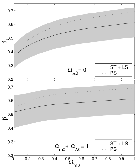
From figure 8, we first note that the $\beta_{\rm I(ST+LS)}$ is systematically lower than $\beta_{\rm I(PS)}$. This is a direct consequence of the fact that $\beta_{\rm I}\propto\sigma_{8}$, which is lower in non-spherical-collapse models as previously observed. We also see that the inclusion of the cosmological constant tends to increase $\beta_{\rm I}$. In the past, $\beta_{\rm I}$ has been measured by many authors using different observations (for a review, see Strauss & Willick 1995). The combined result of these observations has a central value of about $\beta_{\rm I}\approx 0.7$, but with a large 68 per cent confidence region of about $\pm 0.4$. In recent years, observations seem to favor a lower value. For example, $\beta_{\rm I}=0.41^{+0.13}_{-0.12}$ by Hamilton, Tegmark & Padmanabhan (2000), and $\beta_{\rm I}=0.39\pm 0.12$ by Taylor et al. (2000). If these measures are correct, then the PS-based $\beta_{\rm I(PS)}$ (dotted lines in fig. 8) will be in trouble except in the very low $\Omega_{\rm m0}$ regime, and the non-spherical-collapse models will serve to relax this situation (solid lines in fig. 8).

7 Conclusion

In this paper, we first used the observed linear mass power spectra to estimate the spectral index $n$, the shape parameter $\Gamma$, the degenerated shape parameter $\Gamma^{\prime}$, and the IRAS $\sigma_{8{\rm(I)}}$ (see table 1, eqs. [11], [13]). We then derived the probability distribution function of cluster formation redshift for different models of mass function. We found that clusters of the same mass can form earlier but have a later epoch of active formation in the non-spherical-collapse models (ST and LS) than in the PS formalism. This is consistent with the observation from numerical simulations. Based on different models of mass function and their associated probability distributions of formation redshift, we then used the observed cluster abundance to estimate the amplitude of matter density perturbations on the scale of $8h^{-1}$Mpc, $\sigma_{8}$, and the redshift distortion parameter for IRAS galaxies, $\beta_{\rm I}$, in both OCDM and $\Lambda$CDM cosmologies. The $\sigma_{8}$ and $\beta_{\rm I}$ resulted from non-spherical-collapse models are systematically lower than those based on the PS formalism. We showed that this is mainly owing to the larger mass function at the high mass end in the non-spherical-collapse models. The origins of the uncertainties in our final results were also investigated separately, and we found that the main contribution is from the uncertainty in the normalization of the virial mass-temperature relation. Therefore we expect that further improvement in the study of this normalization will provide us with more stringent constraint on both $\sigma_{8}$ and $\beta_{\rm I}$. In addition, since we saw significant corrections in the resulting $\sigma_{8}$ and $\beta_{\rm I}$ when switching from the conventional Press-Schechter formalism to the more recent non-spherical-collapse models, we urge the use of these models in all relevant studies, especially when we are entering the regime of precision cosmology.

References

- [Avelino, Wu & Shellard 2000] Avelino P. P., Wu J. H. P., Shellard E. P. S., 2000, MNRAS, 318, 329
- [Borgani et al. 1999] Borgani S., Rosati P., Tozzi P., Norman C., 1999, ApJ, 517, 40
- [Bryan & Norman 1998] Bryan G. L., Norman M. L., 1998, ApJ, 495, 80
- [Balbi et al. 2000] Balbi A. et al., 2000, ApJL in press, astro-ph/0005124
- [Carroll, Press & Turner 1992] Carroll S. M., Press W. H., Turner E. L., 1992, Annu. Rev. Astron. Astrophys., 30, 499
- [Eisenstein & Hu 1998] Eisenstein, D. J., Hu, W., 1998, ApJ, 496, 605
- [Eke, Cole & Frenk 1996] Eke V. R., Cole S., Frenk C. S., 1996, MNRAS, 282, 263
- [Hamilton, Tegmark & Padmanabhan 2000] Hamilton A. J. S., Tegmark M., Padmanabhan N., 2000, astro-ph/0004334
- [Hamilton & Tegmark 2000] Hamilton A. J. S., Tegmark M., 2000, astro-ph/0008392
- [Henry 1991] Henry J. P., Arnaud K. A., 1991, ApJ, 372, 410
- [Henry 2000] Henry J. P., 2000, ApJ, in press, astro-ph/0002365
- [Jaffe et al. 2000] Jaffe A. H. et al., 2000, PRL submitted, astro-ph/0007333
- [Kaiser 1987] Kaiser N., 1987, MNRAS, 227, 1
- [Kitayama & Suto 1997] Kitayama T., Suto Y., 1997, ApJ, 490, 557
- [Kolb & Turner 1990] Kolb E. W., Turner M. S., 1990, ‘The Early Universe’, Addison-Wesley, Redwood City, California
- [Lacey & Cole 1993] Lacey C., Cole S., 1993, MNRAS, 262, 627
- [Lacey & Cole 1994] Lacey C., Cole S., 1994, MNRAS, 271, 676
- [Lahav et al. 1991] Lahav O., Lilje P. B., Primack J. R., Rees M. J., 1991, MNRAS, 251, 128
- [Lange et al. 2000] Lange A. E. et al., 2000, PRD submitted, astro-ph/0005004
- [Lee & Shandarin 1998] Lee J., Shandarin S. F., 1999, ApJ, 500, 14
- [Lee & Shandarin 1999] Lee J., Shandarin S. F., 1999, ApJ, 517, L5
- [Navarro, Frenk & White 1995] Navarro J. F., Frenk C. S., White S. D. M., 1995, MNRAS, 275, 720
- [Peacock & Dodds 1994] Peacock J. A., Dodds S. J., 1994, MNRAS, 267, 1020
- [Pierpaoli, Scott & White 2000] Pierpaoli E., Scott D., White M., 2000, astro-ph/0010039
- [Press & Schechter 1974] Press W. H., Schechter P., 1974, ApJ, 187, 452
- [Saunders et al. 2000] Saunders W., Sutherland W. J., Maddox S.. J., Keeble O., Oliver S. J., Rowan-Robinson M., McMahon R. G., Efstathiou G. P., Tadros H., White S. D. M., Frenk C. S., Carraminana A., Hawkings M. R. S., 2000, MNRAS submitted, astro-ph/0001117 (PSCz, available at http://www-astro.physics.ox.ac.uk/ wjs/pscz.html)
- [Sheth & Tormen 1999] Sheth R. K., Tormen G., 1999, MNRAS, 308, 119
- [Sheth, Mo & Tormen 1999] Sheth R. K., Mo H. J., Tormen G., 1999, astro-ph/9907024
- [Strauss & Willick 1995] Strauss M. A., Willick J., 1995, Phys. Rep., 261, 271
- [Sugiyama 1995] Sugiyama, N., 1995, ApJS, 100, 281
- [Taylor et al. 2000] Taylor A. N., Ballinger W. E., Heavens A. F., Tadros H., 2000, astro-ph/0007048
- [Tormen 1998] Tormen G., 1998, MNRAS, 297, 648
- [Viana & Liddle 1996] Viana P. T. P., Liddle A. R., 1996, MNRAS, 281, 323
- [Viana & Liddle 1999] Viana P. T. P., Liddle A. R., 1999, MNRAS, 303, 535
- [Wang & Steinhardt 1998] Wang L., Steinhardt P. J., 1998, ApJ, 508, 483
- [White, Efstathiou & Frenk 1993a] White S. D. M., Efstathiou G., Frenk C. S., 1993a, MNRAS, 262, 1023
- [White, Navarro, Evrard & Frenk 1993b] White S. D. M., Navarro J. F., Evrard A. E., Frenk C. S., 1993b, Nat, 366, 429