Cluster Mass Profiles from Weak Lensing II

Abstract

When a cluster gravitationally lenses faint background galaxies, its tidal gravitational field distorts their shapes (shear effect) and its magnification effect changes the observed number density. In Schneider, King & Erben (2000) we developed likelihood techniques to compare the constraints on cluster mass profiles that can be obtained using the shear and magnification information. This work considered circularly symmetric power-law models for clusters at fairly low redshifts where the redshift distribution of source galaxies could be neglected. Here this treatment is extended to encompass NFW profiles which are a good description of clusters from cosmological N-body simulations, and NFW clusters at higher redshifts where the influence of various scenarios for the knowledge of the redshift distribution are examined. Since in reality the overwhelming majority of clusters have ellipsoidal rather than spherical profiles, the singular isothermal ellipsoid (SIE) is investigated. We also briefly consider the impact of substructure on such a likelihood analysis.

In general, we find that the shear information provides a better constraint on the NFW profile under consideration, so this becomes the focus of what follows. The ability to differentiate between the NFW and power-law profiles strongly depends on the size of the data field, and on the number density of galaxies for which an ellipticity can be measured. Combining Monte Carlo simulations with likelihood techniques is a very suitable way to predict whether profiles will be distinguishable, given the field of view and depth of the observations.

For higher redshift NFW profiles, there is very little reduction $(\sim 1.5\%)$ in the dispersion of parameter estimates when spectroscopic redshifts, as opposed to photometric redshift estimates, are available for the galaxies used in the lensing analysis.

1 Introduction

Gravitational lensing provides an invaluable means to investigate how luminous and dark matter is distributed in the Universe, from inside our own Galaxy to cosmological scales [e.g. Alcock (2000), Keeton et al. (1998), van Waerbeke et al. (2000)]. In this paper we focus on clusters in the weak lensing regime, where the number density and shapes of faint background galaxies are changed through the magnification and shear effects respectively. These signatures can be used to determine the projected mass distribution of the lensing cluster.

The pioneering work of Kaiser & Squires (1993) describes how to obtain a parameter-free reconstruction of a mass distribution, and this technique has been applied to many clusters [e.g. Fischer & Tyson 1997; Clowe et al. 1998; Hoekstra et al. 1998; Clowe et al. 2000; Hoekstra, Franx & Kuijken 2000]. In contrast to parameterised models, the interpretation of such mass maps is difficult since the error properties of non-parametric models are poorly understood. Although deriving parameterised cluster models from weak lensing data may not reveal the lensing mass distribution in the same detail, it enables different families of models to be explored, and statistical comparisons between clusters to be made.

In Schneider, King & Erben (2000; hereafter SKE) we investigated parameterised cluster models and developed likelihood techniques to quantify the accuracy with which parameters can be recovered using the magnification and shear information. Two simple but generic families of power-law models for the surface mass density were studied. The basic model has a monotonically decreasing form, and is defined outside the Einstein radius ($\theta_{{\rm E}}$), which marks the transition between the weak and strong lensing regimes.

Here we extend this work to encompass two other parameterised lens models that are commonly used to describe cluster mass profiles: the NFW profile (Navarro, Frenk & White 1996;1997), and the singular isothermal ellipsoid (SIE) as discussed by Kormann, Schneider & Bartelmann (1994). The impetus for considering the NFW profile is that it is a good description of the radial density profiles of virialised dark matter halos formed in cosmological simulations of hierarchical clustering. The SIE model allows us to investigate non-spherically symmetric dark matter distributions. The influence of uncertainty in the redshift distribution of galaxies used in the lensing analysis is examined, in the context of NFW clusters at higher redshifts.

A question of fundamental importance to the study of galaxy and cluster formation, and to the nature of dark matter itself, is how profiles can best be described [e.g. Moore et al. 2000]. Therefore, we investigate whether we can distinguish between NFW and power-law models, and the constraints that can be placed on SIE models.

We also briefly address the influence of substructure on our analysis, by comparing the smooth NFW profile with a toy model containing substructure.

The structure of this paper is as follows: the notation and lensing relationships used are outlined in Section 2, followed by the basis of using the magnification and shear methods in constraining a cluster mass profile. In Section 3, the likelihood functions developed in SKE are briefly presented. Moving to clusters at higher redshifts, several scenarios for our knowledge of the source redshift distribution are described. Monte Carlo simulations were performed in order to check the validity of the analytic treatment, and to deal with cases where the redshift distribution is important; a prescription for these is given in Section 4. The relevant properties of the lens models considered in this work are also given in this Section.

The results from the likelihood analysis in the case of lower redshift clusters are presented in Section 5. For the NFW profile, proceeding as in SKE, we check the validity of the assumption of $\chi^{2}$ statistics. Also, a brief comparison is made between the accuracy of parameters recovered using the magnification and shear information. Then the shear method becomes the focus and we ask whether it is possible to distinguish between the NFW and other profiles, using our likelihood analysis. Moving to the SIE model, we want to ascertain how well the axial ratio of a mass distribution is recovered – can we detect deviation from circular symmetry and put constraints on the position angle of the lens model? The results for NFW clusters at higher redshifts, for different degrees of source redshift information, are presented in Section 6. Lastly, we consider what effect adding substructure to the smooth NFW model has on our analysis. In the final Section we summarise our conclusions.

2 Shear and magnification methods

In this Section the notation used throughout this paper is introduced, along with the basic definitions and relationships. Then the methods for constraining the mass profile of a lens using the shape distortions and the change in the number density of background galaxies are outlined.

2.1 Notation, basic definitions and relationships

Throughout, standard lensing notation is used [eg Schneider, Ehlers & Falco 1992; Bartelmann & Schneider (2000)].

The surface mass density of a lens at position $\@vec{\theta}$ is denoted by $\Sigma(\@vec{\theta})$ and the critical surface mass density of a lens at redshift $z_{\rm d}$ for sources at redshift $z$ by $\Sigma_{\rm crit}(z)\equiv\frac{c^{2}}{4\pi G}\frac{D_{{\rm s}}}{D_{{\rm d}}D_{{\rm d}{\rm s}}}$, where $D_{{\rm s}},D_{{\rm d}},D_{{\rm d}{\rm s}}$ are the observer–source, observer–lens and lens–source angular diameter distances respectively. The dimensionless surface mass density of a lens, $\kappa(\@vec{\theta},z)$, is the ratio of $\Sigma/\Sigma_{\rm crit}$, and a Poisson-like equation relates the deflection potential $\psi(\@vec{\theta})$ to $\kappa$

$$\nabla^{2}\psi=2\kappa\;.$$ (1)

The complex shear is a combination of second derivatives of the potential

$$\gamma=\gamma_{1}+{\rm i}\gamma_{2}=(\psi_{11}-\psi_{22})/2+{\rm i}\psi_{12}$$ (2)

(the subscript indices denote partial derivatives with respect to the position $\@vec{\theta}$ on the sky). Further, $g=\gamma/(1-\kappa)$ is the complex reduced shear. The magnification of an image is the inverse of the Jacobian determinant of the lens equation,

$$\mu(\@vec{\theta})=[\det{\cal A}(\@vec{\theta})]^{-1};\leavevmode\nobreak\ \leavevmode\nobreak\ \leavevmode\nobreak\ \leavevmode\nobreak\ \det{\cal A}=(1-\kappa)^{2}-|\gamma|^{2}\;.$$ (3)

In Section 4 the expressions specific to the lens model families considered here are given.

The strength of a lens depends on the relative redshifts of the observer, lens and source, and as in Seitz & Schneider (1997) it is convenient to introduce a redshift dependent lensing strength factor $w(z)$. Then we can express $\kappa(z)=w(z)\kappa_{\infty}$ and $\gamma(z)=w(z)\gamma_{\infty}$, where $\kappa_{\infty}$ and $\gamma_{\infty}$ correspond to quantities at position $\@vec{\theta}$ for hypothetical sources located at $z=\infty$. In the Einstein-de Sitter $\Omega=1,\Lambda=0$ cosmology which we adopt,

$$w(z)=\frac{\sqrt{1+z}-\sqrt{1+z_{{\rm d}}}}{\sqrt{1+z}-1}\leavevmode\nobreak\ ;\leavevmode\nobreak\ \leavevmode\nobreak\ z>z_{{\rm d}}$$ (4)

– of course, $w(z)=0$ when $z<z_{{\rm d}}$ since the source is not lensed. It follows that $g$ and $\mu$ can be written as

$$g(\theta,z)=\frac{w(z)\gamma_{\infty}}{1-w(z)\kappa_{\infty}}$$ (5)

and

$$\mu(\theta,z)=\frac{1}{[1-w(z)\kappa_{\infty}]^{2}-[w(z)\gamma_{\infty}]^{2}}$$ (6)

respectively. In SKE we considered the case of fairly low redshift clusters where $w(z)$ is nearly constant for most galaxies used in the lensing analysis, and the differential probability distribution $p(w){{\rm d}}w$ (equivalent to $p(z){{\rm d}}z$) is a very narrow distribution. Then, the redshift distribution of the source galaxy population can safely be neglected, approximating them to be located at a redshift corresponding to the mean value of $w(z)$. If the cluster is at a higher redshift, $\mathrel{\mathchoice{\lower 2.0pt\vbox{\halign{$\m@th\displaystyle\hfil#\hfil$\cr>\crcr\sim\crcr}}}{\lower 2.0pt\vbox{\halign{$\m@th\textstyle\hfil#\hfil$\cr>\crcr\sim\crcr}}}{\lower 2.0pt\vbox{\halign{$\m@th\scriptstyle\hfil#\hfil$\cr>\crcr\sim\crcr}}}{\lower 2.0pt\vbox{\halign{$\m@th\scriptscriptstyle\hfil#\hfil$\cr>\crcr\sim\crcr}}}}0.25$ say, then the redshift distribution of the galaxies becomes important and this sheet approximation is no longer robust (Bartelmann & Schneider 2000).

Throughout, we take $H_{0}=65\leavevmode\nobreak\ {\rm km\leavevmode\nobreak\ s}^{-1}{\rm Mpc}^{-1}$.

2.2 The basis of the magnification and shear methods

2.2.1 Shear method

The galaxy ellipticity ${\epsilon}$ is defined by a complex number whose modulus is $|{\epsilon}|=(1-r)/(1+r)$, in the case of elliptical isophotes with axis ratio $r\leq 1$, and whose phase is twice the position angle of the major axis. A Gaussian probability distribution with dispersion $\sigma_{{\epsilon}^{s}}$ is adopted for the ellipticity

$$p_{\epsilon^{{\rm s}}}=\frac{\exp\left(-|{\epsilon}^{{\rm s}}|^{2}/\sigma_{{\epsilon}^{{\rm s}}}^{2}\right)}{\pi\sigma^{2}_{{\epsilon}^{{\rm s}}}\left[1-\exp\left(-1/\sigma_{{\epsilon}^{{\rm s}}}^{2}\right)\right]}\;.$$ (7)

A transformation relates the source (${\epsilon}^{{\rm s}}$) and image (${\epsilon}$) ellipticities, which are changed by the tidal gravitational field of the lens. We focus on the non-critical regime (det ${\cal A}>0$) where

$${\epsilon}={{\epsilon}^{{\rm s}}+g\over 1+g^{*}{\epsilon}^{{\rm s}}}\;.$$ (8)

The lensed and unlensed probability distributions are related through

$$p_{\epsilon}=p_{{\epsilon}^{{\rm s}}}\left|\frac{{\rm d^{2}\epsilon^{{\rm s}}}}{{\rm d^{2}{\epsilon}}}\right|\;,$$ (9)

when the distribution in source redshift is unimportant [see Eq.(19) for the more general form].

It can be shown that the expectation value for the lensed ellipticity $\left\langle{\epsilon}\right\rangle=g$ in the non-critical regime (e.g. Schramm & Kayser 1995), and that $\left\langle{\epsilon}\right\rangle=1/g^{*}$ in the critical regime (Seitz & Schneider 1997). This is the basis of the using the distorted images of background galaxies to constrain the cluster model.

2.2.2 Magnification method

The magnification method is based on the change in the local number counts of background galaxies by the magnification bias (e.g. Canizares 1982). The local cumulative number counts $n(\@vec{\theta};S)$ above flux limit $S$ are related to the unlensed counts $n_{0}(S)$ by

$$n(\@vec{\theta};S)={1\over\mu}n_{0}\,\left(S\over\mu\right)\;.$$ (10)

If we assume that the number counts locally follow a power law of the form $n_{0}\propto S^{-\beta}$, then

$$n(\@vec{\theta})=n_{0}\,\mu(\@vec{\theta})^{\beta-1}$$ (11)

at any fixed flux threshold. This implies that if the intrinsic counts are flatter than $1$, then the lensed counts will be reduced relative to the unlensed ones.

3 Likelihood treatment

The goal of our likelihood treatment is to obtain the best-fitting parameters and their error estimates for simulated or real observations [see for example Press et al. (1992)]. Generally, it is more sensible computationally to minimise log-likelihood functions to obtain the best-fitting parameters, since a large number of galaxies is involved. Whereas a log-likelihood function pertains to a single data set or realisation, ensemble averaged log-likelihood functions represent the average over many such realisations, and enable the characteristic (expected) errors associated with the recovered parameters to be estimated.

We consider cluster lenses described by parameterised models, with true parameters $\pi_{{\rm t}}$, best-fit parameters $\pi_{\rm max}$, and trial parameters (en route to minimisation) $\pi$ throughout. Quantities that refer to the true model value are subscripted with a “t”, and those referring to observed values are subscripted with an “$i$”. We assume that in an aperture centred on the cluster there are $N_{\mu}$ images of background galaxies at positions $\@vec{\theta}_{i}$, above a given flux limit, and $N_{\gamma}$ images at positions $\@vec{{\vartheta}}_{i}$ for which an ellipticity can be measured. There can be an overlap between the two sets of galaxies.

3.1 Likelihood functions

Here the expressions for the likelihood functions and ensemble averaged log-likelihood functions are reproduced; the reader is referred to SKE for the details and derivations. Minimising these functions gives $\pi_{\rm max}$, the most likely parameters given the observations. In the absence of a redshift distribution for the background sources, the magnification log-likelihood function is

$$\ell_{\mu}=n_{\mu}\int{\rm d}^{2}\theta[\mu(\@vec{\theta})]^{\beta-1}+(1-\beta)\sum_{i=1}^{N_{\mu}}{\rm\ln\;}\mu(\@vec{\theta}_{i})\;.$$ (12)

The noise in the magnification method is due to Poisson noise on the number of galaxies in the aperture. The first term in Eq.(12) dominates the expression, and gives the number of galaxies expected in the aperture, given $\pi$. Given this number of galaxies, the second term depends on how they are distributed. One noteworthy caveat of the magnification method that we uncovered in SKE is that it requires accurate knowledge of the unlensed number density, $n_{\mu}$.

The shear log-likelihood function is

$$\ell_{\gamma}=-\sum_{i=1}^{N_{\gamma}}{\rm\ln\;}p_{\epsilon}(\epsilon_{i}|g(\@vec{{\vartheta}}_{i}))\;,$$ (13)

and the noise in this method arises from the intrinsic dispersion in the galaxy ellipticity distribution, $\sigma_{{\epsilon}^{{\rm s}}}$. Eq.(13) just depends on how probable particular lensed ellipticities are, given the $\pi$ under consideration. Unlike the magnification method, the shear method does not require that the unlensed number density is accurately known.

Eq.(13) can be used numerically with the exact probability distribution for $p_{{\epsilon}}$, but for analytic work the log-likelihood function $\ell_{\gamma}$ can be dealt with as

$$\ell_{\gamma}=\sum_{i=1}^{N_{\gamma}}\frac{({\epsilon}_{i}-g(\@vec{{\vartheta}}_{i}))^{2}}{\sigma_{{\epsilon}}^{2}(g(\@vec{{\vartheta}}_{i}))}+2\ln\sigma_{{\epsilon}}(g(\@vec{{\vartheta}}_{i}))\;,$$ (14)

where $\sigma_{{\epsilon}}\approx(1-|g|^{2})\sigma_{{\epsilon}^{s}}$. For $|g|\leq 1.0$, this approximation is accurate to $\approx 5\%$ when $\sigma_{{\epsilon}}=0.2$.

The combined shear and magnification log-likelihood is obtained by adding the respective log-likelihoods:

$$\ell_{\rm tot}=\ell_{\mu}+\ell_{\gamma}\;.$$ (15)

As mentioned above, the ensemble averaged log-likelihood functions allow the characteristic errors for parameters to be derived. The ensemble averaged log-likelihood function for the magnification is

$$\left\langle\ell_{\mu}\right\rangle = n_{\mu}\int{\rm d}^{2}\theta\;[\mu(\@vec{\theta})]^{\beta-1}$$ (16)

$$+ n_{\mu}(1-\beta)\int{\rm d}^{2}\theta\;[\mu_{{\rm t}}(\@vec{\theta})]^{\beta-1}\,\ln\mu(\@vec{\theta})\;,$$

where $\mu_{{\rm t}}(\@vec{\theta})$ is the magnification determined for $\pi_{{\rm t}}$.

For the shear we have

$$\left\langle\ell_{\gamma}\right\rangle = n_{\gamma}\int{\rm d}^{2}{\vartheta}\;[\mu_{{\rm t}}(\@vec{{\vartheta}})]^{\beta-1}$$ (17)

$$\times \left({|g(\@vec{{\vartheta}})-g_{{\rm t}}(\@vec{{\vartheta}})|^{2}+\sigma_{{\epsilon},{\rm t}}^{2}(\@vec{{\vartheta}})\over\sigma_{{\epsilon}}^{2}(\@vec{{\vartheta}})}+2\ln\sigma_{{\epsilon}}(\@vec{{\vartheta}})\right)\;,$$

where again $\mu_{{\rm t}},g_{{\rm t}}$ and $\sigma_{{\epsilon}}(g_{{\rm t}})$ are determined for $\pi_{{\rm t}}$.

We have numerically implemented the expressions for the ensemble averaged log-likelihood functions which means that for specified observing conditions (i.e. $n_{\gamma}$, $n_{\mu}$ and size of the data field) the characteristic errors on parameterised models can easily be obtained. This is helpful when assessing the benefits of current telescopes with different cameras, or future ground- or space-based instruments.

In Section 5 we demonstrate that the distribution of $2\Delta\left\langle\ell\right\rangle\equiv 2(\left\langle\ell\right\rangle_{\rm max}-\left\langle\ell\right\rangle_{{\rm t}})$ for $\pi_{\rm max}$ tends to a $\chi_{M}^{2}$ distribution, where $M$ is the number of model parameters, so that error interpretation in the framework of Gaussian distributed errors is a good approximation.

3.2 Including a redshift distribution

For clusters at intermediate and high redshifts there are several ways to proceed when obtaining best-fit parameters, depending on our knowledge of the individual background galaxy redshifts. In this Section a few scenarios for the information on the redshift distribution are briefly outlined and in Section 6 a comparison is made between the dispersion in parameters recovered under each assumption.

Let the true redshifts of the background sources, denoted by $z_{t}$, be drawn from a probability distribution $p(z){{\rm d}}z$. Here, the redshift probability distribution used to generate catalogues of lensed galaxies is taken from Brainerd et al. (1996):

$$p(z){\rm d}z=\frac{\eta z^{2}e^{-(z/z_{0})^{\eta}}}{\Gamma(\frac{3}{\eta})z_{0}^{3}}{\rm d}z\;,$$ (18)

where below it is assumed that $z_{0}=1/3$ and $\eta=1.0$, resulting in $\left\langle z\right\rangle=1.0$.

In its most general form, in the presence of a redshift distribution $p_{\epsilon}$ becomes

$$p_{\epsilon}(\epsilon|\kappa_{\infty},\gamma_{\infty}) = \int_{0}^{\infty}p_{\epsilon^{s}}\left(\epsilon^{s}\left[{\epsilon},g(z)\right]\right)\left|\frac{{\rm d^{2}\epsilon^{s}}}{{\rm d^{2}\epsilon}}\right|({\epsilon},g(z))$$ (19)

$$\times p_{z}(z){\rm d}z$$

and this is inserted into the likelihood function. Eq.(19) is very difficult to deal with analytically, as discussed by Geiger & Schneider (1998) who give some approximations for the integral.

In this work we explore a few different routes:

• For the purposes of comparison, the ideal case is where (i) all redshifts are known exactly.

• Second, we consider the situation where (ii) photometric redshift estimates $z_{\rm ph}$ are available for individual galaxies.

• A common practice in mass reconstruction is to assume that (iii) the galaxies used in the lensing analysis are at a single redshift $z_{\rm sheet}$, determined by the arithmetic mean of the weighting factor $\left\langle w\right\rangle$.

• Another computationally reasonable possibility is to assume that (iv) the form of $p(z){\rm d}z$ is known, but not the redshifts of individual sources, and to integrate (19) numerically.

The availability of photometric redshift estimates is becoming more observationally realistic [e.g. Connolly et al. 1995; Fernández-Soto, Lanzetta & Yahil 1999; Benítez 2000] and has a great impact on lensing (e.g. Dye et al. (2000)). Obviously, the smaller the dispersion $\sigma_{z}$ in $z_{\rm ph}$, the smaller the dispersion in $\pi_{\rm max}$. This can be quantified with a simple estimate: The lensed probability distribution $p_{{\epsilon}}({\epsilon})$ is convolved with the Gaussian describing the distribution of $z_{\rm ph}$ around $z_{t}$. In the weak lensing limit, $g\sim w\gamma_{\infty}$ so it is convenient to work with $w$ rather than $z$, where the dispersion in $w_{\rm ph}$ is $\sigma_{w}$. Further using $\sigma_{{\epsilon}}\sim\sigma_{{\epsilon}^{{\rm s}}}$ gives

$$p_{\epsilon}(\epsilon) = \int_{0}^{1}\frac{{\rm exp}\left(-\frac{|\epsilon-{w_{\rm ph}}\gamma_{\infty}|^{2}}{\sigma_{\epsilon^{{\rm s}}}^{2}}\right)}{\pi\sigma_{{\epsilon}^{{\rm s}}}^{2}}$$ (20)

$$\times \frac{{\rm exp}\left(-\frac{({w_{\rm ph}}-{w}_{t})^{2}}{2\sigma_{w}^{2}}\right)}{\sqrt{2\pi}\sigma_{w}}{\rm d}w_{\rm ph}\;.$$

The integration can approximately be replaced by one between $-\infty$ and $\infty$ yielding

$$p_{\epsilon}(\epsilon)=\frac{1}{\pi\sigma_{{\epsilon}^{{\rm s}}}\sqrt{\sigma_{{\epsilon}^{{\rm s}}}^{2}+2\gamma_{\infty}^{2}\sigma_{w}^{2}}}{\rm exp}\left(-\frac{|\epsilon-{w_{t}}\gamma_{\infty}|^{2}}{\sigma_{\epsilon}^{2}+2\gamma_{\infty}^{2}\sigma_{w}^{2}}\right)\;,$$ (21)

where the dispersion $\sigma_{w}\approx\sigma_{\rm z}\frac{{\rm d}w}{{\rm d}z}$. Note that the quantity $\sqrt{\sigma_{{\epsilon}}^{2}+2\gamma_{\infty}^{2}\sigma_{w}^{2}}$ can be considered as an effective dispersion $\sigma_{\rm eff}$. In terms of the effect on lensing, the ratio of $\sigma_{\rm eff}^{2}:\sigma_{{\epsilon}}^{2}$ is of interest. Even for $\gamma_{\infty}$=0.3, and taking a very large value of $\sigma_{w}$ =0.18, $\sigma_{\rm eff}^{2}$ is only 15% larger than for the case when the source redshifts are known exactly.

When sources are assumed to be at $z_{\rm sheet}$, this results in an expected reduced shear $\left\langle g_{\rm sheet}\right\rangle$. The lensed ellipticity probability is

$$p_{\epsilon}(\epsilon|\kappa_{\infty},\gamma_{\infty})=p_{{\epsilon}^{{\rm s}}}\left({\epsilon}^{{\rm s}}\left[{\epsilon},g(z_{\rm sheet})\right]\right)\left|\frac{{\rm d^{2}{\epsilon}^{{\rm s}}}}{{\rm d^{2}{\epsilon}}}\right|\left({\epsilon},g(z_{\rm sheet})\right)\;.$$ (22)

It has been shown by Seitz & Schneider (1997) that this assumption leads to a discrepancy between the true shear, $\left\langle g_{{\rm t}}\right\rangle$, and $\left\langle g_{\rm sheet}\right\rangle$ of

$$\frac{\left\langle g_{{\rm t}}\right\rangle}{\left\langle g_{\rm sheet}\right\rangle}\approx 1+\left(\frac{\left\langle w^{2}\right\rangle}{\left\langle w\right\rangle^{2}}-1\right)\kappa\;.$$ (23)

In Section 6 we use Monte Carlo simulations to compare how each of these assumptions affects the accuracy with which parameterised models can be fit to lensing data.

4 Lens models and simulations

Below we describe how the lensing simulations were carried out. In the case of lower redshift clusters, these simulations were used to check the validity of the ensemble average analytic treatment in putting confidence limits on $\pi_{\rm max}$. For higher redshift clusters, simulations were used in conjunction with analytic approximations in order to determine the accuracy with which parameters can be recovered. Following this, the main features of the lens models used in the likelihood analysis are outlined.

4.1 Simulations

It is assumed that the observations are made in a circular aperture of inner radius $\theta_{\rm in}$ and outer radius $\theta_{\rm out}$ centred on the cluster. The number density of background galaxies for which an ellipticity can be measured, and can therefore be used for the shear method, is $n_{\gamma}$, and the number density that can be used for the magnification method is $n_{\mu}$. Unless otherwise stated, $n_{\gamma}=30\leavevmode\nobreak\ {\rm arcmin}^{-2}$ (the typical number density used for shear analysis of deep ground-based data) and $n_{\mu}=120\leavevmode\nobreak\ {\rm arcmin}^{-2}$ (similar to Fort et al. 1997).

The expected number of galaxies in the aperture $\left\langle N\right\rangle$ is determined, and a random deviate drawn from a Poisson distribution of mean $\left\langle N\right\rangle$ gives the number of galaxies in the unlensed galaxy catalogue ${\left\langle N\right\rangle}_{P}$. These galaxies are randomly distributed and individual galaxy ellipticities are drawn from a Gaussian probability distribution with 2-D dispersion $\sigma_{\epsilon^{{\rm s}}}=0.2$. When the background galaxies are assigned redshifts, these are drawn at random from the distribution of Eq.(18). At this stage, the catalogue of unlensed galaxies contains random $\@vec{\theta}_{i}$, $\epsilon^{{\rm s}}_{i}$ and $z_{t}$ (if applicable). For a given lens model family ${\cal M}$, with parameters $\pi_{{\rm t}}$, the lensed ellipticities for each galaxy $\epsilon_{i}$ are obtained using the relationship (8), where the expressions for $g_{\cal M}(\pi_{{\rm t}},\@vec{\theta}_{i},z_{t})$ are given below for particular lens models. To account for magnification, a fraction of the sources is rejected: if a uniform random deviate [0,1] is larger than $\left[\mu_{\cal M}(\pi_{{\rm t}},\@vec{\theta}_{i},z_{t})\right]^{\beta-1}$, the galaxy is excluded from the catalogue. At this stage, uncertainty in the redshift distribution of galaxies is incorporated for the scenarios outlined in Section3.2. Finally, the catalogue contains $\@vec{\theta}_{i}$, $\epsilon_{i}$ and $z_{i}$ for each lensed galaxy, representing a single data set. The log-likelihood functions are then minimised to obtain $\pi_{\rm max}$ for the catalogues, either using the lens model family used to generate the data set, or for a different family of models when we want to see how well families can be distinguished.

4.2 The NFW profile

We can parameterise this profile with a virial radius $r_{200}$, and a dimensionless concentration parameter $c$, which are related through a scale radius $r_{\rm s}=r_{200}/c$. Inside $r_{200}$, the mass density of the halo equals 200$\rho_{\rm c}$, where $\rho_{\rm c}=\frac{3H^{2}(z)}{8\pi G}$ is the critical density of the Universe at the redshift of the halo. The characteristic overdensity of the halo, $\delta_{\rm c}$, is related to $c$ through

$$\delta_{\rm c}=\frac{200}{3}\frac{c^{3}}{{\rm ln}(1+c)+c/(1+c)}\;.$$ (24)

Then the density profile is

$$\rho(r)=\frac{\delta_{\rm c}\rho_{\rm c}}{(r/r_{\rm s})(1+r/r_{\rm s})^{2}}\;,$$ (25)

which is shallower than isothermal ($r^{-2}$) near the halo center and steeper than isothermal for $r\mathrel{\mathchoice{\lower 2.0pt\vbox{\halign{$\m@th\displaystyle\hfil#\hfil$\cr>\crcr\sim\crcr}}}{\lower 2.0pt\vbox{\halign{$\m@th\textstyle\hfil#\hfil$\cr>\crcr\sim\crcr}}}{\lower 2.0pt\vbox{\halign{$\m@th\scriptstyle\hfil#\hfil$\cr>\crcr\sim\crcr}}}{\lower 2.0pt\vbox{\halign{$\m@th\scriptscriptstyle\hfil#\hfil$\cr>\crcr\sim\crcr}}}}r_{\rm s}$.

In general, the assumption that the cluster is in equilibrium becomes less valid as its redshift increases. Recently, Jing (2000) quantified how well the NFW profile describes both equilibrium and non-equilibrium halos, finding that the profile is a good fit to about 70% of all halos, with the deviation increasing as the amount of substructure increases. It is interesting to note that simulated halos with more substructure also require a lower value of $c$, which is in agreement with the fits to observations of high redshift clusters made by Clowe et al. (2000).

The properties of the NFW profile in the context of gravitational lensing have been discussed by authors including Bartelmann (1996) and Wright & Brainerd (2000). The radial dependence of the dimensionless surface mass density as a function of a dimensionless radial coordinate $x:=r/r_{\rm s}$ is given by:

$$\kappa(x)=\kappa_{k}f(x)$$ (26)

where

$$f(x<1) = \frac{1}{x^{2}-1}\left(1-\frac{2\leavevmode\nobreak\ {{\rm atanh}\sqrt{\frac{1-x}{1+x}}}}{\sqrt{1-x^{2}}}\right)$$

$$f(x=1) = \frac{1}{3}$$ (27)

$$f(x>1) = \frac{1}{x^{2}-1}\left(1-\frac{2\leavevmode\nobreak\ {\rm atan}\sqrt{\frac{x-1}{1+x}}}{\sqrt{x^{2}-1}}\right)$$

and

$$\kappa_{k}=\frac{2r_{s}\delta_{c}\rho_{c}}{\Sigma_{c}}\;.$$ (28)

The mean dimensionless surface mass density inside radius $x$ is:

$$\bar{\kappa}(x)=\kappa_{k}h(x)\;,$$ (29)

where

$$h(x<1) = \frac{2}{x^{2}}\left(\frac{2\leavevmode\nobreak\ {\rm atanh}\sqrt{\frac{1-x}{1+x}}}{\sqrt{1-x^{2}}}+\ln\left(\frac{x}{2}\right)\right)$$

$$h(x=1) = 2+2\ln\left(\frac{1}{2}\right)$$ (30)

$$h(x>1) = \frac{2}{x^{2}}\left(\frac{2\leavevmode\nobreak\ {\rm atan}\sqrt{\frac{x-1}{1+x}}}{\sqrt{x^{2}-1}}+{\rm ln}\left(\frac{x}{2}\right)\right)$$

The shear $\gamma=\bar{\kappa}-\kappa$ at position $x$ is:

$$\gamma(x)=\kappa_{k}j(x)\;,$$ (31)

where

$$j(x<1) = \frac{4\leavevmode\nobreak\ {\rm atanh}\sqrt{\frac{1-x}{1+x}}}{x^{2}\sqrt{1-x^{2}}}+\frac{2\ln\left(\frac{x}{2}\right)}{x^{2}}-\frac{1}{x^{2}-1}$$

$$+ \frac{2\leavevmode\nobreak\ {\rm atanh}\sqrt{\frac{1-x}{1+x}}}{\left(x^{2}-1\right)\sqrt{1-x^{2}}}$$

$$j(x=1) = 2\ln\left(\frac{1}{2}\right)+\frac{5}{3}$$ (32)

$$j(x>1) = \frac{4{\rm atan}\sqrt{\frac{x-1}{1+x}}}{x^{2}\sqrt{x^{2}-1}}+\frac{2\ln\left(\frac{x}{2}\right)}{x^{2}}-\frac{1}{x^{2}-1}$$

$$+ \frac{2\leavevmode\nobreak\ {\rm atan}\sqrt{\frac{x-1}{1+x}}}{(x^{2}-1)^{\frac{3}{2}}}\;,$$

and the reduced shear $g=\frac{\gamma}{1-\kappa}$.

Throughout this section our “standard” halo lens is at $z=0.2$, with parameters $c=6.0$ and $r_{200}=1.75\leavevmode\nobreak\ {\rm Mpc}$. The faint background galaxy population is at $z=1.0$. This corresponds to a rich galaxy cluster, with virial mass $M_{200}\sim 10^{15}M_{\odot}$. To determine the Einstein radius corresponding to particular values of $r_{200}$ and $c$ considered, $\bar{\kappa}(\theta_{{\rm E}})=1$ must be solved numerically; for the standard parameters above, $\theta_{{\rm E}}\sim 0\hbox{$.\!\!^{\prime}$}194$.

Later, we drop the assumption that $\theta_{{\rm E}}$ is known and allow $r_{200}$ and $c$ to vary independently. If $\theta_{{\rm E}}$ is known, then the possible values of $c$ and $r_{200}$ are restricted to a curve in the $c-r_{200}$ plane. How well do we expect the magnification and shear methods to distinguish between different values of $r_{200}$ and $c$ in this special case? Consider our standard model (i) $c=6.0,r_{200}=1.75\leavevmode\nobreak\ {\rm Mpc}$ and two other models (ii) $c=5.0$, $r_{200}=1.967\leavevmode\nobreak\ {\rm Mpc}$ and (iii) $c=7.0$, $r_{200}=1.589\leavevmode\nobreak\ {\rm Mpc}$ which have the same $\theta_{{\rm E}}$. Fig.1 compares $\kappa$, $\bar{\kappa}$, $g$ and $\mu^{-0.5}$ for these models, as a function of $\theta$ between $0\hbox{$.\!\!^{\prime}$}6$ and $15\hbox{$.\!\!^{\prime}$}0$. To see the differences between the shear and magnification signals from the models, in Fig.2 we plot the absolute value of the difference, $|\Delta g|$ and $|\Delta\mu^{-0.5}|$, comparing our standard model (i) with models (ii) and (iii). The differences between the shear and magnification signals for these models are quite small. A quick estimate shows that $\sim 8000$ galaxies are required to measure $\Delta g\sim 0.01$ at a signal-to-noise of 3, which is possible with large format ground based cameras.

Figure 1: In the four panels the convergence $\kappa$, mean convergence $\bar{\kappa}$, reduced shear $g$ and magnification signal $\mu^{-0.5}$ are plotted as a function of radius $\theta$, for models with the same $\theta_{{\rm E}}=0\hbox{$.\!\!^{\prime}$}194$. The solid line represents a $c=5.0,r_{200}=1.967\leavevmode\nobreak\ {\rm Mpc}$ model, the short dashed line corresponds to our standard $c=6.0,r_{200}=1.75\leavevmode\nobreak\ {\rm Mpc}$ model, and the long dashed line to a $c=7.0,r_{200}=1.589\leavevmode\nobreak\ {\rm Mpc}$ model.

Figure 2: This figure shows $\Delta g$ (upper panel) and $\Delta\mu^{-0.5}$ (lower panel) as a function of position in the aperture, $\theta$, for models with the same $\theta_{{\rm E}}=0\hbox{$.\!\!^{\prime}$}194$. We compare our standard model, $c=6.0,r_{200}=1.75\leavevmode\nobreak\ {\rm Mpc}$, to a $c=5.0,r_{200}=1.967\leavevmode\nobreak\ {\rm Mpc}$ model (solid line) and to a $c=7.0,r_{200}=1.589\leavevmode\nobreak\ {\rm Mpc}$ model (long dashed line).

4.3 SIE profile

Very few clusters are perfectly spherical; therefore it is interesting to find out whether one can take a catalogue of lensed galaxies and detect an ellipticity, $f$, in the mass distribution. We address this question in Section 5.3.

Kormann, Schneider & Bartelmann (1994) discussed the SIE profile, with axial ratio $0<f\leq 1$. Let the polar coordinates in the lens plane be ${\@vec{\theta}}=(\theta{\rm cos}\phi,\theta{\rm sin}\phi)$. The equivalent angular Einstein radius for a lens with velocity dispersion $v$ is $\theta_{\rm E}=4\pi\frac{v^{2}}{c^{2}}\frac{D_{\rm ds}}{D_{\rm s}}$ and distances $x\equiv\@vec{\theta}/\theta_{\rm E}$.

The dimensionless surface mass density is given by

$$\kappa(x,\phi)=\frac{\sqrt{f}}{2b};\leavevmode\nobreak\ \leavevmode\nobreak\ \leavevmode\nobreak\ \leavevmode\nobreak\ \leavevmode\nobreak\ b=\sqrt{x_{1}^{2}+f^{2}x_{2}^{2}}\;,$$ (33)

the magnification is

$$\mu(x,\phi)=\frac{1}{1-2\kappa(x,\phi)}\;,$$ (34)

and the components of the shear are

$$\gamma_{1}=-\kappa\leavevmode\nobreak\ {\rm cos}(2\phi);\leavevmode\nobreak\ \leavevmode\nobreak\ \leavevmode\nobreak\ \leavevmode\nobreak\ \leavevmode\nobreak\ \gamma_{2}=-\kappa\leavevmode\nobreak\ {\rm sin}(2\phi)\;.$$ (35)

In the case of individual galaxies, comparison of the luminous mass distribution with strong lens models makes it clear that the misalignment of the axes of the luminous and dark matter distributions is less than $\sim 10^{\circ}$ (e.g. Keeton et al. 1998). However, since for clusters this need not be the case, we can drop the assumption that the orientation is known, and make this a parameter in the model. To do so, we recast $b$ given in Eq.(33) in polar coordinates, and introduce the position angle of the major axis, $\alpha$

$$b=x\left[\left(1+f^{2}\right)+\frac{1}{2}\left(1-f^{2}\right){\rm cos}(2(\phi-\alpha))\right]^{\frac{1}{2}}\;.$$ (36)

Note that the dependence of the shear components given in Eq.(35) is still on $\phi$ since the phase of $\gamma$ is the same when the lens is rotated (and the same as in the circularly symmetric case).

5 Results from the likelihood analysis

5.1 NFW profile: Numerical simulations to compare the likelihood analysis with $\chi^{2}$ statistics

To check the validity of the analytic results, SKE presented a detailed comparison of the best-fit parameters obtained by applying the likelihood analysis to synthetic data sets, with the ensemble averaged log-likelihood contours. The introduction of a new lens model will not affect the applicability of our analytical techniques, but for completeness we demonstrate for one case, that the analytical expressions are consistent with the Monte Carlo treatment, and that the errors on the recovered parameters follow a $\chi^{2}$ distribution. An NFW lens model with true parameters $\pi_{{\rm t}}:c=6.0,$ $r_{200}=1.75\leavevmode\nobreak\ {\rm Mpc}$ at $z_{{\rm d}}=0.2$ was used to generate the catalogues of lensed galaxies and to derive the ensemble averaged log-likelihood contours.

The main panel of Fig.3 shows the best-fit parameters recovered by applying the shear likelihood analysis to 1000 synthetic catalogues, superimposed on the ensemble averaged log-likelihood contours. Note that the scatter of the points in the $c-r_{200}$ plane is consistent with the ensemble averaged log-likelihood contours. The contours for the magnification method are wider than those for the shear method, although under the assumption that the unlensed number density is accurately known, addition of the magnification information tightens the constraint on $r_{200}$ for higher confidence levels.

In order to verify that the errors on a single realisation are comparable to those predicted by the ensemble average treatment, individual catalogues with best-fit $\pi_{\rm max}$ and corresponding ${\ell}(\pi_{\rm max})$ can be randomly selected and scrutinised. To illustrate this, the insert panel of Fig.3 shows contours of constant $2({\ell}(\pi)-{\ell}(\pi_{\rm max}))$ for a random catalogue. As expected, we see that the confidence-levels for this individual realisation are consistent with the ensemble averaged contours plotted in the main panel.

We now quantify the agreement between the distribution of $2\Delta\left\langle\ell\right\rangle=\left\langle\ell\right\rangle(\pi)-\left\langle\ell\right\rangle(\pi_{{\rm t}})$ and that expected if $2\Delta\left\langle\ell\right\rangle$ followed a perfect $\chi^{2}_{2}$ distribution. Ten thousand catalogues of lensed galaxies were generated using the NFW lens model, with true parameters $\pi_{{\rm t}}$ describing the cluster, and the log-likelihood functions were minimised to obtain the best-fitting parameters $\pi_{\rm max}$ for each realisation. For each $\pi_{\rm max}$ we then calculate $2\Delta\left\langle\ell\right\rangle$ and derive the cumulative probability distribution $P(>2\Delta\left\langle\ell\right\rangle)$, which can be compared with the perfect distribution $P(>\chi^{2}_{2})$. In Fig.4 the ratio of $P(>2\Delta\left\langle\ell\right\rangle)/P(>\chi^{2}_{2}$) is plotted against $2\Delta\left\langle\ell\right\rangle$ for the shear method. The deviation from a $\chi^{2}_{2}$ distribution is small: it is less than $4\%$ until the 90%-confidence interval, and even at the 95.4%-confidence interval there is only a $\sim 10\%$ deviation. These small deviations from $\chi^{2}$ statistics can be attributed to the use of the analytic approximation (14) in obtaining $\left\langle\ell_{\gamma}\right\rangle$, whereas this approximation is not made during the numerical simulations.

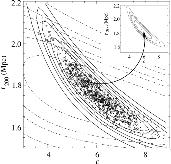
Figure 3: In this figure, the input lens model has an NFW profile with $\pi_{{\rm t}}$ of $c=6.0$ and r${}_{200}=1.75\leavevmode\nobreak\ {\rm Mpc}$, and the inner and outer radii of the annulus are $\theta_{\rm in}=0\hbox{$.\!\!^{\prime}$}6$, $\theta_{\rm out}=4\hbox{$.\!\!^{\prime}$}0$. The lens redshift is $z_{{\rm d}}=0.2$, and the other parameters are as described in the text. In the main panel, solid lines are contours of constant $\left\langle\ell_{\gamma}\right\rangle$ and dashed contours correspond to $\left\langle\ell_{\mu}\right\rangle$. Contours are drawn for $2\left\langle\Delta\ell\right\rangle=\{2.30,4.61,6.17,9.21,11.8,18.4\}$, within which one expects that 68.3%, 90%, 95.4%, 99%, 99.73% and 99.99% respectively, of parameter estimates from realisations will be enclosed. The crosses correspond to $\pi_{\rm max}$ recovered by applying the shear likelihood analysis to 1000 simulated data sets. The insert panel corresponds to a single, randomly chosen, realisation $\pi_{\rm max}$ with corresponding $\ell(\pi_{\rm max})$. Contours of constant $\ell_{\gamma}$ are drawn for $2({\ell}(\pi)-{\ell}(\pi_{\rm max}))=\{2.30,4.61,6.17,9.21\}$.

5.2 Can we distinguish between NFW and power-law profiles?

Two models commonly used to describe the radial dependence of the surface mass density are the NFW and power-law profiles, a specific case of which is the isothermal model. We briefly consider whether the shear method enables a distinction to be made between these profiles, and how much of a discrepancy there is between the best-fit models of each family.

The standard NFW lens was used to generate 500 catalogues of lensed galaxies, with $n_{\gamma}=30\leavevmode\nobreak\ {\rm arcmin}^{-2}$. Best-fit parameters were recovered in an aperture with inner radius $0\hbox{$.\!\!^{\prime}$}6$ and outer radius $4\hbox{$.\!\!^{\prime}$}0$, using the shear method and assuming (i) an NFW lens (parameters $c,r_{200}$), (ii) a lens with an isothermal slope, defined outside $\theta_{{\rm E}}$ [parameters $a$ (normalisation at $\theta_{{\rm E}}$) and $\theta_{{\rm E}}$] and (iii) a power-law lens (parameters $a$ and slope $q$), with $\theta_{{\rm E}}$ assumed to be known from observations, and set equal to that of the true NFW model. We refer to quantities associated with recovery under the true NFW model with the subscript “true”, and to those under other models with the subscript “false”.

Comparing $\ell_{\rm max,true}$ and $\ell_{\rm max,false}$ on a catalogue by catalogue basis shows that the NFW profile has a formally higher likelihood than the isothermal profile in 97.6% of cases. In practice, for a single data set, a particular profile would be considered to better describe the lens if it had a likelihood in excess of $\sim 2\sigma$ (depending on the observational noise) of other models considered. Evaluation of $2(\ell_{\rm max,true}-\ell_{\rm max,false})$ and comparison with the standard confidence-levels for normal distributions with 2 degrees of freedom shows that for 88.3 (71.7, 58.4, 39.6)% of the cases where the NFW profile is the most likely model, the ability to distinguish it from the isothermal profile is at greater than 68.3 (90, 95.4, 99)% confidence. In other words, for this case, distinguishing the NFW and isothermal models at 2$\sigma$ confidence is possible in about 60% of cases where the NFW model has a higher likelihood. These results are summarised in Table1. In cases where the isothermal fit is formally better, none of these realisations reach 68.3% confidence.

$\Upsilon$(%)	P$(>\Upsilon)$(%)
68.3	88.3
90.0	71.7
95.4	58.4
99.0	39.6

Table 1: The standard NFW lens was used to generate 500 catalogues of lensed galaxies, with $n_{\gamma}=30\leavevmode\nobreak\ {\rm arcmin}^{-2}$. Best-fit parameters were recovered in an aperture with $\theta_{\rm in}=0\hbox{$.\!\!^{\prime}$}6$ and $\theta_{\rm out}=4\hbox{$.\!\!^{\prime}$}0$. An NFW lens and an isothermal lens (parameterised as described in the text) were independently fit to the catalogues and their likelihoods compared. Considering cases where the NFW profile has a formally higher likelihood, and denoting the confidence level at which NFW and isothermal models can be distinguished by $\Upsilon$, the table shows P$(>\Upsilon)$ as a function of $\Upsilon$.

In the case of recovery with the more general power-law model, the best-fit NFW model has a higher likelihood in 67.8% of realisations, with 23.6% of these realisations being above the 68.3% confidence-level. For those realisations where the power-law model has a formally higher likelihood, a smaller fraction (10.6%) are above the 68.3% confidence-level, which is expected from the form of the distribution of $2(\ell_{\rm max,true}-\ell_{\rm max,false})$.

Just how different are the profiles corresponding to the best-fit parameters? To get an idea of how the statistics translate into observable differences, consider models obtained by taking the arithmetic mean of $\pi_{\rm max}$ at discrete distances from the lens centre, $\theta$ for the NFW parameters (the mean recovered values of $c$ and of $r_{200}$) and for the power-law models (the mean recovered values of $a$ and of $q$). The value of $|g(\@vec{\theta})_{\rm true}-g(\@vec{\theta})_{\rm false}|/|g(\@vec{\theta})_{\rm true}|$ is shown in Fig.5 as a function of $\theta$. At small radii the percentage difference is fairly large (but in this region it is observationally difficult to make measurements), dropping to zero at intermediate radii before increasing again to around 4%, dropping again to zero before slowly increasing at larger radii.

For illustration, $\theta_{\rm out}$ was increased to $15\hbox{$.\!\!^{\prime}$}0$ and 100 catalogues were generated using the NFW lens, and again the best-fit parameters were recovered using the two-parameter power-law model during the analysis. Comparison of the best-fit models shows that the NFW profile has a higher likelihood in 96% of cases; in 95 (82)% of these cases, the difference from the best power-law model is at greater than 68.3 (95.4)% confidence. When $\theta_{\rm out}$ is increased, note the marked increase in the percentage of cases where the true model has a higher likelihood, and at a higher confidence level.

In the future, space-based telecopes with a wide field-of-view will be available for studies of lensing clusters. To mimic the action of such a telescope, catalogue generation with the NFW profile and recovery with the NFW and power-law profiles was performed with $n_{\gamma}=150\leavevmode\nobreak\ {\rm arcmin}^{-2}$, with $\theta_{\rm out}=15\hbox{$.\!\!^{\prime}$}0$, giving $\approx\sqrt{5}$ increase in the signal-to-noise beyond that of the lower density case. With this extreme background density and data field size, all of the NFW best-fit models have higher likelihoods than the corresponding best-fit power-law models, at 99.99% significance difference. Another possible means to effectively increase $n_{\gamma}$ is by “stacking” large enough samples of ground based wide-field images of clusters. An analagous process has been undertaken for galaxy groups [see Hoekstra et al. 1999].

Figure 4: For 10000 simulated data sets, best-fit parameters were recovered using the shear method. The ratio of $P(>2\Delta\left\langle\ell_{\gamma}\right\rangle)$ to that expected if $2\Delta\left\langle\ell_{\gamma}\right\rangle$ followed a $\chi^{2}$ distribution is shown as a function of $2\Delta\left\langle\ell_{\gamma}\right\rangle$. On the top edge of the plot the 68.3%-, 90%-, 95.4%- and 99%-confidence intervals are marked.

Figure 5: The standard NFW lens was used to generate 500 catalogues of lensed galaxies. The best-fit parameters were recovered using the shear method in an aperture with $\theta_{\rm in}=0\hbox{$.\!\!^{\prime}$}6$, $\theta_{\rm out}=4\hbox{$.\!\!^{\prime}$}0$, and assuming (i) an NFW lens and (ii) a power-law lens. The figure shows $|g_{\rm true}-g_{\rm false}|/|g_{\rm true}|$ as a function of $\theta$, distance from the aperture centre. These values were obtained at discrete values of $\theta$ by taking the arithmetic mean of $g(\theta)$ for the 500 best-fit models.

5.3 Singular ellipsoidal profile

For this profile, the primary aim was to see how well the axial ratio and position angle of the SIE mass distribution could be recovered. The SIS is a special case of the SIE model ($f=1.0$), so we can also see how likely it is that an SIE will be misidentified as an SIS.

We considered the situation where the orientation of the SIE cluster is not well determined – i.e. where the free parameters are $f$ and the position angle $\alpha$. The values of $\pi_{\rm max}$ were recovered for 500 realisations, when $\alpha$ was set to 0.5 radians ($\approx 28.6^{\circ}$). A convenient representation of a cluster’s ellipticity is to write it in complex form as

$$\epsilon=\frac{1-f}{1+f}{\rm e}^{2{\rm i}\alpha}\equiv F{\rm e}^{2{\rm i}\alpha}.$$ (37)

Then the log-likelihood minimisation can be performed in the $\epsilon_{1}-\epsilon_{2}$ plane and in Fig.6 we mark the best-fit parameters $\pi_{\rm max}$ (${\epsilon}_{1}=F{\rm cos}(2\alpha)$ and ${\epsilon}_{2}=F{\rm sin}(2\alpha)$) with crosses (in this representation, $\pi_{{\rm t}}\equiv(0.06,0.0935)$). Note that $\alpha_{\rm max}=0.5\leavevmode\nobreak\ {\rm tan}^{-1}(\epsilon_{2}/\epsilon_{1})$ and that the distance from the origin is $F$.

The ensemble averaged log-likelihood function can be determined for the SIE by performing a 2-D numerical integration, either over the $f-\alpha$ plane or over the $\epsilon_{1}-\epsilon_{2}$ plane. Contours of constant $2\left\langle\ell_{\gamma}\right\rangle$ calculated in the $\epsilon_{1}-\epsilon_{2}$ plane are superimposed on Fig.6. Again, as in the case of circularly symmetric models, the spatial distribution of the realisations agrees well with the likelihood contours. The value of $f$ is well constrained - for instance, SIS models with $f=1.0$ lie outside the 95.4% confidence-level. As the value of $\alpha_{\rm true}$ is changed, then the locus of the centre of the ensemble averaged contours is a circle centred on the origin in the $\epsilon_{1}-\epsilon_{2}$ plane, and the areas of the confidence regions remain unchanged.

When $f_{{\rm t}}=1.0$ (i.e. the SIS case) $\alpha$ is unconstrained since the profile is circular; as $f_{{\rm t}}$ is decreased, the ability to constrain $\alpha$ increases.

Figure 6: An SIE lens at $z_{{\rm d}}=0.2$ with $\theta_{\rm E}=0\hbox{$.\!\!^{\prime}$}5$ and $\pi_{{\rm t}}$: $f=0.8$, $\alpha=0.5\leavevmode\nobreak\ {\rm radians}$ was used to generate 500 catalogues of lensed galaxies. The best-fit parameters were recovered using the shear method in an aperture with $\theta_{\rm in}=1\hbox{$.\!\!^{\prime}$}0,\theta_{\rm out}=3\hbox{$.\!\!^{\prime}$}0$. The panel shows $\epsilon_{1}$ and $\epsilon_{2}$ (the components of the complex ellipticity of the cluster) for the $\pi_{\rm max}$ (crosses). Contours of constant $\left\langle\ell_{\gamma}\right\rangle$ for $2\Delta\ell=\{2.3,4.61,6.17,9.21,11.8,18.4\}$ are indicated by the solid lines.

6 Redshift distribution

Throughout this Section, the catalogue generation and best-fit model recovery were performed using a cluster described by an NFW profile, $\pi_{\rm t}$: $c=4.0$, $r_{200}=1.0\leavevmode\nobreak\ {\rm Mpc}$, at $z_{{\rm d}}=0.5$. The number density of sources was taken to be $n_{\gamma}=40\leavevmode\nobreak\ {\rm arcmin}^{-2}$. Five hundred catalogues of lensed galaxies were generated in an aperture with $\theta_{\rm in}=0\hbox{$.\!\!^{\prime}$}2$ and $\theta_{\rm out}=6\hbox{$.\!\!^{\prime}$}0$, following the prescription given in Section 4. The best-fit parameters were recovered independently under each redshift knowledge scenario outlined in Section 3.2.

When photometric redshifts ($z_{\rm ph}$) were assumed to be available, these were assigned by adding a Gaussian random deviate of dispersion $\sigma_{z}=0.1$ to the true redshift $z_{t}$. During the analysis, the photometric estimates were inserted in place of the true redshifts. As mentioned previously, their dispersion can be thought of as a modification of $\sigma_{{\epsilon}}$, giving an effective dispersion $\sigma_{\rm eff}$. From our analytic estimate, we would expect that the error on parameters recovered would not differ much from the ideal case. This has also been indicated by Bartelmann & Schneider (2000).

In the case where the galaxies were placed on a sheet, the value of $\left\langle w\right\rangle$ was determined for the lens at $z_{{\rm d}}=0.5$. For $p(z){{\rm d}}z$ in question, $\left\langle w\right\rangle=0.35$, which corresponds to $z_{\rm sheet}=0.82$. The values $\left\langle w\right\rangle^{2}=0.125$ and $\left\langle w^{2}\right\rangle=0.185$ imply that $\left\langle g_{t}\right\rangle/\left\langle g_{\rm sheet}\right\rangle\approx 1+0.48\kappa$; this means that the cluster mass is overestimated with the sheet approximation, since it must be more massive to produce the same lensing signal. For typical values of $\kappa\sim 0.1$, the correction is fairly small.

When the form of the redshift distribution is known, but not the redshifts of individual galaxies, Eq.(19) was discretised and integrated numerically.

Fig.7 shows the recovered $\pi_{\rm max}$ for the ideal case when all redshifts are known (squares) and for the case where the sources are at $z_{\rm sheet}$ (crosses), to give an indication of the scatter. Error matrices were obtained from the values of $\pi_{\rm max}$ for each case. Denoting $(c-c_{{\rm t}})$ by ${\cal G}_{1}$ and $(r_{200}-r_{200_{\rm t}})$ by ${\cal G}_{2}$, then the elements are ${\cal G}_{ij}\equiv\left\langle{\cal G}_{i}{\cal G}_{j}\right\rangle$. Then, error ellipses were obtained from the eigenvalues and eigenvectors of these matrices. The inner ellipse corresponds to the true redshift case, and the outer ellipse to the sheet case.

The relative error matrices were derived from the values of $\pi_{\rm max}$ for each of the redshift assumptions. Denoting $(c-c_{{\rm t}})/c_{{\rm t}}$ by ${\cal E}_{1}$ and $(r_{200}-r_{200_{\rm t}})/r_{200_{\rm t}}$ by ${\cal E}_{2}$, then the elements are ${\cal E}_{ij}\equiv\left\langle{\cal E}_{i}{\cal E}_{j}\right\rangle$. The elements of the relative error matrices are shown in Table2.

Naturally, when all the source redshifts are known, the dispersion of $\pi_{\rm max}$ is smallest. If photometric redshifts are available, then the dispersion is only marginally greater $(\sim 1.5\%)$, which we expected from our estimate. The dispersion becomes greater when only the distribution is known $(\sim 21\%)$, or greater still when the sources are assumed to be on a sheet $(\sim 60\%)$. The advantage of having redshift information becomes more paramount as the redshift of the lens is increased – recall from before that if a cluster is at a low redshift, then the redshift distribution is fairly unimportant. Also, if $\kappa$ is large this information is also more important since the errors incurred by making a sheet approximation become large.

Redshift Scenario	${\cal E}_{11}$	${\cal E}_{12}$(Mpc)	${\cal E}_{22}$(Mpc2)
True redshifts	0.063	-0.0101	0.00345
Photometric redshifts	0.063	-0.0103	0.00358
Redshift distribution	0.069	-0.014	0.007
Sheet	0.11	-0.014	0.005

Table 2: An NFW cluster at $z_{{\rm d}}=0.5$ and with $\pi_{t}$: $c=4.0$, $r_{200}=1.0\leavevmode\nobreak\ {\rm Mpc}$ was used to generate 500 catalogues of lensed galaxies. Best-fit parameters were recovered under different assumptions of redshift knowledge, indicated in the left-hand column. The elements of the relative error matrices (see text for details) are given in the right-hand columns.

Figure 7: An NFW lens at $z_{{\rm d}}=0.5$, $\pi_{t}$: $c=4.0$, $r_{200}=1.0\leavevmode\nobreak\ {\rm Mpc}$, was used to generate 500 catalogues of lensed galaxies, where $p(z){\rm d}z$ for the source galaxies is as described in the text. Best-fit parameters were recovered using the shear method in an aperture with $\theta_{in}=0\hbox{$.\!\!^{\prime}$}2$, $\theta_{\rm out}=6\hbox{$.\!\!^{\prime}$}0$. The squares show parameters recovered when the true redshifts are known individually and the crosses show recovery when the source galaxies are placed at $z_{\rm sheet}$. The 68.3% confidence ellipses were determined from the eigenvectors and eigenvalues of the error matrices, and are shown for the true redshift (inner ellipse) and sheet case (outer ellipse).

We can compare these results with the analytic work presented in Bartelmann & Schneider (2000) who focused on the dispersion of shear estimates in the cases where all redshifts are known, and where only the distribution $p(z){{\rm d}}z$ is known. Although many of their input parameters are different, a qualitative comparison can be made. For instance, at $z_{{\rm d}}=0.5$ they find an improvement of $30\%$ in the accuracy of the shear estimate when redshifts are known, as opposed to when only $p(z){{\rm d}}z$ is known - we obtain a similar result: $\sim 21\%$ improvement in the dispersion of recovered $\pi_{\rm max}$ between these two cases.

7 The influence of substructure

In the preceeding sections we considered smooth parametric models of clusters, for analytical and numerical simplicity. The full treatment of substructure requires studying how its spatial distribution and power spectrum interplay with the smooth cluster profile and the aperture within which the observations are made. This is beyond the scope of this work and will be investigated in a forthcoming paper. Here we illustrate the implications of substructure on the analysis, by constructing a non-smooth toy model consisting of a smooth NFW cluster ($z_{{\rm d}}=0.2$, $c=6.0$ and $r_{200}=1.75\leavevmode\nobreak\ {\rm Mpc}$), with surface mass density $\kappa_{\rm smooth}(r)$, which is modified by the addition of smaller scale sub-profiles, denoted by $\kappa_{\rm sub}(r)$. In order to preserve the overall mass of the cluster, $\kappa_{\rm sub}(r)$ has to be chosen so that $2\pi\int_{0}^{r_{\rm sub}}r\kappa_{\rm sub}(r){{\rm d}}r=0$, where $\kappa_{\rm sub}$ is defined for $r<r_{\rm sub}$. A suitable functional form is

$$\kappa_{\rm sub}(r) = \kappa_{\rm sub_{c}}\frac{16}{\pi}\left(0.25-\left(\frac{r}{r_{\rm sub}}\right)^{2}\right)$$ (38)

$$\times \left(1-\left(\frac{r}{r_{\rm sub}}\right)^{2}\right)^{2},$$

where $(4/\pi)\kappa_{\rm sub_{c}}$ is the central surface mass density. Below, we take $r_{\rm sub}=1\hbox{$.\!\!^{\prime}$}0$ and amplitude scales $\kappa_{\rm sub_{c}}=0.01,0.025$ and 0.05. The magnitude of the corresponding shear field is

$$|\gamma_{\rm sub}|(r) = \kappa_{\rm sub_{c}}\frac{4}{\pi}\biggl{(}3\left(\frac{r}{r_{\rm sub}}\right)^{2}-6\left(\frac{r}{r_{\rm sub}}\right)^{4}$$ (39)

$$+ 3\left(\frac{r}{r_{\rm sub}}\right)^{6}\biggr{)},$$

and the phase is determined from the position angle relative to the centre of the sub-profile. The final surface mass density is simply a linear superposition of the smooth and $n$ sub-profiles,

$$\kappa_{\rm tot}(r)=\kappa_{\rm smooth}(r)+\sum_{n}\kappa_{\rm sub}(r),$$ (40)

and similarly for the shear field $\gamma$,

$$\gamma_{\rm tot}(r)=\gamma_{\rm smooth}(r)+\sum_{n}\gamma_{\rm sub}(r).$$ (41)

Finally, the reduced shear is

$$g_{\rm tot}(r)=\frac{\gamma_{\rm tot}(r)}{1-\kappa_{\rm tot}}.$$ (42)

Catalogues of lensed galaxies were generated using the prescription above, with 500 equal amplitude sub-profiles distributed between $0\hbox{$.\!\!^{\prime}$}0$ and $15\hbox{$.\!\!^{\prime}$}0$ from the cluster centre, their number density decreasing with radius. The resulting $\kappa_{\rm tot}$ inside a $4\hbox{$.\!\!^{\prime}$}0$ radius is shown in Fig.8, for $\kappa_{\rm sub_{c}}=0.05$. The shear likelihood analysis was performed to obtain the best-fit smooth model consistent with the data.

Figure 8: This figure shows $\kappa_{\rm tot}$ over an 8$.\!\!^{\prime}$0 field, resulting when 500 sub-profiles of amplitude $\kappa_{\rm sub_{c}}=0.05$ (see text for further details) are added to an NFW cluster ($z_{{\rm d}}=0.2$, $c=6.0$ and $r_{200}=1.75\leavevmode\nobreak\ {\rm Mpc}$). The contours shown correspond to $\kappa_{\rm tot}=0.025,0.05,0.1,0.15,0.2,0.3,0.4,0.5$.

With substructure the advantages of using data close to the centre of the lens, are counteracted by the disadvantage of the increased deviation from the smooth value of $g_{\rm tangential}(r)$. Here we restrict our consideration to one of our standard apertures with $\theta_{\rm in}=0\hbox{$.\!\!^{\prime}$}6$ and $\theta_{\rm out}=4\hbox{$.\!\!^{\prime}$}0$.

First of all, in generating each lensed catalogue we allowed both the spatial distribution of the substructure, and the spatial and ellipticity distribution of the background galaxies to vary. In the second instance, the distribution of background galaxies was kept fixed, so that the contribution of randomising the substructure to the results could be disentangled. We recovered $\pi_{\rm max}$ for the smooth input profile, and for input profiles with $\kappa_{\rm sub_{c}}=0.01,0.025$ and 0.05.

The relative error matrices were derived from the values of $\pi_{\rm max}$ for each of the smooth and substructure cases. Denoting $(c-c_{{\rm t}})/c_{\rm t}$ by ${\cal E}_{1}$ and $(r_{200}-r_{200_{\rm t}})/r_{200_{\rm t}}$ by ${\cal E}_{2}$, then the elements of the matrices are ${\cal E}_{ij}\equiv\left\langle{\cal E}_{i}{\cal E}_{j}\right\rangle$; these are given in Table3. One can also compare the log-likelihoods of the $\pi_{\rm max}$ for each of the catalogues generated with substructure, and the catalogue generated from the smooth profile (both analysed assuming a smooth profile, as mentioned above). Fig.9 shows histograms of $2\Delta\ell$ for $\kappa_{\rm sub_{c}}=0.01$ (solid line), 0.025 (short dashed line) and 0.05 (long dashed line). In the case where the amplitude $\kappa_{\rm sub_{c}}=0.01$, the associated error matrix is statistically indistinguishable from that of the smooth profile. As the amplitude increases, the error on the recovered parameters increases as does $2\Delta\ell$.

Substructure Scenario	${\cal E}_{11}$	${\cal E}_{12}$(Mpc)	${\cal E}_{22}$(Mpc2)
A	0.018	-0.0069	0.0030
B	0.021	-0.0070	0.0028
C	0.033	-0.0089	0.0029
D	0.083	-0.0173	0.0042
E	0.055	-0.0083	0.0018

Table 3: An NFW cluster at $z_{{\rm d}}=0.2$, $\pi_{t}$: $c=6.0$, $r_{200}=1.75\leavevmode\nobreak\ {\rm Mpc}$ and with various degrees of substructure was used to generate 100 catalogues of lensed galaxies. The scenarios indicated in the left-hand column are as follows: A correponds to the smooth profile, and the random factor of each of the realisations is the spatial distribution and intrinsic ellipticities of the background galaxies. For scenarios B, C and D, 500 sub-profiles with $\kappa_{\rm sub_{c}}=0.01,0.025$ and 0.05 respectively were added to the smooth profile and for each realisation the background galaxies and the spatial distribution of the substructure were random. Finally, for E the background galaxy distribution was kept fixed and only the spatial distribution of the substructure was randomised, with $\kappa_{\rm sub_{c}}=0.05$. The elements of the relative error matrices (see text for details) are given in the right-hand columns.

Figure 9: Various amplitudes of sub-profiles were added to an NFW cluster at $z_{{\rm d}}=0.2$, $\pi_{t}$: $c=6.0$, $r_{200}=1.75\leavevmode\nobreak\ {\rm Mpc}$, which was then used to generate 100 catalogues of lensed galaxies and the best-fit smooth model was recovered. This figure shows the distribution of $2\Delta\ell$, calculated for $\kappa_{\rm sub_{c}}=0.01$ (solid line), 0.025 (short dashed line) and 0.05 (long dashed line).

8 Discussion and conclusions

Fitting parameterised models to clusters is essential when a statistical comparison is to be made between them. This is becoming especially important with the explosion in the use of wide field imagers to study cluster samples. The aims are to ascertain the best method to constrain these models, and to be able to predict the uncertainties in parameters obtained given observations of different depths, data field size and level of knowledge of the redshift distribution of the galaxy population. We find that likelihood and ensemble averaged likelihood techniques are an excellent means to achieve these goals.

In this paper we compared the accuracy with which parameters can be fit to lower redshift clusters described by NFW profiles (parameters $c$ and $r_{200}$), using the shear and magnification information. We find that
(i) for the case considered, the shear method is superior, although there is a marked degeneracy in the determination of the concentration parameter, $c$.
(ii) The analytic treatment is consistent with the results of Monte Carlo simulations, and that the assumption of $\chi^{2}$-statistics is a good approximation.

To investigate whether we can distinguish between NFW and power-law models, catalogues of lensed galaxies were generated using an NFW model, and parameters recovered under an NFW and power-law model independently:
(iii) The ability to distinguish between profiles depends strongly on the size of the field-of-view used in the lensing analysis, and on the number density of sources. For example, for the model considered, when $\theta_{\rm out}$ is increased from $4\hbox{$.\!\!^{\prime}$}0$ to $15\hbox{$.\!\!^{\prime}$}0$ there is a $\sim 40\%$ improvement in the ability to distinguish between 2 parameter NFW and power-law models.

In practice, other factors that would have to be taken into account include how close to the centre of the cluster it is possible to take useful data, and other sources of noise in the observations. The number density of galaxies available for the analysis will depend on the limiting magnitude of the observations, and the seeing conditions. As to the issue of the PSF anisotropy, which hampers the accurate measurement of galaxy shapes, detailed simulations using realistic PSF profiles have been undertaken by Erben et al. (2000); these show that gravitational shear can be recovered with an error of 10-15%. Similar work is presented by Bacon et al. (2000). Gray et al. (2000) recently applied the maximum likelihood magnification method to infrared CIRSI observations of Abell 2219, fitting single parameter SIS ($\theta_{{\rm E}}$) and NFW ($r_{{\rm s}}$) profiles. However, with the noise in their observations it was not possible to differentiate between the profiles.

The position angle of the luminous and dark matter distributions may be significantly misaligned. By considering the SIE profile, we have shown
(iv) at what confidence the complex ellipticity of a cluster can be recovered,
(v) In the case of this non-circulary symmetric profile, we have also demonstrated that our numerical simulations are consistent with the ensemble averaged log-likelihood confidence-intervals.

We also examined the dispersion in recovered parameters for an NFW cluster at a higher redshift ($z_{\rm d}=0.5$), assuming several possibilities for our knowledge of the redshift distribution of source galaxies. Since we are moving into an era when photometric redshifts with $\sigma_{z}\approx 0.1$ are becoming available for large samples of galaxies, a striking conclusion is that
(vi) the fractional gain in the accuracy of parameter estimates is only $\sim 1.5\%$ more when exact redshifts are known rather than photometric estimates.
(vii) If only $p(z){\rm d}z$ is known, then the fractional gain in having spectroscopic redshifts is $\sim 21\%$.
(viii) The most common assumption in weak lensing analyses for the source redshift distribution - that they lie on a sheet whose redshift is determined by $\left\langle w\right\rangle$ - gives parameters with the largest errors, and having spectroscopic or photometric redshifts would decrease their dispersion by $\sim 60\%$. If colour or redshift information is available which enables some fraction of foreground or cluster galaxies to be identified and excluded from the analysis, then the dispersion in parameter estimates becomes lower.

Throughout for simplicity we assumed an EdS cosmology; qualitatively, our conclusions are unaffected by this and quantitatively the discrepancy is small. The cosmological weighting function $w(z)$ is readily evaluated for any cosmological model, and the difference in an $\Omega_{0}=0.3,\Omega_{\Lambda}=0.7$ cosmology is less than 10% even when the lens redshift $z_{{\rm d}}=0.8$ [see Bartelmann & Schneider (2000)]. In any case, changing the cosmological model is equivalent to applying a small change to the anyway uncertain redshift distribution.

Finally, we qualitatively considered how fitting parameterised models to lensing data is influenced by the presence of substructure. Our preliminary work will be developed in a forthcoming paper. In the framework of our basic model, we find that
(ix)increasing the amplitude of the substructure increases the dispersion of the recovered parameters.

- (1) Alcock C. 2000, Science 287, 73
- (2) Bacon D., Refregier A., Clowe D., Ellis R. astro-ph/0007023, submitted to MNRAS
- (3) Bartelmann M., Schneider P. astro-ph/9912508, Physics Reports, in press
- (4) Benítez N. 2000, ApJ 536, 571
- (5) Brainerd T.G., Blandford R.D., Smail I. 1996, ApJ 466, 623
- (6) Broadhurst T.J., Taylor A.N., Peacock J.A. 1995, ApJ 438, 49
- (7) Canizares C.R. 1982, ApJ 263, 508
- (8) Clowe D., Luppino G.A., Kaiser N., Henry J.P., Gioia I. 1998, ApJ 497, L61
- (9) Clowe D., Luppino G.A., Kaiser N., Gioia I.M. 2000, ApJ 539, 540
- (10) Connolly A.J., Csabai I., Szalay A.S., Koo D.C., Kron R.G., Munn J.A. 1995, AJ 110, 2655
- (11) Dye S., Taylor A.N., Thommes E.M., Meisenheimer K., Wolf C., Peacock J.A. astro-ph/0002011, submitted to MNRAS
- (12) Erben T., Van Waerbeke L., Bertin E., Mellier Y., Schneider P. astro-ph/0007021, A&A, in press
- (13) Fernández-Soto A., Lanzetta K.M., Yahil A. 1999, ApJ 513, 34
- (14) Fischer P., Tyson A.J. 1997, AJ 114, 14
- (15) Fort B., Mellier Y., Dantel-Fort M. 1997, A&A 321, 353
- (16) Geiger B., Schneider P. 1998, MNRAS 295, 497
- (17) Geiger B., Schneider P. 1999, MNRAS 302, 118
- (18) Gray M.E., Ellis R.S., Refregier A., Bezecourt J., McMahon R.G.,Beckett M.G, MacKay C.D., Hoenig M.D. 2000, MNRAS 318, 573
- (19) Hoekstra H., Franx M., Kuijken K., Squires G. 1998, ApJ 504, 636
- (20) Hoekstra H., Franx M., Kuijken K. 1999, astro-ph/9911106
- (21) Hoekstra H., Franx M., Kuijken K. 2000, ApJ 532, 88
- (22) Jing Y.P. 2000, ApJ 535, 30
- (23) Kaiser N., Squires G. 1993, ApJ 404, 441
- (24) Keeton C.R., Kochanek C.S. Falco E.E. 1998, ApJ 509, 561
- (25) Moore B., Gelato S., Jenkins A., Pearce F.R., Quilis V. 2000, ApJ 535L, 21
- (26) Navarro J.F., Frenk C.S., White S.D.M. 1996, ApJ 462, 563
- (27) Navarro J.F., Frenk C.S., White S.D.M. 1997, ApJ 490, 493
- (28) Press W.H., Teukolsky S.A., Vetterling W.T., Flannery B.P. 1992, in Numerical recipes in FORTRAN. The art of scientific computing, Cambridge: University Press, 2nd Edn.
- (29) Schneider P., Seitz C. 1995, A&A 294, 411
- (30) Schneider P., Ehlers J., Falco E.E. 1992, Gravitational lenses, Springer: New York (SEF)
- (31) Schneider P., King L.J., Erben T. 2000, A&A 353, 41
- (32) Schramm T., Kayser R. 1995, A&A 289 L5
- (33) Seitz C., Schneider P. 1997, A&A 318, 687
- (34) Van Waerbeke L. et al. 2000, A&A 358, 30
- (35) Wright C.O., Brainerd T.G. 2000, ApJ 534, 34