Source-lens clustering effects on the skewness of the lensing convergence

Abstract

The correlation between source galaxies and lensing potentials causes a systematic effect on measurements of cosmic shear statistics, known as the source-lens clustering (SLC) effect. The SLC effect on the skewness of lensing convergence, $S_{3}$, is examined using a nonlinear semi-analytic approach and is checked against numerical simulations. The semi-analytic calculations have been performed in a wide variety of generic models for the redshift distribution of source galaxies and power-law models for the bias parameter between the galaxy and dark matter distributions. The semi-analytic predictions are tested successfully against numerical simulations. We find the relative amplitude of the SLC effect on $S_{3}$ to be of the order of five to forty per cent. It depends significantly on the redshift distribution of sources and on the way the bias parameter evolves. We discuss possible measurement strategies to minimize the SLC effects.

1 Introduction

Recent detections of the cosmic shear signal have opened a new window to probe the distribution of matter in the Universe, its evolution, and to test cosmological models (Van Waerbeke et al. 2000; Wittman et al. 2000; Bacon, Refregier & Ellis 2000; Kaiser, Wilson & Luppino 2000; Maoli et al 2001). These detections have been obtained from relatively small fields so far, which limits the statistical analysis of the surveys to second order moments, the variance or two-point correlation function of cosmic shear. The amplitude of second order statistics reflects that of density fluctuations and roughly scales as $\sigma_{\gamma}\propto\Omega_{\rm m}^{0.6-0.8}\sigma_{8}$ at large scale (Bernardeau, Van Waerbeke & Mellier 1997, hereafter BvWM97) and $\sigma_{\gamma}\propto\Omega_{\rm m}^{0.6-0.8}\sigma_{8}^{1.2-1.3}$ at small scale (Jain & Seljak 1997; Maoli et al. 2001). On the other hand, the skewness (a third order statistic) of lensing convergence is known to be sensitive to $\Omega_{\rm m}$, almost independently of $\sigma_{8}$ (BvWM97). Therefore, combined analysis of the skewness and the variance will provide precious constraints on both values of $\Omega_{\rm m}$ and $\sigma_{8}$. As a consequence, skewness detection and measurement is one of main goals of on-going wide field cosmic shear surveys such as the DESCART project.

Cosmic shear statistics have been studied analytically (see Mellier 1999 and Bartelmann & Schneider 2001 for reviews and references therein) as well as numerically (Jain, Seljak & White 2000; White & Hu 2000). The skewness of lensing convergence was first calculated by BvWM97 based on a quasi-linear perturbation theory approach. It has been, however, recognized that this approach is not robust enough to provide accurate predictions for the value of the skewness over the whole available dynamic range. In particular, the two following points have to be addressed and carefully included in the calculations: (i) Nonlinear growth of the density field: numerical studies show that nonlinear growth enhances skewness especially at angular scales smaller than one degree (Jain et al. 2000; White & Hu 2000; Van Waerbeke et al. 2001b). (ii) Source clustering: Bernardeau (1998) (hereafter B98) pointed out that correlations between source galaxies and lensing potential reduce skewness amplitude. B98 underlined that this effect is sensitive to the redshift distribution of sources.

The purpose of this paper is to examine the effect of source clustering (SLC) on measurements of the skewness of lensing convergence. Special attention is payed to its dependence on the redshift distribution of sources and on evolution of the bias relation between matter and galaxy distribution. Since the redshift distribution of faint galaxies is uncertain and little is known about the bias, this paper does not aim at making accurate predictions for the amplitude of SLC effect in real cosmic shear surveys. Our objective is to estimate its magnitude in order to propose strategies that minimize its effects.

We basically follow the perturbation theory approach first developed by B98 but generalize it in two ways: (i) we take into account the effects of nonlinear evolution of the density field, adopting the nonlinear semi-analytic ansatz developed by Jain & Seljak (1997) and Van Waerbeke et al. (2001b); (ii) we allow a possible redshift dependence of the bias parameter, $b(z)=b_{0}(1+z)^{\gamma}$ and examine the cases $\gamma=0$ to 2. Moreover we consider three cosmological Cold Dark Matter family models (CDM), two flat models with and without cosmological constant and an open model, and 12 different models for the source distribution which cover a wide range of mean redshift and width for the distribution.

Finally, for the first time the accuracy of semi-analytic predictions for the SLC effects on the skewness is tested against numerical simulations in standard CDM model.

The outline of this paper is as follows. In section 2, the physical mechanism of SLC is described. In section 3, an expression for the skewness of lensing convergence is presented that takes both SLC and nonlinear evolution of the density field into account. In section 4, our models are described. Results of the semi-analytic approach are presented in section 5. In section 6, semi-analytic predictions are tested against numerical simulations. We summarize and discuss our conclusions in section 7. The derivation of the convergence skewness in the presence of the SLC is presented in Appendix A. The $N$-body data sets and the ray-tracing method used for this work are described in Appendix B. In Appendix C, details of the procedure to generate mock galaxy catalogues are presented.

2 What is the SLC effect?

Figure 1: An illustration of the correlation between the gravitational potential (contour lines) and the population of sources (denoted by filled circles).

The SLC effect discussed in this paper comes to light because of the conjunction of three circumstances, namely: (i) source galaxies are not randomly distributed in the sky but are correlated; (ii) the source galaxy distribution traces somehow the matter field; (iii) the redshift distribution of source galaxies is rather broad. The width of the distribution depends on source selection criterion, and generally, the distribution of source galaxies overlaps with the distribution of lensing structures, so source galaxies are somehow correlated with the lensing potential. This correlation causes systematic effects on measurements of cosmic shear, that may be illustrated as follows. Figure 1 shows a distribution of sources (denoted by filled circles) and the gravitational potential (contour lines). For line-of-sight 1 (LOS 1), the distant galaxies are lensed by the gravitational potential located at an intermediate distance and thus have a high positive lensing convergence. This high signal is reduced by the excess of foreground sources bound to the foreground gravitational potential which, in contrast, has a low lensing. On the other hand, for a line-of-sight 2 (LOS 2), distant sources are lensed by the foreground void and thus have a negative lensing convergence. This negative signal is amplified because of the lack of foreground sources in the void. Accordingly, the probability distribution function of the lensing convergence, which is skewed toward a high value in absence of the SLC (e.g., BvWM97, Jain et al. 2000) becomes more symmetric than for the case of a random distribution of source galaxies. As a result, the amplitude of skewness of lensing convergence drops.

As was pointed out by B98, there is another possible effect caused by intrinsic clustering of source galaxies. The average distance of sources and their sky density may indeed vary from one direction to another, which can cause additional systematic effects on the cosmic shear statistics (these effects was included in the definition of source clustering used by B98). It was pointed out by B98 and Thion et al. (2001) that this effect on the convergence skewness is in general very small. Therefore, in this analysis, we do not take it into account for the analytical calculations presented in next section, although it will be obviously present in the numerical experiments discussed in § 6.

3 The perturbation theory approach

3.1 The quasi-linear regime

The expressions for the skewness of lensing convergence and the correlation term due to SLC were first derived by BvWM97 and B98 in the framework of perturbation theory. In this subsection, we only summarize expressions which are directly relevant to this paper. Detailed derivations and notations are given in Appendix A.

In the presence of the SLC, the skewness parameter, defined by $S_{3}(\theta)=\langle\kappa_{\theta}^{3}\rangle/V_{\kappa}^{2}(\theta)$, consists of two terms; namely, one arises from the quasi-linear theory and the other from SLC:

$$S_{3}(\theta)=S_{3}^{\rm q.l.}(\theta)+S_{3}^{\rm slc}(\theta),$$ (1)

with

$$S_{3}^{\rm q.l.}(\theta) = {{\langle\kappa_{\theta}^{3}\rangle^{q.l.}}\over{V_{\kappa}^{2}(\theta)}}$$ (2)

$$= {6\over{V_{\kappa}^{2}(\theta)}}\left({{H_{0}}\over c}\right)^{3}\int_{0}^{\chi_{H}}d\chi\,w^{3}(\chi)$$

$$\times\left[{6\over 7}I_{0}^{2}(\chi,\theta)+{1\over 4}I_{0}(\chi,\theta)I_{1}(\chi,\theta)\right],$$

$$S_{3}^{\rm slc}(\theta) = {{\langle\kappa_{\theta}^{3}\rangle^{\rm slc}}\over{V_{\kappa}^{2}(\theta)}}$$

$$= {{9\Omega_{\rm m}}\over{V_{\kappa}^{2}(\theta)}}\left({{H_{0}}\over c}\right)^{3}\int_{0}^{\chi_{H}}d\chi\,n_{s}(\chi)b(\chi)w(\chi)I_{0}(\chi)$$

$$\times\int_{0}^{\chi}d\chi^{\prime}\,g(\chi^{\prime},\chi)w(\chi^{\prime})I_{0}(\chi^{\prime})$$

$$-{6\over{V_{\kappa}(\theta)}}{{H_{0}}\over c}\int_{0}^{\chi_{H}}d\chi\,n_{s}(\chi)b(\chi)w(\chi)I_{0}(\chi).$$

In these equations,

• $\theta$ is the size of the smoothing window,

• $H_{0}/c$ is the Hubble constant in speed of light units,

• $V_{k}(\theta)$ is the variance of the lensing convergence [given by eq. (22)],

• $\chi$ denotes the radial comoving distance (and $\chi_{H}$ corresponds to the horizon),

• $w(\chi)$ is the lensing efficiency function [eq. (18)],

• functions $I_{0}(\chi,\theta)$ and $I_{1}(\chi,\theta)$ depend on the power-spectrum of matter density fluctuations through eqs. (23) and (26),

• $\Omega_{\rm m}$ is the matter density in units of the critical density,

• $n_{s}[\chi(z)]$ the average number density of sources,

• function $g(\chi_{l},\chi_{s})$ is given by eq. (15),

• $b(\chi)$ is the linear biasing function between the galaxy and the matter density contrast.

3.2 Nonlinear regime

For the variance of the lensing convergence, the effect of nonlinear evolution of the density power spectrum can be included by replacing the linear power spectrum (which enters the above expressions through $V_{\kappa}(\theta)$, $I_{0}(\chi)$ and $I_{1}(\chi)$, see Appendix A for their explicit expressions) with the nonlinear power spectrum, i.e., $P_{\rm lin}(a,k)\rightarrow P_{\rm NL}(a,k)$ (Jain & Seljak 1997). We use the fitting formula of nonlinear power spectrum given by Peacock and Dodds (1996). This semi-analytic approach has been tested against ray-tracing simulations, and a good agreement between the numerical results and the semi-analytic predictions was found (Jain et al 2000; White and Hu 2000).

In the framework of perturbation theory, all density contrasts needed for the calculation of the skewness correction term [equation (3.1)] correspond to linear order (see B98 for details). This comes from the fact that the quantity to be computed, an angular average of projected fourth moments, is given by the product of two two-point correlations: its intrinsic connected part has a negligible contribution because of the projection effects. The incorporation of the nonlinear effects is then straightforward. As for the variance, it amounts to formally replacing the linear power spectrum with the nonlinear one.

The semi-analytic calculation of the skewness in the nonlinear regime was developed by Van Waerbeke et al. (2001b). It is based on the fitting formula of the density bispectrum by Scoccimarro & Couchman (2000) and is given by

$$S_{3}^{\rm n.l.}(\theta) = {1\over{V_{\kappa}^{2}(\theta)}}{6\over{(2\pi)^{4}}}\left({{H_{0}}\over c}\right)^{3}\int_{0}^{\chi_{\rm max}}d\chi\,w^{3}(\chi)$$ (4)

$$\times\int d^{2}{\bf k_{1}}\,P_{\rm NL}(k_{1})W[k_{1}f(\chi)\theta]$$

$$\times\int d^{2}{\bf k_{2}}\,P_{\rm NL}(k_{2})W[k_{2}f(\chi)\theta]$$

$$\times W[|{\bf k_{1}}+{\bf k_{2}}|f(\chi)\theta]F_{2}^{\rm eff}({\bf k_{1}},{\bf k_{2}}),$$

with

$$F_{2}^{\rm eff}({\bf k_{1}},{\bf k_{2}}) = {5\over 7}a(n,k_{1})a(n,k_{2})$$ (5)

$$+{1\over 2}b(n,k_{1})b(n,k_{2}){{{\bf k_{1}}\cdot{\bf k_{2}}}\over{k_{1}k_{2}}}\left({{k_{1}}\over{k_{2}}}+{{k_{2}}\over{k_{1}}}\right)$$

$$+{2\over 7}c(n,k_{1})c(n,k_{2}){({{\bf k_{1}}\cdot{\bf k_{2}}})^{2}\over{|k_{1}|^{2}|k_{2}|^{2}}}.$$

Here, the notations are as follows:

• $k=|{\bf k}|$,

• $f(\chi)$ denotes the comoving angular diameter distance (see Appendix A),

• $W$ is the Fourier transform of the smoothing window,

• functions $a(n,k)$, $b(n,k)$ and $c(n,k)$ depend on the effective power spectral index $n$ at scale $k$ (explicit expressions are given in Scoccimarro & Couchman 2000; see also Van Waerbeke et al. 2001b).

It should be noted that, since the bispectrum fitting formula is constructed via the dark matter bispectrum measured from only one $N$-body simulation data set, there is about a 10-20 per cent uncertainty in the fitting formula. This is mainly a cosmic variance effect (Van Waerbeke et al. 2001b).

4 Models

4.1 Cold dark matter models (CDM)

Table 1: Cosmological parameters for the models considered in this paper. $\Omega_{\rm m}$ is the matter density in units of the critical density and similarly for the cosmological constant $\Omega_{\lambda}$; $h\equiv H_{0}/100$ is the Hubble constant in units of $100$ km s^-1 Mpc^-1; $\sigma_{8}$ is the variance of the dark matter distribution in a sphere of radius $8\,h^{-1}$ Mpc.

Model	$\Omega_{\rm m}$	$\Omega_{\lambda}$	$h$	$\sigma_{8}$
SCDM	1.0	0.0	0.5	0.6
OCDM	0.3	0.0	0.7	0.85
$\Lambda$CDM	0.3	0.7	0.7	0.9

We discuss three Cold Dark Matter (CDM) models, a flat model with ($\Lambda$CDM) and without cosmological constant (SCDM) and an open model (OCDM), using galaxy cluster abundances to normalize the power-spectrum (Eke, Cole & Frenk, 1996; Kitayama & Suto 1997) and the formula of Bond & Efstathiou (1984) for the transfer function. The parameters of the models are listed in Table 1.

4.2 Redshift distribution of source galaxies

We assume that $n_{s}(z)$ takes the form,

$$n_{s}(z)dz={{dz\beta}\over{z_{\ast}\Gamma[(1+\alpha)/\beta]}}\left({z\over{z_{\ast}}}\right)^{\alpha}\exp\left[-\left({z\over{z_{\ast}}}\right)^{\beta}\right],$$ (6)

where $\Gamma(x)$ is the Gamma function.

Table 2: Parameters in $n_{s}(z)$.

Model	$\langle z\rangle$	$\Delta z$	$\alpha$	$\beta$	$z_{\ast}$
A1	1.2	0.572	2	1.5	0.798
A2	1.2	0.456	3	1.8	0.813
A3	1.2	0.297	5	3.0	1.01
A4	1.2	0.182	8	6.0	1.18
B1	1.5	0.866	2	1.0	0.500
B2	1.5	0.618	3	1.5	0.812
B3	1.5	0.400	5	2.5	1.11
B4	1.5	0.244	7	6.0	1.51
C1	0.9	0.429	2	1.5	0.598
C2	0.9	0.342	3	1.8	0.610
C3	0.9	0.240	5	2.5	0.667
C4	0.9	0.136	8	6.0	0.884

We explore 12 models for the shape of the distribution. The parameters in each model are listed in Table 2. The average redshift is $\langle z\rangle$ = 1.2, 1.5 and 0.9 for models A1-4, B1-4 and C1-4, respectively. We characterize the width of the distribution by the root-mean-square, $\Delta z$, which varies within a factor of $\simeq$3.2, 3.5 and 3.2 in models A1-4, B1-4 and C1-4, respectively. Note that only model A1 matches roughly the observed redshift distribution of galaxies in current cosmic shear detections (Van Waerbeke et al. 2000). However, to keep our approach as general as possible, we still use a reasonably large parameter range for the possible shapes of the distributions.

Figure 2: The redshift distributions of sources, $n_{s}(z)$, and the corresponding lensing efficiency functions divided by the density parameter, $w(z)/\Omega_{\rm m}$, as functions of redshift. Top panel: for three source distribution models in SCDM model. Bottom panel: for A1 model in three cosmologies.

Figure 2 shows the redshift distribution of sources and the corresponding lensing efficiency as functions of redshift. In the top panel, SCDM is supposed, and various models for galaxy number counts are taken. In the bottom panel, model A1 is assumed for number counts, and various cosmologies are considered. Roughly speaking, the amplitude of SLC is controlled by the amplitude of overlapping between the population of sources [$n_{s}(z)$] and that of lenses [which is very closely related to $w(z)/\Omega_{\rm m}$]. It is important to keep in mind that the normalized efficiency function $w(z)/\Omega_{\rm m}$ increases in order of SCDM, OCDM and $\Lambda$CDM.

4.3 Model for the bias

We assume that the bias between the galaxy and the matter distribution is linear and takes a power-law form as a function of redshift, i.e.,

$$b(z)=b_{0}(1+z)^{\gamma}.$$ (7)

We examine three cases, $\gamma=0$, 1 and 2, and we shall take $b_{0}=1$. Since, so far, little is known about a realistic description of the bias, we adopted this model for its simplicity and the wide possible range of possibilities it nevertheless covers. Numerical studies of dark matter clustering combined with measurements of two-point correlation function in galaxy catalogues suggested that $b_{0}$ is close to unity (e.g., Jenkins et al. 1998).

5 Results

Figure 3: Upper panel: predicted skewness of the lensing convergence for A1 and SCDM, with and without source clustering effect taken into account. Lower panel: the ratio $R$ as defined in equation (8).

Let us introduce the parameter which characterizes the amplitude of the SLC effects defined by

$$R=-{{S_{3}^{\rm slc}}\over{S_{3}}},$$ (8)

where $S_{3}^{\rm slc}$ is the correction brought by SLC and $S_{3}$ is the skewness in the case of the absence of SLC ($S_{3}^{\rm q.l.}$ and $S_{3}^{\rm n.l.}$ for quasi-linear and nonlinear computation, respectively).

Figure 3 shows $S_{3}$ (upper panel), with and without taking the SLC effect into account, and $R$ (lower panel) as a function of $\theta$ for the A1 model and SCDM. Nonlinear effects on the skewness are discussed in detail in Van Waerbeke et al. (2001b). It should be noted that nonlinear growth of the density field enhances the skewness significantly at scales below 1 degree, so the SLC correction term remains relatively small because of cancellations between the numerator and the denominator in the first line of equation (3.1) (see also Appendix A for the explicit expressions for $V_{\kappa}$ and $S_{3}^{\rm slc}$). As a consequence, $R$ decreases significantly when $\theta<$ 20-30 arcmin. It should be also noted that for $\theta\ga 100$ arcmin, where nonlinear effects can be safely neglected, SLC effect is reduced while $\theta$ increases. This is due to the change in the slope of the density power spectrum occurring when the spatial smoothing scale $f(\chi)\theta$ at $z=0.3\sim 0.8$, where the most of the lensing contribution comes from, is of the order of $10(\Omega_{\rm m}h^{2})^{-1}$Mpc.

Figure 4: $S_{3}$ and $R$ [equation (8)] with and without the source clustering effect taken into account as functions of scale. The nonlinear ansatz is used. Cosmology and source distribution models are denoted in each plot: (a) three different cosmological models are considered; (b) three different bias evolution models are considered.

Let us now discuss the theoretical predictions that take into account nonlinear effects. Figure 4 shows $S_{3}$ and $R$ for three cosmologies (top panel) and three bias evolution models (bottom panel). The top panel clearly shows that it is essential to take SLC into account to put constraints on values of $\Omega_{\rm m}$ determined from $S_{3}$. Figure 4 also suggests that SLC is more important for low than for high density models. This is explained by the fact that the efficiency function is larger in the first than in the second case, as illustrated by Figure 2. The bottom panel of Figure 4 also shows that the SLC effect increases with strength of evolution in bias with redshift. This is a natural consequence of the fact that the SLC effect is caused by the correlation between the lensing potential (the matter distribution) and the distribution of source galaxies. Finally, note that for $\theta\la 10$ arcmins, the relative SLC effect is nearly independent of scale.

Figures 3 and 4 show that the relative SLC effect, $R$, peaks around $\theta=$30-60 arcmin. One might wonder what should be the ideal smoothing scale for measuring the skewness while reducing as much as possible the SLC effect: should it be larger or smaller than the peak position? To answer this question properly, one also has to consider signal-to-noise ratio, $S/N$. Typically, signal-to-noise in $S_{3}$ is expected to decrease with $\theta$ due to the finite area covered by the survey. Van Waerbeke, Bernardeau & Mellier (1999) numerically investigated the efficiency of weak lensing surveys, taking into account both this effect and the noise due to intrinsic ellipticity of the source galaxies. Figures 8 and 10 of their paper indicate that it might be difficult to detect the skewness with $S/N>1$ at smoothing scales larger then 60 arcmin, even with a wide field survey covering $10^{\rm o}\times 10^{\rm o}$. This suggests that the best choice for the smoothing scale, keeping both SLC effects low and a good signal-to-noise ratio, should be $\theta$ of order of 1 arcmin.

Figure 5: $R$ as a function of $\Delta z$ as predicted from our semi-analytic model. The smoothing scales are 1 arcmin and 10 arcmin for left and right panels, respectively. Top panels are for three bias models in SCDM, A1-4, middle panels are for all 12 source distribution models in SCDM $\gamma=1$ case, and bottom panels are for three cosmological models in $\gamma=1$ A1-4 cases.

Figure 5 shows $R$ for $\theta=1$ arcmin (left panels) and 10 arcmin (right panels) as a function of the source redshift distribution width, $\Delta z$. A comparison of the left and right panels confirms a visual inspection of Fig. 4, namely that $R$ is fairly insensitive to $\theta$ in the scaling regime considered, $\theta\la 10$ arcmin. The top and bottom panels indicate that effects of cosmology and bias evolution model on the amplitude of parameter $R$ are significant, but the shape of $R$ as a function of $\Delta z$ remains fairly stable. Note furthermore that in the middle panels, models with the same mean source redshift form sequences in the $R$-$\Delta z$ plane with very similar slopes at fixed $\Delta z$.

Figure 6: $R$ computed by the semi-analytic formula versus that derived from the phenomenological law [eq. (9)]. The parameters $(A,B,C)$ for each case are summarized in Table 3.

Table 3: Parameters of the phenomenological law [eq. (9)] derived from semi-analytic calculations

		$\theta=1^{\prime}$			$\theta=10^{\prime}$
	$\gamma$	$A$	$B$	$C$	$A$	$B$	$C$
SCDM	$\gamma=0$	$0.56$	$3.0$	$2.5$	$0.58$	$2.9$	$2.4$
	$\gamma=1$	$0.62$	$2.7$	$2.2$	$0.64$	$2.6$	$2.1$
	$\gamma=2$	$0.70$	$2.4$	$1.9$	$0.72$	$2.3$	$1.8$
OCDM	$\gamma=0$	$0.59$	$2.8$	$2.3$	$0.43$	$2.1$	$1.8$
	$\gamma=1$	$0.66$	$2.5$	$2.0$	$0.72$	$2.3$	$1.8$
	$\gamma=2$	$0.50$	$1.7$	$1.5$	$0.80$	$2.1$	$1.6$
$\Lambda$CDM	$\gamma=0$	$0.65$	$2.6$	$2.1$	$0.67$	$2.5$	$2.0$
	$\gamma=1$	$0.72$	$2.4$	$1.8$	$0.75$	$2.2$	$1.7$
	$\gamma=2$	$0.81$	$1.8$	$1.6$	$0.84$	$1.9$	$1.4$

This suggests that for a choice of the cosmological model and $\gamma$, there exists a simple phenomenological law that relates $R$ to $\langle z\rangle$ and $\Delta z$, which is valid for all source models considered here,

$$R=A\ {\Delta z^{C}\over\langle z\rangle^{B}},$$ (9)

where $A$ is of the order of $0.5$, $B$ and $C$ varying from 1.5 to 3. The precise values of parameters $(A,B,C)$ are obtained by a least-squares fitting method. They are given in Table 3.

Figure 7: Contour lines of $R$ obtained from our semi-analytic modeling in $\langle z\rangle$-$\Delta z$ plane for $\theta=1^{\prime}$ and $\gamma=1$. Each panel corresponds to a different cosmology.

The accuracy of this law is demonstrated in Figure 6. One can see that the data lie fairly well on the parameterized line. It allows us to make a contour plot of parameter $R$ in $\langle z\rangle$-$\Delta z$ space, as shown in Fig. 7, for three cosmological models. Not surprisingly, this figure clearly indicates that the way to reduce out SLC effect on a measurement of the skewness is to make the source distribution narrow with a high mean redshift.

Figure 8: Semi-analytic values of $R$ as a function of $\gamma$ for 4 selected models in SCDM.

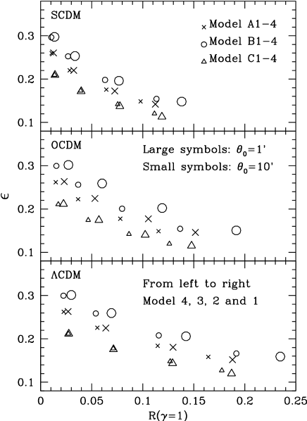
Figure 9: The slopes of the $R$-$\gamma$ relation in the semi-analytic model. Coefficient $\epsilon$ as defined in equation (10) is shown as a function of $R(\gamma=1)$.

Finally, we examine the dependence of the SLC effect on the evolution of bias. Figure 8 shows $R$ as a function of $\gamma$ for 4 models selected arbitrarily. For each source distribution model, the $R$-$\gamma$ relation is well fitted by the following empirical law,

$$\log R=\epsilon\gamma+\mbox{const}.$$ (10)

The coefficient $\epsilon$, which describes the strength of dependence of the SLC effect on the evolution of bias, is shown in Fig. 9 as a function of $R(\gamma=1$) for all source distribution models we consider. Each panel corresponds to a given choice of cosmology. One can see that $\epsilon$ remains in the range $0.1<\epsilon<0.3$ and is almost insensitive to both smoothing scale and cosmology. At a fixed value of $R(\gamma=1)$, $\epsilon$ increases with the mean redshift (in order of C, A and B). This is a natural consequence of the fact that, for our choice of the bias evolution model eq. (7), the impact of the change in the bias evolution is more significant at a higher redshift.

The uncertainty in parameter $R$ caused by our ignorance of $b(z)$ can be roughly estimated using the empirical relation (10) as follows: suppose that the power-law model (7) for the evolution of bias stands, but that there is an error $\Delta_{\gamma}$ on the value of $\gamma$. Applying simple error propagation technique, one finds $\delta R/R=2.3\,\epsilon\,{\Delta_{\gamma}}(\sim 0.5\Delta_{\gamma})$: if one is able to constrain the bias evolution model with an accuracy better than $\Delta_{\gamma}<0.4$, the uncertainty in $R$ drops below 20 per cent.

6 Testing semi-analytic predictions against numerical simulations

In this section, we compare theoretical predictions to ray-tracing experiments in $N$-body simulations, using mock galaxy catalogues extracted from the simulations as distributions of sources. The $N$-body data sets and the ray-tracing method used for this work are described in Appendix B. In Appendix C, details of the procedure to generate mock galaxy catalogues are presented. We focus only on the SCDM model, but the conclusions of our numerical analysis should not depend significantly on the considered cosmology.

Figure 10: $S_{3}$ (upper panel) and $R$ (lower panel) as functions of the smoothing angle $\theta$ in the $\gamma=0$ case. The solid (dotted) line shows the semi-analytic prediction with (without) the SLC effect taking into account, while the filled circles (triangles) show the results of ray-tracing simulations with (without) SLC effect taking into account. Error bars give some estimate of the uncertainty $E$ on the measurements, i.e. $E(S_{3})\simeq\Delta S_{3}/\sqrt{40}$, where $(\Delta S_{3})^{2}$ is the dispersion over the 40 realizations. Note that $R$ is calculated as $R=-S_{3}^{\rm slc}/S_{3}^{\rm n.l.}$, where $S_{3}^{\rm n.l.}$ is always given by semi-analytic predictions.

We measure convergence statistics on mock galaxy catalogues as follows: the value of convergence for a galaxy at redshift $z$ is given by linear interpolation between the $\kappa_{i}$ —computed from rays propagating between redshift $z$ of the closest lens plane to the galaxy (see Appendix B) and present time— measured at the four nearest angular pixels from the galaxy position in the sky. The amplitude of the SLC effect is measured by comparing simulations to similar SLC-free ones. They are obtained from other mock galaxy catalogues with the same source distribution $n_{s}(z)$ (i.e. the same as in the SLC mock catalogue), in which galaxies are randomly distributed on the sky. Note finally that top hat filtering is used and the intrinsic ellipticity of galaxies is not taken into account.

The upper panel of Fig. 10 shows the skewness parameter measured from the $\gamma=0$ mock galaxy catalogue with and without the SLC effect. The lower panel displays the function $R(\theta)$, except that in the denominator of equation (8), we always take the value given by nonlinear semi-analytic predictions, $S_{3}^{\rm n.l.}$. As discussed in Appendix B (see also Hamana & Mellier 2001), the simulations have limited available dynamic range since they are contaminated by force softening and finite volume effects at small and large scales respectively, where the measured $S_{3}$ is expected to underestimate the real value. Furthermore, there is a 10-20 per cent uncertainty in the nonlinear perturbation theory predictions. With these elements in mind, we see that agreement between measurements and predictions is reasonable when SLC effects are taken into account. In particular, the order of magnitude of the shift between the upper and the lower symbols in the top panel of Fig. 10 matches very well that between the dotted and the solid curve, as illustrated by bottom panel.

Similar results are obtained for the $\gamma=1$ and $2$ catalogues, as summarized in Fig. 11, which concentrates on the parameter $R$. Since numerical experiments for $\gamma=1$ and 2 cases are done with threshold bias instead of the linear bias used in the semi-analytic computation, we should only focus on the differences among the three models arising from different evolution of biasing. Although there is a systematic difference between the predictions and measurements, a trend in the dependence of evolution of biasing on the SLC effect found in the predictions is well reproduced in the measurements.

Furthermore, one finds that the $\gamma=2$ measurement agrees better with the $\gamma=3$ prediction except for the largest angular scales. This is consistent with the scale dependence of biasing detected in the $\gamma=2$ mock catalogue (on small scales the bias evolves as $\gamma=3$, see Appendix C for detailed discussion on this point). We may conclude from the results above that the semi-analytic approach gives a good prediction of the SLC effect on the convergence skewness.

Figure 11: The parameter $R$ as displayed in the lower panel of Fig. 10 but now for all values of $\gamma$ considered. Symbols show the results of ray-tracing simulations: circles, triangles and squares correspond respectively to $\gamma=0$, $1$ and $2$ mock catalogues. Lines correspond to semi-analytical predictions, $\gamma=0$, 1, 2, 3 from bottom to top. Error bars are computed as explained in caption of Fig. 10.

7 Summary and discussion

We have examined the source-lens clustering (SLC) effect on measurements of the skewness of lensing convergence using a nonlinear semi-analytic approach. The result of semi-analytic predictions were tested against numerical simulations, and a good agreement between them was found. Our main conclusions are as follows:

• SLC effect strongly depends on the redshift distribution of source galaxies. We found that the effect scales with the width and mean redshift of the distribution roughly as $R\propto\langle z\rangle^{-(3.0-1.8)}\Delta z^{1.4-2.5}$, (where $R=-S_{3}^{\rm slc}/S_{3}$, and $S_{3}^{\rm slc}$ is the change in measured $S_{3}$ due to SLC). As illustrated by Fig. 7, this relation indicates that it is essential to make the width of the distribution narrow and its mean redshift high to reduce the SLC effect (this was partly pointed out by B98).

• SLC effect also depends on the evolution of the bias between the galaxy and total matter distributions, $b(z)$. Assuming a simple power-law model and linear bias, $b(z)\propto(1+z)^{\gamma}$, we found that the uncertainty in $\gamma$ transforms into $\delta R/R=2.3\,\epsilon\,\Delta_{\gamma}$ with a typical value of $\epsilon\sim 0.2$. This indicates that the uncertainty in $\gamma$ must be $\Delta_{\gamma}<0.2$ for predicting the amplitude of the SLC effect with better than 10 per cent accuracy.

The main uncertainty in semi-analytic predictions comes from the fact that the accuracy of the nonlinear fitting formula of the density bispectrum is only 10-20 per cent. We expect the same level of uncertainty in predictions presented in this paper for the SLC effect on the convergence skewness. This can actually be improved by measurements in large $N$-body simulations with high spatial resolution.

Since, so far, little is known about the evolution of the bias, it is still very difficult to predict the SLC effect accurately. It is therefore very important to reduce this effect as much as possible by controlling the redshift distribution of sources. The above results tells us that an ideal observational strategy might be as follows: (i) going to a deep limiting magnitude to increase the mean redshift of the survey and (ii) using only fainter images to reduce the width of the distribution. A desirable source distribution for $R<0.1$ suggested by Fig. 7 would have $\Delta z<0.3$ and $\langle z\rangle>1$. This may be of course challenging: going to deeper magnitudes will make the calculation of the redshift distribution of sources more difficult, and using only faint images will increase the noise due to intrinsic ellipticity of galaxies. We leave more detailed studies on the designing of optimal strategies to future works.

Before closing this paper, it is important to emphasize that the use of source galaxies with a small redshift width may unfortunately introduce additional skewness signal due to the intrinsic correlation of galaxy ellipticities. It was indeed suggested that the amplitude of this latter effect scales roughly as $(\Delta z)^{-1}$, although the normalization of this relation is ambiguous because of the uncertainty in the correlation between the shape of galaxies and that of their dark matter halos (Croft & Metzler 2000; Crittenden et al. 2000; Heavens, Refregier & Heymans 2000; Pen, Lee & Seljak 2000; Catelan, Kamiokowski & Blandford 2001; Hatton & Ninin 2001). However, as pointed out by Croft & Metzler (2000), intrinsic ellipticity correlations might just act as an additional source of random noise, without significantly influencing the measured value of the skewness of the convergence.

Appendix A Perturbation theory approach to the cosmic shear statistics in the presence of SLC

The expressions for the skewness of lensing convergence and the correlation term due to SLC were first derived by BvWM97 and B98, respectively, in the framework of perturbation theory. However, B98 only gave the expression for the case of an Einstein-de Sitter cosmological model and assumed power-law density power spectrum. In this Appendix, for this paper being self-contained, we re-derive the skewness terms which are valid for an arbitrary Friedmann model. We basically follow the original deviation by B98. It should be noted that the skewness corrections are not only caused by the SLC but also arise from e.g., the lens-lens coupling (BvWM97, Van Waerbeke et al 2001b) and the lensing magnification effect (Hamana 2001). In what follows, we focus on the SLC correction and are not concerned with other correction terms.

A.1 Fluctuation in a source distribution due to the source clustering

The number density of the sources at redshift $z$ and in direction $\mn@boldsymbol{\phi}$ can be written,

$$n_{s}^{\rm obs}[\chi(z),\mn@boldsymbol{\phi}]=n_{s}[\chi(z)]\left(1+\delta_{s}[\chi(z),\mn@boldsymbol{\phi}]\right),$$ (11)

where $n_{s}[\chi(z)]$ is the average number density of sources, $\delta_{s}[\chi(z),\mn@boldsymbol{\phi}]$ is their local density contrast and $\chi$ denotes the radial comoving distance. We suppose as B98 that the average source number density is normalized to unity, $\int_{0}^{\chi_{H}}d\chi n_{s}(\chi)=1$, where $\chi_{H}$ is the distance to the horizon (the normalized distribution denotes the probability distribution). Following B98, we assume that the density contrast of sources is related to the matter density contrast, $\delta$, via the linear biasing,

$$\delta_{s}(\chi,\mn@boldsymbol{\phi})=b(\chi)\delta(\chi,\mn@boldsymbol{\phi}).$$ (12)

A.2 Convergence statistics in the presence of SLC

Let us consider the measured convergence that results from averages made over many distant galaxies located at different distances. Denoting the smoothing scale by $\theta$, such an average can formally be written as,

$$\kappa_{\theta}={{\sum_{i=1}^{N_{s}}W_{\theta}(\mn@boldsymbol{\phi}_{i})\kappa_{s}(z_{i},\mn@boldsymbol{\phi}_{i})}\over{\sum_{i=1}^{N_{s}}W_{\theta}(\mn@boldsymbol{\phi}_{i})}},$$ (13)

where $W_{\theta}(x)$ denotes the weight function of the average, $N_{s}$ is the number of source galaxies, $\kappa_{s}(z_{i},\mn@boldsymbol{\phi}_{i})$ is the lensing convergence signal from a source galaxy located at redshift $z_{i}$ in a direction $\mn@boldsymbol{\phi}_{i}$ and is given by (e.g., Mellier 1999; Bartelmenn & Schneider 2001 for reviews)

$$\kappa_{s}(z,\mn@boldsymbol{\phi})={{3\Omega_{\rm m}}\over 2}{{H_{0}}\over c}\int_{0}^{\chi_{s}(z)}d\chi_{l}\,g(\chi_{l},\chi_{s})\delta(\chi_{l},\mn@boldsymbol{\phi}),$$ (14)

with

$$g(\chi_{l},\chi_{s})={{H_{0}}\over c}{{f(\chi_{l})f(\chi_{s}-\chi_{l})}\over{f(\chi_{s})a(\chi_{l})}}.$$ (15)

Here $a$ is the scale factor normalized to its present value, and $f(\chi)$ denotes the comoving angular diameter distance, defined as $f(\chi)=K^{-1/2}\sin K^{1/2}\chi$, $\chi$, $(-K)^{-1/2}\sinh(-K)^{1/2}\chi$ for $K>0$, $K=0$, $K<0$, respectively, where $K$ is the curvature which can be expressed as $K=(H_{0}/c)^{2}(\Omega_{\rm m}+\Omega_{\lambda}-1)$. For the weight function, the angular top-hat filter (BvWM97) and/or compensated filter (Schneider et al. 1998) are commonly adopted (e.g., Van Waerbeke et al. 2001a). In what follows, we consider the top-hat filter for the weight function, and in this case equation (13) is reduced to $\kappa_{\theta}=\sum_{i=1}^{N_{s}^{j}}\kappa_{s}(z_{i},\mn@boldsymbol{\phi}_{i})/N_{s}^{j}$, where $N_{s}^{j}$ is the number of source galaxies within an aperture $\theta$ centered on a direction $\mn@boldsymbol{\phi}_{j}$. The number density of sources for current and future weak lensing analyses is about 40 per arcmin² (e.g., Van Waerbeke et al. 2001a), which typically implies more than 100 galaxies in discs of radius $\theta\geq 1$ arcmin. As a result, discreteness effects from the source distribution can be neglected (see also B98) and we can rewrite (13) in the continuous limit:

$$\kappa_{\theta}={{\int d^{2}\phi\,W_{\theta}(\mn@boldsymbol{\phi})\int_{0}^{\chi_{H}}d\chi\,\kappa_{s}(\chi,\mn@boldsymbol{\phi})n_{s}^{\rm obs}(\chi,\mn@boldsymbol{\phi})}\over{\int d^{2}\phi\,W_{\theta}(\mn@boldsymbol{\phi})\int_{0}^{\chi_{H}}d\chi\,n_{s}^{\rm obs}(\chi,\mn@boldsymbol{\phi})}}.$$ (16)

Let us now expand equation (16) in terms of $\delta$ using the perturbation theory approach, following BvWM97. The presence of SLC does not change the expression of the first order term,

$$\kappa_{\theta}^{(1)} = {{3\Omega_{\rm m}}\over 2}{{H_{0}}\over c}\int d^{2}\phi\,W_{\theta}(\mn@boldsymbol{\phi})\int_{0}^{\chi_{H}}d\chi_{s}\,{n_{s}(\chi_{s})}$$ (17)

$$\times\int_{0}^{\chi_{s}}d\chi_{l}\,g(\chi_{l},\chi_{s})\delta^{(1)}(\chi_{l},\mn@boldsymbol{\phi})$$

$$= {{H_{0}}\over c}\int d^{2}\phi\,W_{\theta}(\mn@boldsymbol{\phi})\int_{0}^{\chi_{H}}d\chi_{l}\,w(\chi_{l})\delta^{(1)}(\chi_{l},\mn@boldsymbol{\phi}),$$

where $w(\chi)$ is so-called the lensing efficiency function defined by

$$w(\chi_{l})={{3\Omega_{\rm m}}\over 2}\int_{\chi_{l}}^{\chi_{H}}d\chi_{s}g(\chi_{l},\chi_{s}){n_{s}(\chi_{s})}.$$ (18)

The second order convergence consists of two terms: one comes from the second order density perturbation and it is formally written by replacing the subscript ⁽¹⁾ in the first order expression (17) with ⁽²⁾ (BvWM97); the other one is due to SLC,

$$\kappa_{\theta}^{\rm slc(2)} = {{3\Omega_{\rm m}}\over 2}{{H_{0}}\over c}\int d^{2}\phi\,W_{\theta}(\mn@boldsymbol{\phi})$$ (19)

$$\times\int_{0}^{\chi_{H}}d\chi\,{n_{s}(\chi)}b(\chi)\delta^{(1)}(\chi,\mn@boldsymbol{\phi})$$

$$\times\int_{0}^{\chi}d\chi^{\prime}\,g(\chi^{\prime},\chi)\delta^{(1)}(\chi^{\prime},\mn@boldsymbol{\phi})$$

$$-\kappa_{\theta}^{(1)}\int d^{2}\phi\,W_{\theta}(\mn@boldsymbol{\phi})$$

$$\times\int_{0}^{\chi_{H}}d\chi\,{n_{s}(\chi)}b(\chi)\delta^{(1)}(\chi,\mn@boldsymbol{\phi}).$$

Using the small angle approximation (Kaiser 1992), equation (17) is rewritten in terms of the Fourier transform of the density contrast, $\delta(k)$, as

$$\kappa_{\theta}^{(1)} = {{H_{0}}\over c}\int_{0}^{\chi_{H}}d\chi\,w(\chi)\int{{d^{3}k}\over{(2\pi)^{3}}}\delta^{(1)}[\mn@boldsymbol{k};\chi]\exp[ik_{\chi}f(\chi)]$$ (20)

$$\times W[f(\chi)k_{\perp}\theta],$$

where the wave vector $\mn@boldsymbol{k}$ is decomposed into the line-of-sight component $k_{\chi}$ and its perpendicular, $\mn@boldsymbol{k_{\perp}}$, and $W(x)$ is the Fourier transform of the weight function. In the case of the top-hat filter, $W(x)=2J_{1}(x)/x$ where $J_{1}$ is the Bessel function of first order. In the same manner, equation (19) reads

$$\kappa_{\theta}^{\rm slc(2)} = {{3\Omega_{\rm m}}\over 2}{{H_{0}}\over c}\int_{0}^{\chi_{H}}d\chi\,{n_{s}(\chi)}b(\chi)\int_{0}^{\chi}d\chi^{\prime}\,g(\chi^{\prime},\chi)$$

$$\times\int{{d^{3}k}\over{(2\pi)^{3}}}\delta^{(1)}[\mn@boldsymbol{k};\chi]\exp[i{k}_{\chi}f(\chi)]$$

$$\times\int{{d^{3}k^{\prime}}\over{(2\pi)^{3}}}\delta^{(1)}[\mn@boldsymbol{k^{\prime}};\chi^{\prime}]\exp[i{k^{\prime}}_{\chi}f(\chi^{\prime})]$$

$$\times W[|f(\chi)\mn@boldsymbol{{k}_{\perp}}+f(\chi^{\prime})\mn@boldsymbol{{k^{\prime}}_{\perp}}|\theta]$$

$$-\kappa_{\theta}^{(1)}\int_{0}^{\chi_{H}}d\chi\,{n_{s}(\chi)}b(\chi)$$

$$\times\int{{d^{3}k}\over{(2\pi)^{3}}}\delta^{(1)}[\mn@boldsymbol{k};\chi]\exp[i{k}_{\chi}f(\chi)]W[f(\chi){k}_{\perp}\theta].$$

The average of the convergence is not affected by the presence of the SLC and is therefore zero, $\langle\kappa\rangle=0$. The variance is not affected by it either at linear order and is given by

$$V_{\kappa}(\theta) = \langle{\kappa_{\theta}^{(1)}}^{2}\rangle$$ (22)

$$= \left({{H_{0}}\over c}\right)^{2}\int_{0}^{\chi_{H}}d\chi_{l}\,w^{2}(\chi_{l})I_{0}(\chi_{l},\theta),$$

with

$$I_{0}(\chi,\theta)={1\over{2\pi}}\int dk\,kP_{\rm lin}(\chi,k)W_{\rm 2D}^{2}[kf(\chi)\theta],$$ (23)

where $P_{\rm lin}[\chi(z),k]$ is the linear density power spectrum. In the presence of SLC, the skewness parameter, defined by $S_{3}(\theta)=\langle\kappa_{\theta}^{3}\rangle/V_{\kappa}^{2}(\theta)$, consists of two terms: one comes from the second order perturbation (BvWM97),

$$\langle\kappa_{\theta}^{3}\rangle^{q.l.} = 3\langle{\kappa_{\theta}^{(1)}}^{2}\kappa_{\theta}^{(2)}\rangle$$ (25)

$$= 6\left({{H_{0}}\over c}\right)^{3}\int_{0}^{\chi_{H}}d\chi\,w^{3}(\chi)$$

$$\times\left[{6\over 7}I_{0}^{2}(\chi,\theta)+{1\over 4}I_{0}(\chi,\theta)I_{1}(\chi,\theta)\right],$$

where

$$I_{1}(\chi,\theta)={1\over{2\pi}}\int dk\,k^{2}P_{\rm lin}(\chi,k){{dW_{\rm 2D}^{2}[kf(\chi)\theta]}\over{dk}}.$$ (26)

The other arises from SLC,

$$\langle\kappa_{\theta}^{3}\rangle^{\rm slc} = 3\langle{\kappa_{\theta}^{(1)}}^{2}\kappa_{\theta}^{\rm slc(2)}\rangle$$

$$= 9\Omega_{\rm m}\left({{H_{0}}\over c}\right)^{3}\int_{0}^{\chi_{H}}d\chi\,{n_{s}(\chi)}b(\chi)w(\chi)I_{0}(\chi)$$

$$\times\int_{0}^{\chi}d\chi^{\prime}\,g(\chi^{\prime},\chi)w(\chi^{\prime})I_{0}(\chi^{\prime})$$

$$-6V_{\kappa}(\theta){{H_{0}}\over c}\int_{0}^{\chi_{H}}d\chi\,{n_{s}(\chi)}b(\chi)w(\chi)I_{0}(\chi).$$

To derive the last expression, we used an approximation, which turns out to be very accurate for top-hat smoothing (see B98 for details),

$${1\over{2\pi}}\int_{0}^{2\pi}d\vartheta\sin\vartheta W(|\mn@boldsymbol{k}+\mn@boldsymbol{k^{\prime}}|)\simeq W(k)W(k^{\prime}),$$ (28)

where $\vartheta$ is the angle between the wave vectors $\mn@boldsymbol{k}$ and $\mn@boldsymbol{k^{\prime}}$ and $k=|\mn@boldsymbol{k}|$.

Then, the convergence skewness simply reads, in the second order perturbation theory framework, $S_{3}(\theta)=S_{3}^{\rm q.l.}+S_{3}^{\rm slc}=\langle\kappa_{\theta}^{3}\rangle^{\rm q.l.}/V^{2}_{\kappa}(\theta)+\langle\kappa_{\theta}^{3}\rangle^{\rm slc}/V^{2}_{\kappa}(\theta)$, where all the terms are computed above.

Note that our calculation is slightly different from that of B98. Indeed B98 assumed an optimally weighted estimator for the convergence leading to eq. (9) of his paper instead of our eq. (16). However, with approximation (28), both estimators give the same results: eq. (A.2) would match eq. (22) of B98, and therefore we would easily recover eq. (29) of B98 for a scale-free power-spectrum.

Appendix B A brief description of the ray-tracing simulations

In this Appendix, we describe the $N$-body data sets and the ray-tracing method used for this work. More technical details are presented in Hamana & Mellier (2001).

Light ray trajectories are followed through large $N$-body simulations data set generated with a fully vectorized and parallelized Particle-Mesh (PM) code. Each $N$-body experiment involves $256^{2}\times 512$ particles in a periodic rectangular box of size $(L,L,2L)$. The mesh used to compute the forces was $256^{2}\times 512$. A light-cone of the particles was extracted from each simulation during the run as explained in Hamana, Colombi & Suto (2001). Our aim was for the light-cone to cover a large redshift range, $0\leq z\la 3$, and a field of view of $5\times 5$ square degrees. To do that, we adopted the tiling technique first proposed by White & Hu (2000): we performed 11 independent simulations covering adjacent redshift intervals $[z_{i}^{\rm min},z_{i}^{\rm max}]$, $i=1,\ldots,11$. The size of each simulation is such that the portion of the light-cone in $[z_{i}^{\rm min},z_{i}^{\rm max}]$ (aligned with the third axis) exactly fits the box-size. This way, angular resolution is approximately conserved as a function of redshift, except close to the observer. Finally, in order to have enough structures in each box, we impose the supplementary constraint $L\geq 80h^{-1}$ Mpc. As a result, $L$ follows the following sequence with redshift, $80,80,80,80,80,120,160,240,320,480,640\ h^{-1}$ Mpc.

The multiple lens-plane algorithm was used for ray-tracing calculations (Jain et al. 2000 and references therein). The lens planes (which are, at the same time, source planes) are separated by intervals of $80h^{-1}$Mpc, amounting to a total number of 38 in the redshift range $0\leq z\la 3$. For each ray, the lensing magnification matrix is computed on the source planes and is stored. We performed 40 realizations of the underlying density field by random shifts of the simulation boxes in the $(x,y)$ plane. For each realization, $512^{2}$ rays are traced backward from the observer. The initial ray directions are set on $512^{2}$ grids, which correspond to pixels of angular size $5^{\circ}/512\sim 0.59$ arcmin.

Figure 12: The skewness $S_{3}$ of the lensing convergence measured from the ray-tracing simulations (symbols) compared with nonlinear predictions (solid lines) for single source redshifts $z_{s}\sim 1$ (top), $2$, and $3$ (bottom).

Before using realistic redshift distribution of sources, we compute the skewness of the lensing convergence for single source planes, i.e., $n_{s}(z)=\delta_{D}(z=z_{s})$ where $\delta_{D}$ is the Dirac delta function. At this stage, we do not take into account the SLC effect. Figure 12 shows $S_{3}$ obtained from the simulations compared to nonlinear predictions. Measurements match theory reasonably well, as expected (Van Waerbeke et al. 2001b). There are slight differences which can be explained as follows:

1. The $N$-body simulations have a finite spatial resolution, which implies a flattening of $S_{3}$ at scales smaller than about 4 arcmin.

2. At large angular scales, $\theta\ga 20-40$ arcmin, depending on the source redshift considered (Hamana & Mellier 2001), the measured $S_{3}$ underestimates the real value, due to finite volume effects (i.e. the lack of the large scale power, which contributes to the skewness on smaller scales, due to the finite size of the simulation boxes, e.g., Colombi, Bouchet & Schaeffer 1994; see also Seto 1999).

3. There is an uncertainty in the fitting formula of the density bispectrum (section 3), which transforms into a 10-20 per cent error on the semi-analytic prediction for $S_{3}$. The differences between theory and measurements in Fig. 12 are smaller than this expectation, at least in the range where the measurements are reliable, $4\la\theta\la 20-40$ arcmin (derived from the above discussion on spatial resolution and finite volume effects). It is important to note this range is not equal to the dynamical range that the ray-tracing simulation originally have, which is much wider (see Hamana & Mellier 2001 for discussion on this point).

In conclusion, without SLC effects (yet) taken into account, the semi-analytic prediction obtained for $S_{3}$ is accurate (Van Waerbeke et al. 2001b).

Appendix C Procedure to generate mock galaxy catalogues

We generated three mock galaxy catalogues with galaxy number counts $n_{\rm s}(z)$ derived from the semi-analytic model by Devriendt & Guiderdoni (2000) and reproducing as well as possible the power-law model for the function $b(z)$, $b(z)=(1+z)^{\gamma}$ with $\gamma=0$, 1, and 2. They are extracted from exactly the same dark matter distributions as the ones used for the ray-tracing simulations.

The procedure to create the mock catalogues can be described as follows:

1. We adopt threshold biasing, i.e. for a smooth density distribution of dark matter, we assume that galaxies lie in regions of density contrast larger than some threshold which may eventually depend on redshift [point (ii) below], $\delta\geq\delta_{\rm TH}(z)$. Inside these regions, the local number density of galaxies at position $(z,\theta,\phi)$, (where $z$ denotes the redshift and $(\theta,\phi)$ denote the direction in the sky) is proportional to dark matter density

   $$n_{\rm g}(z,\theta,\phi)=\mu(z)[1+\delta(z,\theta,\phi)].$$ (29)

   The normalization factor $\mu(z)$ is such that the redshift distribution of galaxies reproduces (in terms of an ensemble average) some prior, $n_{\rm s}(z)$, discussed in (iii). To estimate the local density contrast from our discrete dark-matter particle distribution, we use local adaptive smoothing: the mean quadratic distance $d$ between each simulation particle and its 6 nearest neighbors is computed, $d^{2}=\sum_{i=1}^{6}d_{i}^{2}$ where $d_{i}$ is the separation between a central particle and $i$-the nearest neighbors. Then, $1+\delta\propto d^{-3}$. For each dark matter particle in regions with $\delta>\delta_{\rm TH}$, $N$ galaxies are randomly placed in the sphere of radius $d$ centered on the particle position. $N$ is computed from a random realization of a Poisson distribution with average ${\bar{N}}=(4/3)\pi d^{3}n_{\rm g}$, where $n_{\rm g}$ is the mean number density of galaxies.

2. Function $\delta_{\rm TH}(z)$ is determined numerically so that the measured variances of density fluctuations in a sphere of radius $8h^{-1}$ Mpc in the galaxy and the dark matter distribution, respectively $\sigma_{8}^{\rm gal.}$ and $\sigma_{8}$, satisfy

   $${{\sigma_{8}^{\rm gal.}(z)}\over{\sigma_{8}(z)}}=b(z).$$ (30)

   To do that, we use snapshots of the simulations at various redshifts $z_{i}$, and compute iteratively $\delta_{\rm TH}(z_{i})$ to match equation (30) within a 3 per cent accuracy. Then function $\delta_{\rm TH}(z)$ is obtained by linear interpolation of the $\delta_{\rm TH}(z_{i})$. Note that since for $\gamma=0$, $b=1$ irrespective of the redshift, the galaxy distribution directly traces the matter distribution, and thus we do not need to have threshold i.e., we simply set $\delta_{\rm TH}=\delta_{\rm min}-1$.

3. A prior function $n_{s}(z)$ is needed to compute the normalization factor $\mu(z)$ equation (29). We have used the ab-initio semi-analytic approach to galaxy formation described in Devriendt & Guiderdoni (2000) to obtain a reasonably realistic estimate of this function. Such an approach is based on a Press–Schechter like prescription to compute the number of galaxies as a function of redshift, coupled to spectro-photometric evolution of stellar populations to calculate their luminosities. The results naturally match observed galaxy number counts and redshift distributions, as well as the diffuse extragalactic background light for wavelengths ranging from the $UV$ to the near $IR$. Here, we suppose that galaxies are selected in the $I$ band, down to the magnitude $I_{AB}=24.5$. As a result, the final mock catalogues yields a typical surface number density of 29 sources per arcmin² distributed in redshift as shown in Figure 13. The distribution has a peak at $z\sim 0.4$, with mean redshift $\langle z\rangle\sim 0.8$ and typical width $\Delta z\sim 0.6$.

Note that, for $b>1$, the linear bias prescription breaks down, because $\delta_{s}$ can not be less than $-1$ by definition (in the perturbation theory approach, this does not cause a serious problem because $|\delta|$ is supposed to be much less than unity). Therefore, we do not take the linear bias but use the threshold bias for the cases of $\gamma=1$ and 2. Accordingly, strictly speaking, the direct comparison between the semi-analytical prediction and the numerical simulation makes sense only for the $\gamma=0$ model. However, we take $\gamma=1$ and 2 models to test the effect of the redshift evolution of bias which should not depend strongly on details of the biasing prescription. Moreover, to test the robustness of semi-analytic predictions in which the simple linear bias is used, it is interesting to use a different biasing prescription for the numerical experiments.

Figure 13: The distribution of sources (histogram with error bars) and the lensing efficiency function (dotted line) as functions of redshift. Error bars denote standard deviation computed among 40 realizations as discussed in Appendix B.

Figure 14: The biasing function ${\tilde{b}}$ [equation (31)] as a function of spatial scale $\ell$, measured in the mock galaxy catalogues. The top and bottom panels correspond respectively to $\gamma=1$ and $\gamma=2$ (by construction, we exactly have ${\tilde{b}}=1$ for $\gamma=0$). Each curve is for a fixed value of $z$, namely $z\simeq 0.18$, $0.33$, $0.62$, $1.25$ and $2.70$ from bottom to top of each panel. On the top panel, the squares and the triangle give the values expected from $b(z)=1+z$. On the bottom panel, the square and the triangle correspond respectively to $b(z)=(1+z)^{3}$ and $b(z)=(1+z)^{2}$.

Figure 14 shows the scaling behavior of the bias factor defined by

$${\tilde{b}}(z,\ell)\equiv\frac{\sigma_{\rm gal.}(\ell,z)}{\sigma(\ell,z)},$$ (31)

as measured in the mock catalogues with $\gamma=1$ and $\gamma=2$. In this equation, $\sigma_{\rm gal.}^{2}(\ell)$ and $\sigma^{2}(\ell)$ are respectively the variances in a sphere of radius $\ell$ of the galaxy and the matter density distribution. In fact, we take for $\sigma^{2}$ the variance measured in the mock catalogue with $\gamma=0$ which is unbiased by definition. To correct for variations of the selection function we use the method proposed by Colombi, Szapudi & Szalay (1998). The curves on each panel correspond to redshift slices of $[0.16,0.20]$, $[0.3,0.36]$, $[0.56,0.68]$, $[1.09,1.41]$ and $[2.40,3.00]$.

By construction, the value of ${\tilde{b}}$ measured at $\ell=8^{-1}$Mpc (triangles) matches very well relation (30). However there is no guarantee for this result to hold at all scales. In other words, at fixed $z$, function ${\tilde{b}}(\ell,z)$ is not necessarily a constant of scale [and equal to $b(z)=(1+z)^{\gamma}$], although this is pretty much the case for the $\gamma=1$ mock catalogue.

For the $\gamma=2$ mock catalogue, function ${\tilde{b}}(\ell,z)$ presents large variations with scale, increasing with redshift. This can be modeled as a varying effective ${\tilde{\gamma}}(\ell)$, for example ${\tilde{\gamma}}\simeq 3$ for $\ell=1h^{-1}$ Mpc (squares on bottom panel of Fig. 14). While converting scales to angles, more relevant to our analysis, the modeling in terms of a function ${\tilde{\gamma}}(\theta)$ is not very convincing. Still, we find that in the range of interest, $4\la\theta\la 20-30$ arcmin, we should compare measured SLC effects to semi-analytic predictions corresponding to $2\la\gamma\la 3$.

References

- [1] Bacon D., Refregier A., Ellis. R., 2000, MNRAS, 318, 625
- [2] Bartelmann M., Schneider P., 2001, Physics Report, 340, 291
- [3] Bernardeau F., 1998, A&A, 338, 375 (B98)
- [4] Bernardeau F., Van Waerbeke L., Mellier Y., 1997, A&A, 322, 1 (BvWM97)
- [5] Bond J. R., Efstathiou, G., 1984, ApJ, 285, L45
- [6] Catelan P., Kamionkowski M., Blandford R. D., 2001, MNRAS, 320, L7
- [7] Colombi S., Bouchet F. R., Schaeffer R., 1994, A&A, 281, 301
- [8] Colombi S., Szapudi I., Szalay A.S., 1998, MNRAS, 296, 253
- [9] Crittenden R. G., Natarajan P., Pen U.-L., Theuns T., 2001, ApJ, 559, 552
- [10] Croft R. A. C., Metzler C. A., 2001, ApJ, 545, 561
- [11] Devriendt J. E. G., Guiderdoni B., 2000, A&A, 363, 851
- [12] Eke V. R., Cole S., Frenk C. S., 1996, MNRAS, 282, 263
- [13] Hamana T., 2001, MNRAS, 326, 326
- [14] Hamana T., Colombi S., Suto Y., 2001, A&A, 367, 18
- [15] Hamana T., Mellier Y., 2001, MNRAS, 327, 169
- [16] Hatton S., Ninin S., 2001, MNRAS, 322, 576
- [17] Heavens A., Refregier A., Heymans C., 2000, MNRAS, 319, 649
- [18] Jain B., Seljak U., 1997, ApJ, 484, 560
- [19] Jain B., Seljak U., White S. D. M., 2000, ApJ, 530, 547
- [20] Jenkins A., et al. (The Virgo consortium), 1997, ApJ, 499, 20
- [21] Kaiser N., 1992, ApJ, 388, 272
- [22] Kaiser N., 1998, ApJ, 498, 26
- [23] Kaiser N., Wilson G., Luppino G. A., 2000, ApJ submitted (astro-ph/0003338)
- [24] Kitayama T., Suto Y., 1997, ApJ, 490, 557
- [25] Maoli R., et al., 2001, A&A, 368, 766
- [26] Mellier Y., 1999, ARA&A, 37, 127
- [27] Peacock J. A., Dodds, S. J., 1996, MNRAS, 280, L19
- [28] Pen U.-I., Lee J., Seljak U., 2000, ApJ, 543, L107
- [29] Schneider P., Van Waerbeke L., Jain B., Kruse G., 1998, MNRAS, 296, 873
- [30] Scoccimarro R., Couchman H. M. P., 2001, MNRAS, 325, 1312
- [31] Seto N., 1999, ApJ, 523, 24
- [32] Thion A., Mellier Y., Bernardeau F., Bertin E., Erben T., Van Waerbeke L., 2001, Proceedings of the XXth Moriond Astrophysics Meeting ”Cosmological Physics with Gravitational Lensing”, eds. J.-P. Kneib, Y. Mellier, M. Moniez and J. Tran Thanh Van (EDP Sciences, Les Ulis), p. 191 (astro-ph/0008180)
- [33] Van Waerbeke L., Bernardeau F., Mellier Y., 1999, A&A, 342, 15
- [34] Van Waerbeke L., et al., 2000, A&A, 358, 30
- [35] Van Waerbeke L., et al., 2001a, A&A, 375, 757
- [36] Van Waerbeke L., Hamana T., Scoccimarro R., Colombi S., Bernardeau F., 2001b, MNRAS, 322, 918
- [37] White. M., Hu W., 2000, ApJ, 537, 1
- [38] Wittman D. N., et al., 2000, Nature, 405, 143