CMB anisotropy from spatial correlations of clusters of galaxies

Abstract

The Sunyaev-Zel’dovich (SZ) effect from clusters of galaxies is a dominant source of secondary cosmic microwave background (CMB) anisotropy in the low-redshift universe. We present analytic predictions for the CMB power spectrum from massive halos arising from the SZ effect. Since halos are discrete, the power spectrum consists of a Poisson and a correlation term. The latter is always smaller than the former, which is entirely dominated by nearby bright massive halos, i.e., by rich clusters. In practice however, those bright clusters are easy to indentify and can thus be subtracted from the map. After this subtraction, the correlation term dominates degree-scale fluctuations over the Poisson term, as the main contribution to the correlation term comes from distant clusters. We compare the signal of the correlation term to the expected sensitivity for the Planck experiment for the SZ effect, and find that the correlation term is detectable. Since the degree scale spectrum is quite insensitive to the highly uncertain core structures of halos, our predictions are robust on these scales. Measuring the correlation term on degree scales thus cleanly probes the clustering of distant halos. This has not been measured yet, mainly because optical and X-ray surveys are not sufficiently sensitive to include such distant clusters and groups. Our analytic predictions are also compared to adiabatic hydrodynamic simulations. The agreement is remarkably good, down to ten arcminutes scales, indicating that our predictions are robust for the Planck experiment. Below ten arcminute scales, where the details of the core structure dominates the power spectrum, our analytic and simulated predictions might fail. In the near future, interferometer and bolometer array experiments will measure the SZ power spectrum down to arcminutes scales, and yield new insight into the physics of the intrahalo medium.

1 Analytic halo approach to the power spectrum

We construct an analytic model of the power spectrum of the cosmic microwave background (CMB) anisotropy arising from halos through the Sunyaev-Zel’dovich (SZ) effect. Since halos, which include clusters of galaxies, groups, and galaxies, are discrete objects, their angular power spectrum $C_{l}$ consists of a Poisson term $C_{l}^{(P)}$ and a correlation term $C_{l}^{(C)}$ that arises from their gravitational clustering[1, 2]:

$$C_{l}=C_{l}^{(P)}+C_{l}^{(C)}.$$ (1)

The following describes our prescription for computing the SZ power spectrum using the halo approach. The key ingredients in our prescription are (1) the halo mass function $dn(M,z)/dM$, (2) the halo bias parameter $b(M,z)$, and (3) the halo gas pressure profile $y(\theta)$. (1) and (2) are computed from the Press-Schechter theory[4, 5, 6], while (3) is calculated assuming that halos are virialized and isothermal. The halo approach has also been used independently to predict the non-linear dark matter power spectrum[7] and bispectrum[8]. In this case, (3) is replaced by the dark matter halo profile. These predictions are successful in reproducing the results of N-body simulations. Thus, as far as dark matter is concerned, our prescription is adequate to describe the halo-halo correlation. However, once gas dynamics is included, the degree of uncertainty in (3) increases. We will see below that our analytic prediction nevertheless agrees well with state-of-the-art hydrodynamic simulations[9, 10, 11, 12] (see figure 1).

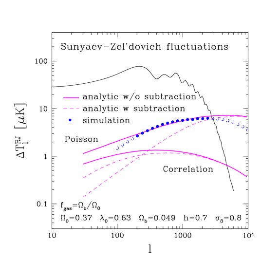
Figure 1: Power spectrum of SZ anisotropies from massive halos ($2\times 10^{12}~{}h^{-1}~{}M_{\odot}<M<2\times 10^{15}~{}h^{-1}~{}M_{\odot}$) in units of $\mu{\rm K}$ in the Rayleigh-Jeans limit. Thick solid lines show analytic predictions for the Poisson and the correlation terms, while dotted lines show the predictions after subtracting the ROSAT X-ray flux-limited samples. The number density of subtracted clusters is $0.8~{}{\rm deg^{-2}}$. Filled and open circles show the power spectrum measured from hydrodynamic simulations. Filled circles correspond to the dynamic range that is reliably resolved in the simulation.

1.1 Mass function

One of the key ingredients in our analytic prediction is the halo mass function $dn(M,z)/dM$, which we compute from the Press-Schechter formalism[4]. This formalism, which plays a central role in our method, was used by Cole and Kaiser[1] to calculate the rms SZ fluctuation from halos, including both the Poisson and the correlation terms. Makino and Suto[13] calculated the Poisson term including the effect of halo profiles, assuming the $\beta$ profile. Thanks to the recent remarkable developments of the microwave experiments, it is now feasible to measure not only the rms fluctuation but also the full CMB two point function, or its harmonic transform, the angular power spectrum $C_{l}$, very accurately down to arcminutes angular scales. Atrio-Barandela and Mücket[14] calculated $C_{l}$ from the Poisson term of SZ fluctuations using the Press-Schechter mass function and the $\beta$ profile.

1.2 Bias parameter

We predict the SZ power spectrum $C_{l}$ that includes the correlation term[3]. For this purpose, we need the halo-halo correlation function and its evolution with redshift. In the framework of the Press-Schechter theory, these can be calculated from the underlying dark matter correlation multiplied by the bias parameter $b(M,z)$[5, 6]. In Fourier space, this can be formulated, to the leading order as

$$P_{hh}(k,M_{1},M_{2},z)\simeq b(M_{1},z)b(M_{2},z)P_{dm}(k,z),$$ (2)

where $P_{hh}(k)$ and $P_{dm}(k)$ are the halo-halo and the dark matter power spectrum, respectively.

1.3 Halo profile

In predicting the power spectrum of halos, we need the halo profile which determines the small scale power. Since the SZ effect is produced from thermal gas pressure, we need to model both the gas density profile and the temperature profile. Firstly, we assume that halos are virialized objects with an isothermal temperature distribution. Then, we use observationally determined halo gas density profiles, namely the $\beta$-profile with $\beta=2/3$ and a core radius of $0.15~{}h^{-1}~{}{\rm Mpc}$ at $M=10^{15}~{}h^{-1}~{}M_{\odot}$ and $z=0$. We let the core evolve with time according to the self-similar evolution[15]. Note that the evolution of the core is the most uncertain parameter in our model. Atrio-Barandela and Mücket[14] employed a different evolution model, and found that the arcminute-scales $C_{l}$’s are sensitive to the core evolution model. We confirmed their result, and also found that the larger angular scale spectrum is fairly insensitive to the core model. Thus, as long as angular scales larger than about ten arcminutes are considered, uncertainties in core evolution model do not affect the prediction.

2 Power spectrum of the Sunyaev–Zel’dovich effect

2.1 Poisson and correlation terms

Using the harmonic transform of the $\beta$ profile for the SZ surface brightness distribution, $y_{l}(M,z)$, we get the following analytic expressions for the angular power spectrum:

$$C_{l}{}^{(P)} = j_{\nu}^{2}\int dz\frac{dV}{dz}\int dM\frac{dn(M,z)}{dM}\left|y_{l}(M,z)\right|^{2},$$ (3)

$$C_{l}{}^{(C)} = j_{\nu}^{2}\int dz\frac{dV}{dz}P_{dm}\left(\frac{l}{r(z)},z\right)\left[\int dM\frac{dn(M,z)}{dM}b(M,z)y_{l}(M,z)\right]^{2},$$ (4)

where $P$ and $C$ denote the Poisson and the correlation terms, respectively. $j_{\nu}$ is the spectral function of the Sunyaev–Zel’dovich effect and equals $-2$ in the Rayleigh–Jeans regime[16]. The range of the mass integral determines what objects are considered. We choose $2\times 10^{12}~{}h^{-1}~{}M_{\odot}<M<2\times 10^{15}~{}h^{-1}~{}M_{\odot}$, corresponding approximately to the resolution and box-size limits of our hydrodynamic simulation[9]. The redshift integral up to $z=5$ is found to be sufficient for convergence. Our choice of cosmological parameter is $\Omega_{0}=0.37$, $\lambda_{0}=0.63$, $\Omega_{b}=0.049$, $h=0.7$, and $\sigma_{8}=0.8$.

Figure 1 shows the numerical results from equations (3) and (4). Firstly, $C^{(C)}_{l}$ is always smaller than $C^{(P)}_{l}$. $C^{(P)}_{l}$ has a turn over at around $l\sim 5000$, which corresponds to the typical angular size of core radii. Since the spectrum for $l>2000$ is very sensitive to the halo core model[14, 3], it is highly uncertain. We thus mainly focus on larger angular scales ($l<2000$). Note however, that the small-scale spectrum is of great interest, as it potentially probes the intracluster gas pressure state. Although Planck cannot probe the spectrum beyond $l\sim 2000$, forthcoming interferometer and bolometer array experiments will certainly measure SZ fluctuations on these scales.

2.2 Subtracting nearby bright clusters

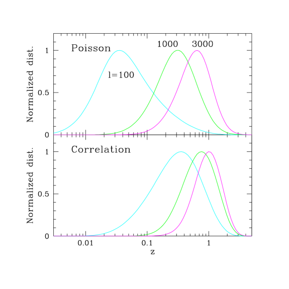
Figure 2: Redshift distribution of the SZ power spectrum in $\log z$-interval, at $l=100$, 1000, and 3000. Amplitudes are normalized to unity.

Can we measure the correlation term? Yes! Since nearby massive clusters (such as the Coma cluster) dominate the Poisson term on large angular scales, the Poisson shot noise will be substantially reduced if bright clusters are excised from the map. Figure 2 shows the redshift distribution of $C_{l}$ at 3 different angular scales, $l=100$, 1000, and 3000. Nearby halos in $z=0.01-0.1$ dominate the Poisson $C^{(P)}_{100}$, while the correlation $C^{(C)}_{100}$ come from $z=0.1-1$. This clear separation in redshift space allows us to remove the Poisson shot noise, while preserving the correlation term.

One way of doing this is to subtract a homogeneous sample of local clusters from the SZ map. Figure 1 shows the SZ power spectrum before (solid lines) and after (dashed lines) subtracting an X-ray selected cluster sample with the flux limit $>10^{-13}~{}{\rm erg~{}cm^{-2}~{}s^{-1}}$ in the ROSAT ($0.5-2$ keV) band. The Poisson spectrum is greatly reduced, while the correlation spectrum is less affected by the subtraction. The correlation term actually dominates over the Poisson term for $l<200$. The number density of subtracted clusters is $0.8~{}{\rm deg^{-2}}$. For this figure, the X-ray flux was calculated by the method of Kitayama and Suto[17]. Alternatively, one can identify bright SZ clusters in the CMB map itself, and then subtract them[3]. For example, $0.9~{}{\rm deg^{-2}}$ clusters can be removed for ones brighter than $50~{}{\rm mJy}$ at 350 GHz.

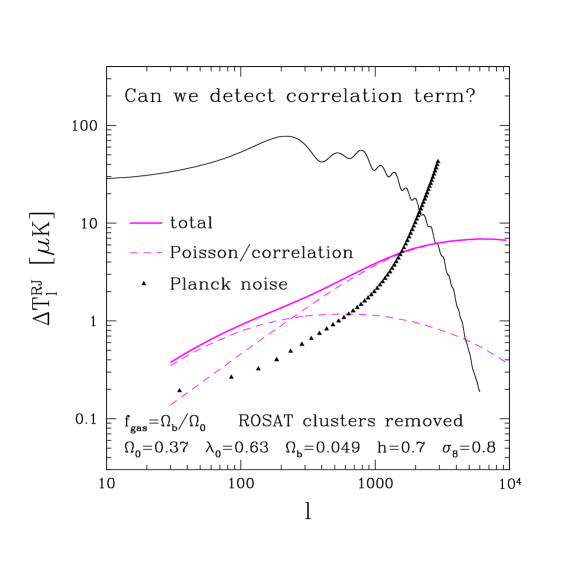
Figure 3: Comparison of the predicted signal from the correlation term to the expected sensitivity of the Planck experiment (filled triangles) to the Sunyaev-Zel’dovich effect. The noise power spectrum has been binned into bands with $\Delta l=50$. The thick solid line shows the total spectrum, while the dashed lines show the Poisson and the correlation terms separately. The ROSAT X-ray flux-limited sample was removed. The number density of subtracted clusters is $0.8~{}{\rm deg^{-2}}$. Note that the plotted sensitivity is the residual noise level after subtracting the primary CMB signal from the map, on the basis of a multi-frequency analysis.

2.3 Can we detect the correlation term?

Even if the correlation term overcomes the Poisson term, the primary CMB fluctuations may prevent us from measuring the correlation term on degree scales. Can we really measure the correlation term? Yes! Thanks to the unique shape of the frequency spectrum $j_{\nu}$ of the SZ effect[16], we can subtract the primary CMB, and hopefully other foregrounds from the map. In other words, we expect to be able to derive a cleaned SZ map. Cooray, Hu and Tegmark[18] demonstrated this technique: using the frequency separation, they obtained the expected noise level for the SZ power spectrum after subtracting the primary CMB and other modeled sources of foreground. Figure 3 compares the signal of the correlation term to the resulting SZ noise power spectrum, binned into bands with $\Delta l=50$. The result is so encouraging that we can hope to measure the contribution from the correlation term fairly accurately at $l=30-200$. Since the degree-scale spectrum is insensitive to the highly uncertain core structures of halos, our predictions are robust on these scales. Thus, measuring the correlation term cleanly probes the clustering of distant halos. Such a measurement has not been achieved yet, mainly because of the lack of sensitivity of optical and X-ray surveys to such distant clusters and groups. The fact that the SZ effect is very sensitive to high redshift, is a consequence of the known fact that the SZ surface brightness is independent of $z$.

3 Comparison to the moving-mesh hydrodynamic simulation

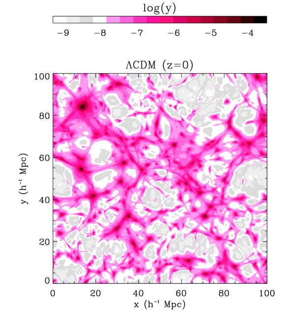
Figure 4: Snap shot of $y$-parameter in the moving-mesh hydrodynamic simulation at $z=0$. The box size is $L=100~{}h^{-1}~{}{\rm Mpc}$, and the number of cells is $N=128^{3}$. The effective spatial resolution at $z=0$ is $\sim 80~{}h^{-1}~{}{\rm kpc}$. Our choice of cosmological parameters is $\Omega_{0}=0.37$, $\lambda_{0}=0.63$, $\Omega_{b}=0.049$, $h=0.7$, and $\sigma_{8}=0.8$. The angular power spectrum of the SZ effect from the simulation is plotted in figure 1. For the simulation, the mean density-weighted temperature at present is 0.25 keV, and the mean $y$-parameter is $1.7\times 10^{-6}$, in good agreement with the Press-Schechter predictions.

We carried out adiabatic hydrodynamic simulations[9] using the moving-mesh hydrodynamic code written by Pen[19]. The code captures the advantages of both the Lagrangian particle based and the Eulerian grid based codes by allowing the grid meshes to deform along potential flow lines. This strategy makes it possible to increase the resolution by twenty fold over previous Cartesian grid Eulerian schemes, at a low computational cost.

Figure 4 shows a snap shot of the $y$-parameter in the simulation at $z=0$. The box size is $L=100~{}h^{-1}~{}{\rm Mpc}$, and the number of cells is $N=128^{3}$. Since the linear compression factor is about 10, the effective spatial resolution at $z=0$ is $\sim 80~{}h^{-1}~{}{\rm kpc}$. Our cosmological parameters are $\Omega_{0}=0.37$, $\lambda_{0}=0.63$, $\Omega_{b}=0.049$, $h=0.7$, and $\sigma_{8}=0.8$. The mass range resolved in this simulation is $2\times 10^{12}~{}h^{-1}~{}M_{\odot}<M<2\times 10^{15}~{}h^{-1}~{}M_{\odot}$.

Figure 1 compares the angular power spectrum of the SZ effect from the simulation (filled and open circles) to the analytic predictions (solid lines). The filled circles highlight the $l$-range, $200<l<2000$, which is reliably described in the simulation. The agreement between the simulation and the analytic prediction is impressively good. Likewise, the mean density weighted temperature at present is 0.25 keV, and the mean $y$-parameter is $1.7\times 10^{-6}$, in good agreement with the Press-Schechter predictions. Thus, our halo approach to the SZ effect works as long as relatively massive halos resolved in this simulation are considered. We conclude that the SZ power spectrum in $200<l<2000$ is dominated by these massive halos.

4 Discussion

Our analytic predictions agree well with the adiabatic hydrodynamic simulations; however, our halo gas pressure model disagrees somewhat with observations. This disagreement affect our analytic predictions and simulated results qualitatively on smaller angular scales, say, $l>2000$. For example, the self-similar model appears to have difficulties in explaining the X-ray luminosity–temperature relation[20], the mass–temperature relation[21], and the central entropy–temperature relation[22]. The departure from the adiabaticity due to so-called preheating is thought to be a solution to these problems. If this is so, the adiabatic simulation would not describe the intrahalo gas state accurately. The resolution of these disagreements seems to require larger core radii than those predicted by the self-similar model. This would tend to suppress the small scale power spectrum, as compared to the adiabatic case[11]. Including those effects in analytic predictions is rather challenging, but is important. Interferometer and bolometer array CMB experiments are expected to measure the SZ power spectrum accurately down to arcminutes scales, in the near future. These experiments will thus certainly further our understanding of the intracluster medium.

References

- [1] S. Cole and N. Kaiser, Mon. Not. R. Astron. Soc. 233, 637 (1988).
- [2] P. J. E. Peebles, The Large Scale Structure of the Universe (Princeton University Press, Princeton, 1980).
- [3] E. Komatsu and T. Kitayama, Astrophys. J. Lett. 526, L1 (1999).
- [4] W. H. Press and P. Schechter, Astrophys. J. 187, 425 (1974).
- [5] H. J. Mo and S. D. M. White, Mon. Not. R. Astron. Soc. 282, 347 (1996).
- [6] P. Catelan, F. Lucchin, S. Matarrese and C. Porciani, Mon. Not. R. Astron. Soc. 297, 692 (1998).
- [7] U. Seljak, Mon. Not. R. Astron. Soc. 318, 203 (2000).
- [8] C.-P. Ma and J. N. Fry, Astrophys. J. 543, 503 (2000).
- [9] A. Refregier, E. Komatsu, D. N. Spergel and U.-L. Pen, \Journal\PRD611230012000.
- [10] U. Seljak, J. Burwell and U.-L. Pen, preprint, astro-ph/0001120.
- [11] V. Springel, M. White and L. Hernquist, preprint, astro-ph/0008133.
- [12] A. C. da Silva, D. Barbosa, A. R. Liddle and P. A. Thomas, preprint, astro-ph/0011187.
- [13] N. Makino and Y. Suto, Astrophys. J. 405, 1 (1993).
- [14] F. Atrio-Barandela and J. P. Mücket, Astrophys. J. 515, 465 (1999).
- [15] N. Kaiser, Mon. Not. R. Astron. Soc. 222, 323 (1986).
- [16] Ya. B. Zel’dovich and R. A. Sunyaev, Astrophys. Space. Sci. 4, 301 (1969).
- [17] T. Kitayama and Y. Suto, Astrophys. J. 490, 557 (1997).
- [18] A. Cooray, W. Hu and M. Tegmark, Astrophys. J. 540, 1 (2000).
- [19] U.-L. Pen, Astrophys. J. Suppl. Ser. 100, 269 (1995); ibid. 115, 19 (1998).
- [20] M. Arnaud and A. E. Evrard, Mon. Not. R. Astron. Soc. 305, 631 (1999).
- [21] A. Finoguenov, T. H. Reiprich and H. Böhringer, preprint, astro-ph/0010190.
- [22] T. J. Ponman, D. B. Cannon and J. F. Navarro, Nature 397, 135 (1999).