HST STIS observations of the He II  Gunn-Peterson effect towards HE 2347–4342 (catalog )

Abstract

We present an HST STIS spectrum of the He II Gunn-Peterson effect towards HE 2347-4342 (catalog ). Compared to the previous HST GHRS data obtained by Reimers et al. (1997), the STIS spectrum has a much improved resolution. The 2-dimensional detector also allows us to better characterize the sky and dark background. We confirm the presence of two spectral ranges of much reduced opacity, the opacity gaps, and provide improved lower limits on the He II Gunn-Peterson opacity $\tau_{\mathrm{HeII}}$ in the high opacity regions. We use the STIS spectrum together with a Keck–HIRES spectrum covering the corresponding H I Ly-$\alpha$ forest to calculate a 1-dimensional map of the softness $S$ of the ionization radiation along the line of sight towards HE 2347-4342 (catalog ), where $S$ is the ratio of the H I to He II photoionization rates. We find that $S$ is generally large but presents important variations, from $\sim 30$ in the opacity gaps to a 1 $\sigma$ lower limit of 2300 at $z\simeq 2.86$, in a region which shows an extremely low H I opacity over a 6.5 Å  spectral range. We note that a large softness parameter naturally accounts for most of the large Si IV to C IV ratios seen in other quasar absorption line spectra. We present a simple model that reproduces the shape of the opacity gaps in absence of large individual absorption lines. We extend the model described in Heap et al. (2000) to account for the presence of sources close to the line of sight of the background quasar. As an alternative to the delayed reionization model suggested by Reimers et al. (1997), we propose that the large softness observed at $z\simeq 2.86$ is due to the presence of bright soft sources close to the line of sight, i.e. for which the ratio between the number of H I to He II ionizing photons reaching the intergalactic medium is large. We discuss these two models and suggest ways to discriminate between them.

1 Introduction

General considerations of the shape and intensity of the UV background and the ionization state of the intergalactic medium indicate that He⁺ is the most abundant absorbing ion in low-density regions of the Universe at $z\sim 3$ (e.g. Zheng & Davidsen, 1995; Croft et al., 1997; Miralda-Escudé, Haehnelt, & Rees, 2000). Consequently, a continuous depression of the flux of quasars (or any other sources) blueward of the He II Ly-$\alpha$ emission line is predicted. By similarity with the effect expected in H I (Gunn & Peterson, 1965; Scheuer, 1965), this depression is called the He II Gunn-Peterson effect. One can easily show that the bulk of He II opacity, $\tau_{\mathrm{HeII}}$, must originate in clouds of low H I column density, $\log{N_{\mathrm{HI}}}<13$ (Croft et al., 1997; Fardal et al., 1998); in other words, the He II Gunn-Peterson effect probes the lowest density region of the Universe, and most of its volume. Consequently, this effect allows us to probe the UV background ionizing radiation. On the other hand, spectral regions showing low He II opacity, or opacity gaps, are also expected. They may arise either as a consequence of additional ionizing sources close to the line of sight to the background quasar, in intrinsically low density regions, or in regions dominated by the presence of shock-heated gas.

The He II Gunn-Peterson effect is difficult to study observationally due to the scarcity of lines of sight towards bright quasars devoid of strong Lyman limit systems (Møller & Jakobsen, 1990; Picard & Jakobsen, 1993). Jakobsen et al. (1994) were the first to study the He II Gunn-Peterson absorption using a spectrum of the $z=3.28$ quasar Q 0302-003 (catalog ) obtained with the Faint Object Camera on the Hubble Space Telescope (HST). Using the Hopkins Ultraviolet Telescope, Davidsen, Kriss, & Zheng (1996) found $\tau_{\mathrm{HeII}}=1.00\pm 0.07$ towards HS 1700+6416 (catalog ). Q 0302-003 (catalog ) was also observed by Hogan, Anderson & Rugers (1997) with the Goddard High Resolution Spectrograph (GHRS), which revealed $\tau_{\mathrm{HeII}}>1.3$. Subsequently, Heap et al. (2000) reported on new HST STIS spectra of this quasar. The high quality of the STIS spectrum – due, in particular, to the 2-D nature of the FUV MAMA detector allowing a very good background determination – revealed regions of high opacity with $\tau_{\mathrm{HeII}}\sim 4.8$ as well as regions of low opacity, or opacity gaps, extending over several Mpc. They also presented the results of a modeling of the spectra for which the opacity is based on the redshifts, $z$, and H I column densities, $N_{\mathrm{HI}}$, defined by the observed lines in the H I Ly-$\alpha$ forest and a diffuse gas component represented by a randomly drawn sample of lines with $\log{N_{\mathrm{HI}}}<13$. They found that the high opacity regions require a diffuse gas component and a large value of $\eta\equiv N_{\mathrm{HeII}}/N_{\mathrm{HI}}\simeq 350$. In turn, this result implied that the UV background has a soft spectrum, with a softness parameter, $S\equiv\Gamma_{\mathrm{HI}}^{\mathrm{J}}/\Gamma_{\mathrm{HeII}}^{\mathrm{J}}\simeq 800$, where the $\Gamma_{i}^{\mathrm{J}}$ are the UV background photoionization rates for H I and He II, respectively. They also tested different hypotheses to explain a prominent opacity gap at $z=3.05$ and argued that it most likely arises in a region where helium is doubly ionized by a discrete local source, quite possibly an AGN.

The present paper reports on new HST STIS observations of the He II Gunn-Peterson effect towards the quasar HE 2347-4342 (catalog ). Previous HST GHRS spectra of this object obtained by Reimers et al. (1997) revealed the first evidence of a “patchy” intergalactic medium: their spectra showed (a) regions of low opacity in He II with a matching lack of absorption in H I; (b) regions of high opacity in He II at the same redshift as several H I lines; (c) regions of high opacity in He II at redshifts where no or only low column density H I lines are detected. Reimers et al. (1997) interpret theses observations as evidence that re-ionization of He II has not yet taken place, being delayed relative to H I re-ionization.

The new STIS observations provide a significant improvement in terms of signal-to-noise ratio and a more secure background determination compared to the GHRS data. The STIS spectra also have a substantially better spectral resolution. The following section, §2, summarizes the observations. Section 3 describes the spectrum and the opacity measurements. In §4, we describe how to build a one-dimensional map of the softness parameter, in a very model-independent way. In §5, we present a simple model of the opacity gaps and we expand the model described in Paper I to take into account several ionizing sources close to the line of sight to the quasar. We also discuss the possible causes of the large softness parameter seen in a large fraction of the spectral range covered by our data. In particular, we compare the delayed re-ionization model (Reimers et al., 1997) to a scenario where soft sources lead to a local increase of the UV background softness parameter. In §6, we provide a summary of the paper, and we compare our most important results with recent FUSE observations of this object (Kriss et al., 2001). Throughout this paper, we use the following cosmological parameters: $H_{\mathrm{0}}=65~{}\mbox{km}~{}\mbox{s}^{-1}~{}\mbox{Mpc}^{-1}$, $\Omega_{\mathrm{M}}=0.3$ and $\Lambda=0.7$

2 Observations

In order to improve our understanding of the He II Gunn-Peterson effect shown in the HST STIS spectra of HE 2347-4342 (catalog ), we also require good spectra covering the H I Ly-$\alpha$ forest. In this section, we describe the HST STIS and Keck–HIRES observations of this object.

2.1 HST STIS observations of the redshifted He II region.

We obtained the STIS observations of HE 2347-4342 (catalog ) in November 1998 during the course of two “visits”, each five orbits long (Program 7575). The observations used the G140M grating which produced a spectrum covering the wavelength interval 1145–1200 Å. The combined 10 exposures led to a total exposure time of 29,000s. The spectra have a resolution of 0.16 Å  FWHM, equivalent to 3 “lo-res” pixels (Woodgate et al., 1998; Kimble et al., 1998). The corresponding resolving power is $R=7,300$.

The observations were reduced at the Goddard Space Flight Center with the STIS Investigation Definition Team (IDT) version of CALSTIS (Lindler, 1998), which allowed us to make a customized treatment of the background. Such flexibility is needed in order to ensure accurate fluxes and opacities in the Gunn-Peterson trough.

The detector background in a STIS G140M observation is highly non-uniform, with a large “hot-spot” of dark counts which increases in amplitude with increasing detector temperature (see e.g. Fig. 1 of Brown et al., 2000). The QSO spectrum intersects this hot-spot roughly through the middle. Because of the non-uniformity of the background and the variation of its level from exposure to exposure, we decided to reduce and combine the spectra following the optimal extraction algorithm detailed by Robertson (1986). This method led to a significant improvement of the final S/N because it provides optimal weights to individual spectra, so that those extracted from high dark current exposures contribute proportionally less than those with low background. The only deviation from the Robertson (1986) algorithm involves the estimation of the background in each exposure, for which we used the following method. Two 50–pixel wide zones were defined above and below the QSO spectrum, both offset by 11 pixels from it. The mean intensity of the 50 pixels of each column of each zone was calculated, after pixels whose intensities were significantly discordant were discarded. This operation produced two independent spectra representing noisy estimates of the sky plus dark background. Much smoother versions of these backgrounds were then obtained by fitting them with a cubic spline function of 15 equally spaced nodes using a non-linear least squares method (Bevington & Robinson, 1992). The mean value of the fits to the two backgrounds provided us with the final estimate of the sum of the sky and dark backgrounds.

In §3, we will present very low residual fluxes: averaged over typically 5 Å, they correspond to values of the order of $2.5~{}\times~{}10^{-17}~{}\mbox{ergs}~{}\mbox{s}^{-1}~{}\mbox{cm}^{-2}~{}\mbox{\AA}^{-1}$ at $\sim 1170~{}\mbox{\AA}$. It is thus important to verify that we are indeed able to measure such low flux values. In particular, we must make sure that the determination of the background near the spectrum is not affected by systematic effects. Therefore, we checked the above routines on dark exposures obtained over a period of 6 months centered on the date of the observations. The temperatures of the detector at the epochs these darks were obtained had a range similar to those of our observations of HE 2347-4342 (catalog ). We found that the routines described above consistently allowed us to determine zero residual fluxes within the estimated measurement errors.

The other steps of the reduction process exactly follow the algorithms described in Lindler (1998). The bottom panel of Fig. 1 shows the final spectrum, normalized to the continuum flux of the QSO, assumed to be a constant whose value is determined in §3.1.

2.2 Keck–HIRES observations of the H I Ly-$\alpha$ forest.

The Keck–HIRES spectrum was obtained in one Keck I Telescope run in 1997, October 1-3, and is the sum of 10, 40-minute exposures, 5 in each of two echelle settings to give complete wavelength coverage, which leads to considerable overlap in the center of the echelle format. The $1\farcs 14\times 7\arcsec$ slit was employed resulting in a resolving power $R=37,000$.

The metal-line systems in this spectrum were included in a recent analysis of high $z$ metal-line ratios in the Ly-$\alpha$ forest (Songaila, 1998), which also contains a general description of the data taking and reduction procedures. The wavelengths in the final spectrum are vacuum heliocentric. The normalized spectrum is presented in the top panel of Fig. 1.

For each line $i$ in the HIRES spectrum, the H I column density $N_{\mathrm{HI}}^{i}$ and Doppler parameter $b^{i}$ were evaluated using FITLYMAN (Fontana & Ballester, 1995). These lines constitute the ‘observed’ line list, which will be used in our modeling of the He II Gunn-Peterson trough, described in §5.

3 Observational Results

In this section, we describe the STIS spectrum of HE 2347-4342 (catalog ) shown in Fig. 1. For purposes of description, this spectrum can be divided into three regions: (1) the region redward of $\lambda=1187~{}\mbox{\AA}$, which we use to determine the continuum flux of the QSO; (2) the region covered by a complex $z_{\mathrm{abs}}\simeq z_{\mathrm{em}}$ absorption system (Weymann, Carswell & Smith, 1981; Foltz et al., 1986; Møller & Jakobsen, 1987) at the location where the spectrum should be affected by the ‘proximity effect’; (3) the region affected by the He II Gunn-Peterson effect. We now examine the main characteristics of each of these regions.

3.1 The continuum redward of $\lambda=1187~{}\mbox{\AA}$.

For a given object, measuring the opacity in the Gunn-Peterson trough mainly depends on the throughput of the telescope and the absence of systematic effects at low fluxes, which we demonstrate in the previous section. It also requires a good estimate of the underlying continuum. In the absence of published data blueward of the STIS spectrum, our only means to estimate the continuum level is to extrapolate the behavior of the spectral region redward of $\lambda=1187~{}\mbox{\AA}$ towards the blue. However, we must also make sure that a possible He II emission line does not lead to a local increase in the flux in that spectral range. Reimers et al. (1997) measured the redshift of HE 2347-4342 (catalog ) to be $z=2.885\pm 0.005$ from the observed wavelength of the O I $\lambda 1304$ emission line. Since the systemic velocity of the He II Ly-$\alpha$ emission line has never been measured to our knowledge, we can estimate the expected range of its observed wavelength from the systemic velocities of other emission lines in the Keck–HIRES spectrum. We find that the velocities of the emission line peaks relative to their expected location for $z=2.885$ are bracketed by the C IV emission line, which is blueshifted by $\simeq 1,670~{}\mbox{km}~{}\mbox{s}^{-1}$, and the N V emission line, which is redshifted by $\simeq 2,900~{}\mbox{km}~{}\mbox{s}^{-1}$ – however, we note that the N V emission line may be affected by a broad absorption line, so that its peak may appear at a wavelength longer than its intrinsic location. The peak of the He II emission line is therefore expected to lie at $\lambda=1180\pm 3~{}\mbox{\AA}$, well within the spectral range covered by the $z_{\mathrm{abs}}\simeq z_{\mathrm{em}}$ absorption system. Given this and the fact that the He II emission line is weak in the spectra of Q 0302-003 (catalog ) (Heap et al., 2000) and PKS 1935-692 (catalog ) (Anderson et al., 1999), we are confident that the measurement of the continuum redwards of $\lambda=1187~{}\mbox{\AA}$ is little affected by the He II emission line.

Redward of 1187 Å, the spectrum presents a continuum spectrum interrupted most notably by a pair of Galactic Si II $\lambda 1190,1193$ doublets (at heliocentric velocities $v=+7.5\pm 2.5$ and $60.7\pm 2.5~{}\mathrm{km}~{}\mathrm{s}^{-1}$), as well as some weak absorption lines, most probably Ly-$\beta$ lines corresponding to low-$z$ Ly-$\alpha$ lines. Away from these absorption lines, the spectrum appears very flat (in $f_{\lambda}$), with a mean flux of $2.53\pm 0.03~{}\times~{}10^{-15}~{}\mbox{ergs}~{}\mbox{s}^{-1}~{}\mbox{cm}^{-2}~{}\mbox{\AA}^{-1}$, measured in the spectral regions defined by $1187.1<\lambda<1189.9\mbox{\AA}$ and $1194.6<\lambda<1198.7\mbox{\AA}$. Comparison with the GHRS spectrum obtained by Reimers et al. (1997) indicates that the quasar flux was $\sim$ 25% lower during our observations than it was in June 1996. For completeness, we note that the Galactic reddening towards HE 2347-4342 (catalog ) is very low, $E(\mathrm{B}-\mathrm{V})=0.014$ (Schlegel et al., 1998). (This value is less than half the one used by Reimers et al. (1997), i.e. $E(\mathrm{B}-\mathrm{V})=0.0387$, which was inferred from the H I column density measurement by Stark et al. (1992).) Assuming $A_{\mathrm{V}}/E(\mathrm{B}-\mathrm{V})=3.08$ and a mean Milky Way extinction law given by the analytical expression of Pei (1992), the mean flux corrected from Galactic extinction in the wavelength range $1186-1200$ Å  is therefore $2.57\pm 0.03\times~{}10^{-15}~{}\mbox{ergs}~{}\mbox{s}^{-1}~{}\mbox{cm}^{-2}~{}\mbox{\AA}^{-1}$. Furthermore, the extinction varies only by $\sim 1\%$ over the whole range covered by the STIS spectrum.

Examination of the FOS and GHRS spectra presented by Reimers et al. (1997) indicates that the He II Gunn-Peterson trough is just blueward of the recovery zone of the continuous absorption by 2 Lyman limit systems at a mean redshift $z=2.735$. More precisely, they measure the optical depth at the H I Lyman limit to be $\tau\sim 1.6$, which implies that the continuum absorption changes by less than 1% in the wavelength range covered by our STIS spectrum. Unfortunately, despite this, existing data do not allow a reliable determination of the underlying, ‘true’, unabsorbed quasar continuum slope due to their relatively low signal-to-noise ratio.

Therefore, we performed a linear fit to our STIS data in the wavelength ranges $1187.1<\lambda<1189.9\mbox{\AA}$ and $1194.6<\lambda<1198.7\mbox{\AA}$, apparently devoid of absorption lines. We find that a flat continuum (in $f_{\lambda}$) is compatible with our data. In the following, we have therefore assumed that the continuum is indeed flat. The corresponding normalized spectrum is presented in the bottom panel of Fig. 1. However, the error on the slope is such that extrapolating the result to 1145Å  at the bluest range of our spectrum indicates that it may underestimate the true value by at most 10% at that wavelength and proportionally smaller at longer wavelengths. We obtain a similar result using the lower signal-to-noise GHRS spectrum fitted over additional spectral ranges redwards of 1200 Å. Consequently, the mean normalized flux measured below (§3.3 and Table 1) could be over-estimated by at most $10$%, so that the opacities in the large opacity regions, which we are mainly interested in, could be under-estimated by at most 0.1. Therefore, as stated earlier, our ability to measure high opacity depends mainly on the low systematic errors in the background level made possible by STIS, whereas the continuum definition is less critical.

3.2 The absence of the He II proximity effect.

Observations of the H I Ly-$\alpha$ forest reveal that the number and column densities of H I lines decrease close to the redshift of the background quasar. This effect, known as the proximity effect, is most probably due to an increase in the ionizing radiation intensity close to the quasar (cf. Rauch, 1998, for a review). A similar effect is expected in He II, which should be easily seen in the spectra of bright QSOs. Indeed, from Eq. 4 in Zheng & Davidsen (1995), we would expect that the proximity profile would extend over more than $\sim 30~{}\mbox{\AA}$ – a large portion of the STIS spectrum – since the luminosity of HE 2347-4342 (catalog ) is $L\simeq 1.4\times 10^{31}~{}\mbox{ergs}~{}\mbox{s}^{-1}~{}\mbox{Hz}^{-1}$ at the He II Lyman limit. However, Reimers et al. (1997) found that the spectrum shows no evidence for a He II proximity effect. Instead, the GHRS and the STIS spectra reveal regions of high opacity near the redshift of the quasar. At the corresponding wavelengths in the Keck spectrum, a series of interesting H I, C IV, N V and O VI absorption lines can be seen. More surprisingly, the N V and especially C IV lines present evidence of “line–locking”’ (Smette & Songaila, in preparation), i.e., the velocity separation between two different components of the complex appear equal to the velocity separation between the two components of the C IV doublet (e.g. Weymann, Carswell & Smith, 1981, and references therein). This effect results from radiation pressure and can only be produced by material located physically close to the region responsible for the QSO continuum. The GHRS and the STIS spectra therefore suggest that absorption from this $z_{\mathrm{abs}}\simeq z_{\mathrm{em}}$ system is also present in He II.

Reimers et al. (1997) suggested that the absence of the proximity effect in He II is actually due to the presence of this $z_{\mathrm{abs}}\simeq z_{\mathrm{em}}$ system. The large He II column density $N_{\mathrm{HeII}}$ required to explain the observed opacity in the $z_{\mathrm{abs}}\simeq z_{\mathrm{em}}$ complex in the GHRS and STIS spectra also implies a large He II continuum opacity. Consequently, the number of He II ionizing photons effectively escaping from the background quasar is reduced by a large amount. A conservative way to estimate the continuum opacity can be made. First, we assume that the gas has a ‘box-car’ velocity dispersion. In this case, a lower limit to the He II column density distribution can be obtained by measuring the effective opacity $\tau_{\mathrm{eff}}=-\ln{\bar{I}}$ in a trough of the $z_{\mathrm{abs}}\simeq z_{\mathrm{em}}$ system. Here, $\bar{I}$ is the mean normalized flux in the spectral range of interest. We find that in the range $1184.80<\lambda<1186.10~{}\mbox{\AA}$, $\tau_{\mathrm{eff}}=4.5^{+2.3}_{-0.7}$. Therefore, we can infer that $N_{\mathrm{HeII}}>2.4\times 10^{18}~{}\mbox{cm}^{-2}$. As a lower limit to the opacity at the He II Lyman-limit is actually given by $\tau_{\mathrm{eff}}$ itself, the transmitted flux at the He II Lyman-limit escaping from the clouds causing the $z_{\mathrm{abs}}\simeq z_{\mathrm{em}}$ system is certainly less than 2% of the continuum flux. This value is sufficient to reduce the size of the proximity profile to $\sim 5~{}\mbox{\AA}$. Since the $z_{\mathrm{abs}}\simeq z_{\mathrm{em}}$ system is better represented by a complex of lines, we can reasonably assume that the He II column density is larger than the value given above, reducing further the size of the proximity profile. Therefore, we can confirm that the presence of $z_{\mathrm{abs}}\simeq z_{\mathrm{em}}$ complex in the spectrum of HE 2347-4342 (catalog ) is likely to cause the absence of a proximity effect. In §6, we discuss the potential impact of such systems on the general UV background.

3.3 High and low opacities in the He II Gunn-Peterson spectrum

The presence of the $z_{\mathrm{abs}}\simeq z_{\mathrm{em}}$ absorption systems makes it difficult to determine exactly the highest redshift for which the intergalactic background radiation is the only influence of the He II ionization fraction. The two lowest redshift C IV doublets that appear to be mutually line-locked are at $z=2.87802$ and $2.88450$. We thus suggest that the maximal redshift to be considered for the study of the He II Gunn-Peterson effect is $z=2.877$ (corresponding to $\lambda=1177.76~{}\mbox{\AA}$ for He II Ly-$\alpha$), slightly lower than the value $z=2.885$ chosen by Reimers et al. (1997).

Following Heap et al. (2000), we measure the mean normalized flux $\bar{I}$ and its standard deviation $\sigma_{I}$ in different spectral ranges of the spectrum. Table 1 lists the wavelengths used to define these ranges as well as the corresponding values of $\bar{I}$ and $\sigma_{I}$. These values are also graphically shown in Fig. 2. Table 1 also lists the inferred Gunn-Peterson opacities $\tau_{\mathrm{HeII}}=-\ln{\bar{I}}$, and their corresponding 1 sigma upper and lower limits. If $\bar{I}$ is negative, the reported lower limit to $\tau_{\mathrm{HeII}}$ is $-\ln{\sigma_{I}}$. As discovered by Reimers et al. (1997), the He II Gunn-Peterson spectrum has regions of high and low opacities.

At this stage, it is interesting to note that the region $S$ in the spectrum of Q 0302-003 (catalog ) (Heap et al., 2000) covers the range $2.77<z<2.87$, as the whole STIS spectrum of HE 2347-4342 (catalog ). Although the spectrum of Q 0302-003 (catalog ) is noisy in that region, it shows a relatively constant flux and no opacity gap. A value $\tau_{\mathrm{HeII}}=1.88$ was inferred, which is much smaller than the opacity measured at higher redshift towards the same object and also the opacity measured in most regions ($A$, $C$, $D$, $I$, $J$) in the spectrum of HE 2347-4342 (catalog ). Heap et al. (2000) noted this apparent sharp decrease in He II Gunn-Peterson opacity below $z=3$ along the line of sight towards Q 0302-003 (catalog ) but suggested that, indeed, it may not be representative of other lines of sight. A possible cause for the low opacity of the region $S$ in the spectrum of Q 0302-003 (catalog ) in presented in §5.

Spectral range $C$ in the spectrum of HE 2347-4342 (catalog ) is of special interest because of its high opacity, $\tau_{\mathrm{HeII}}=4.80_{-0.80}^{+\infty}$, even though the region in the corresponding H I spectrum shows a large spectral range with no absorption lines. We will show in §5 that this spectral range is even more peculiar than the comparable Dobrzycki-Bechtold void seen in Q 0302-003 (catalog ), for which a large opacity in He II is measured despite a dearth of large column density H I lines.

The opacity gaps at $z=2.817$ and 2.866 (called ‘voids’ by Reimers et al., 1997) extend over 13 and 7 comoving Mpc and the minimal values of their opacity are 0.44 and 0.07, respectively. The latter opacity gap seems associated with an absorption system at $z=2.86237$ located at a velocity $v=280~{}\mbox{km}~{}\mbox{s}^{-1}$ blueward of it. It shows C IV at $z=2.86246$ and $2.86272$ with $\log{N_{\mathrm{CIV}}}=12.8$ and $12.1$, respectively. It also shows O VI with a – relatively large – total column density of $\log{N_{\mathrm{OVI}}}=13.6$ and a narrow Doppler $b$ parameter of 16   $\mbox{km}~{}\mbox{s}^{-1}$, so that the logarithm of the column density ratio $\log{N_{\mathrm{CIV}}/N_{\mathrm{OVI}}}=-0.6$ indicates a large ionization parameter. The total $\log{N_{\mathrm{HI}}}=14.3$. The suggestion by Heap et al. (2000) that C IV systems are associated with opacity gaps is therefore strengthened. However, we note that no absorption system is present within $\sim 1000~{}\mbox{km}~{}\mbox{s}^{-1}$ of the opacity gap at the lower redshift $z=2.817$.

In Figure 3, we compare the opacities measured at different redshifts in the spectra of HS 1700+6416 (catalog ) (Davidsen, Kriss, & Zheng, 1996), Q 0302-003 (catalog ) (Heap et al., 2000), PKS 1935-692 (catalog ) (Anderson et al., 1999, the reported values come from our own, optimal reduction of the whole data set, cf. Williger et al., in preparation) and HE 2347-4342 (catalog ) with the results of hydrodynamical simulations based on different cosmological models. The two curves bracket the He II opacities of all the models calculated by Machacek et al. (2000). It is clear that the measured opacities are much larger than predicted. As concluded also by Heap et al. (2000), we will argue later that these simulations use a model of the UV background radiation that is much too hard.

4 A one-dimensional map of the softness parameter

4.1 A method to determine the softness parameter at a given redshift

In this section, we present a method that aims at providing the value of the softness parameter $S$ of the ionizing radiation, defined as the ratio of the H I to He II photoionization rates,

$$S\equiv\frac{\Gamma_{\mathrm{HI}}}{\Gamma_{\mathrm{HeII}}},$$ (1)

as a function of redshift. We prefer this definition to another one given by the ratios of the UV background intensities at the H I and He II Lyman limits, $S_{\mathrm{L}}\equiv J_{\mathrm{HI}}/J_{\mathrm{HeII}}$, as Eq. 1 accounts for the shape of the UV background spectrum. Therefore, we can actually build a one-dimensional map of the fluctuations of the softness parameter as a function of redshift along the line of sight to the background quasar studied, in this case, HE 2347-4342 (catalog ). In practice, the resulting map provides the softness parameter for the different spectral ranges defined above (§3.3), which correspond to a redshift interval comparable to the mean redshift separation between any two $\log{N_{\mathrm{HI}}}=14$ Lyman forest lines. Such a map can be compared with the values from other observations, as, for example, the Si IV to C IV ratio (cf. §4.2). We emphasize that such a map is very model-independent, in the sense that we make no hypothesis on the origin of the softness parameter at a given redshift. We leave such interpretation to §5.

4.1.1 Column density ratio $\eta$

The following method, as well as the models described later in §5, assumes that Ly$\alpha$  clouds at $z\sim 3$ are in photoionization equilibrium, with hydrogen mostly ionized and helium mostly doubly ionized (e.g. Heap et al., 2000, and references therein). We also assume that the ratio of column densities of He II and H I is given by

$$\eta\equiv\frac{N_{\mathrm{HeII}}}{N_{\mathrm{HI}}}=\frac{n_{\mathrm{He}}}{n_{\mathrm{H}}}~{}\frac{\alpha_{\mathrm{HeII}}}{\alpha_{\mathrm{HI}}}~{}\frac{\Gamma_{\mathrm{HI}}}{\Gamma_{\mathrm{HeII}}},$$ (2)

where $\alpha_{i}$ is the recombination coefficient of ion $i$ (H I or He II), $\Gamma_{i}$ is its ionization rate, and $n_{\mathrm{He}}$, $n_{\mathrm{H}}$ are the total number densities of helium and hydrogen respectively. As in Heap et al. (2000), we also assume full turbulent broadening, so that the ratio of the He II and H I lines Doppler parameters, $\xi\equiv b_{\mathrm{HeII}}/b_{\mathrm{HI}}=1$. Lower values, as $\xi=0.8$ used by Songaila, Hu & Cowie (1995), lead to values of the softness parameter even larger than the ones we derive below. Note that for clouds with high $N_{\mathrm{HeII}}$, self-shielding and emissivity of the clouds start to be substantial, and this simple equation is no longer valid. For $n_{\mathrm{He}}/n_{\mathrm{H}}=0.082$ as expected from Big-Bang nucleosynthesis (e.g. Tytler et al., 2000) and $\alpha_{\mathrm{HeII}}/\alpha_{\mathrm{HI}}=5.418$ (e.g. Osterbrock, 1989), the equation reduces to

$$\eta=0.44\,\frac{\Gamma_{\mathrm{HI}}}{\Gamma_{\mathrm{HeII}}},~{}~{}~{}\mbox{or}$$ (3)

$$\eta=0.44~{}S.$$ (4)

The photoionization rates are given by:

$$\Gamma_{i}=\int_{\nu_{i}}^{\infty}~{}\frac{f_{\nu}}{h\nu}~{}\sigma_{\nu}~{}{\rm d}\nu,$$ (5)

where $f_{\nu}$ is the total (UV background and all other sources) ionizing photon flux at frequency $\nu$, $\sigma_{\nu}\simeq\sigma_{i}~{}(\nu/\nu_{i})^{-3}$ is the photoionization cross-section (e.g. Osterbrock, 1989), and $\nu_{i}$ is the frequency of the Lyman limit of ion $i$.

It immediately follows from Eq. 4 that determining the best value for $\eta$ to match the observations also constrains the softness parameter $S$. However, any spectral range of high opacity in the Gunn-Peterson trough only allows us to provide a lower limit to $\eta$, which in turn leads to a lower limit to $S$.

In order to determine $\eta$, we must assess the amount of H I. As in Heap et al. (2000), we use a ‘combined’ line list, which is a merger of the observed line list (cf. §2.2) and a ‘simulated’ line list consisting of lines with $\log{N_{\mathrm{HI}}}<13$ obtained by simulations (cf. Heap et al., 2000, for details). Then, for each value of $S$ considered, we can built a corresponding He II combined line list. The corresponding Voigt profiles are then calculated. The resulting spectrum is obtained after convolution with the HST STIS instrumental line spread function (Leitherer et al., 2000). For each of the spectral ranges defined above and for each simulated spectrum (characterized by the value of $S$), we can estimate the mean normalized flux $\bar{I}(S)$ and the corresponding opacity $\tau_{\mathrm{HeII}}(S)$.

Note however that the derived values for the softness parameter are likely to be underestimated. Indeed, even if only weak or no corresponding H I lines can be seen, a large He II opacity usually suggests that the gas density is not especially small compared to other regions. Instead, it probably indicates that the H I photoionization rate is larger in that region. Therefore, the neutral fraction in H I is probably smaller for the clouds observed in that region compared to the mean Ly-$\alpha$ forest at the same redshift. Since our ‘simulated’ line list is based on the mean characteristics of the Ly-$\alpha$ forest at the given redshift, they constitute a set of lines caused by clouds with a mean value of the neutral fraction. Consequently this method is not self-consistent. A better analysis would require that the neutral fraction for the clouds in the ‘simulated’ line list be consistent with the neutral fraction of the clouds in the ‘observed’ line list. Such an approach is out of the scope of this paper. However, we can infer what its effect would be. The mean number density of lines at a given column density in the ‘simulated’ line list is expected to be smaller in a region where the large H I photoionization rate is larger than in the mean Ly-$\alpha$ forest, as it is the case in the ‘observed’ line list. Therefore, the mean He II opacity produced by these lines would be reduced. Consequently, in order to account for the observed He II opacity, the softness parameter would have to be larger.

4.2 Evidence for a soft and fluctuating UV background

Figure 4 shows the resulting 1-dimensional map of the softness parameter along the line of sight towards HE 2347–4342 (catalog ). The error bars parallel to the x-axis indicate the redshift ranges of the corresponding regions. For the spectral ranges over which the mean normalized flux $\bar{I}<0$, we used an upward arrow representing a 1 $\sigma$ lower limit $\sigma(\bar{I})$; its bottom line represents the softness parameter corresponding to a mean normalized flux equal to $1\sigma(\bar{I})$.

The only spectral ranges where a hard ionizing radiation is required, with $S$ lower than $\simeq 200$, are the two opacity gaps. Otherwise, it is clearly apparent from Fig. 4 that the softness parameter is usually much larger than 200. Fardal et al. (1998) (see their Fig. 6) present other models of the UV background spectrum. In particular, we note their source model Q1 with spectral index $s=1.8$, a stellar contribution, their absorption model A2 and an allowance for cloud re-emission. The stellar contribution is fixed at 912 Å  to have an emissivity twice that of the quasars and is considerably softer than the model of Madau et al. (1999) or other models without a significant stellar contribution. This model of Fardal et al. has $S=930$ and was found to be consistent with the observed opacity on the line of sight towards Q 0302-003 (catalog ) (Heap et al., 2000), even in the Dobrzycki-Bechtold void region which presents a low number density of Ly-$\alpha$ lines. However, Figure 4 also shows that even such a soft background is too hard for the spectral ranges $C$ and $D$ at $z\simeq 2.845$ and 2.855, respectively. Alternatively, the large softness parameters could be due to delayed He II re-ionization, as advocated by Reimers et al. (1997). In this case, the corresponding regions have yet to be suject to a large amount of He II ionizing photons, so that the He II photo-ionizing rate is small. We will further discuss these two models in §5. In any case, we are led to the conclusion that the shape of the UV background spectrum at a given redshift can be quite different from the ‘canonical’ UV background dominated by the quasar population.

In addition, the large opacity seen in several regions of the STIS spectrum of HE 2347-4342 (catalog ) contrasts with the low opacity $\tau_{\mathrm{HeII}}=1.88$ seen at the same redshift (region $S$) towards Q 0302-003 (catalog ). Despite the fact that STIS spectrum of Q 0302-003 (catalog ) has a lower resolution, opacity gaps similar to the ones seen in the spectrum of HE 2347-4342 (catalog ) would have been easily detected. Therefore, comparison between these two lines of sight confirm our conclusion that the softness of the UV background shows large fluctuations at $z\sim 2.8$.

4.3 Metal-Line Ratios: Corroborating Evidence for a Soft Ionizing Spectrum

We have shown in the previous section that regions of the HE 2347$-$4342 (catalog ) spectrum in which the He II opacity is very high and the corresponding H I opacity is low appear to require photoionization by a very soft UV radiation field (see Figure 4). Independent evidence in support of this conclusion is provided by the column density ratios of highly ionized metals observed at high redshifts. As several groups have shown (e.g., Giroux & Shull, 1997; Savaglio et al., 1997; Songaila, 1998; Kepner et al., 1999), the $N_{\mathrm{SiIV}}/N_{\mathrm{CIV}}$ versus $N_{\mathrm{CII}}/N_{\mathrm{CIV}}$ trends observed in many high$-z$ QSO absorbers are inconsistent with photoionization by the standard UV background due to QSOs (e.g., Haardt & Madau, 1996; Madau et al., 1999). Instead, a softer ionizing spectrum is required to produce the high Si IV/C IV ratios observed in many systems. This could be due to either (1) an important contribution to the ionizing flux by stellar sources, or (2) strong absorption of the He II ionizing photons emitted by the QSOs before they are able to travel far from the QSO. The latter scenario could be due to delayed reionization of the IGM, as advocated by Reimers et al. (1997) or due $z_{\mathrm{abs}}\approx z_{\mathrm{em}}$ absorption systems, such as the system for HE 2347-4342 (catalog ) discussed in §3.2.

To demonstrate this corroborating evidence for a soft ionizing radiation field, Figure 5 compares the Si IV/C IV versus C II/C IV column density ratios observed at high redshift by Songaila (1998) to the trends calculated with the photoionization code CLOUDY (v90.04, Ferland et al., 1998) for three ionizing radiation fields with softness parameters ranging from $S=130$ to $S=9530$. Figure 5 is similar to Fig. 17 in Songaila (1998), except that we have also included systems with $\log{N_{\mathrm{CIV}}}>14$. For the photoionization calculations, we adopted the usual plane-parallel geometry with constant density and set $N_{\mathrm{HI}}=10^{15.3}~{}\mbox{cm}^{-2}$ with a metallicity of 1/100 solar and $[\mbox{Si}/\mbox{C}]\equiv\log(\mbox{Si}/\mbox{C})-\log(\mbox{Si}/\mbox{C})_{\odot}=0.0$. In this figure, the observed ratios (and limits in cases where Si IV or C II are not detected) are shown with circles, and the filled circles represent absorption systems at $z_{\mathrm{abs}}>$ 3.00 while measurements at $z_{\mathrm{abs}}<$ 3.00 are plotted with open circles. The solid curve in Figure 5 shows the prediction resulting from the Fardal et al. (1998) UV background due to QSOs only; this radiation field has $S=130$. This ionizing spectrum adequately explains a subset of the observed data. However, in many of the absorption systems from Songaila (1998), the observed Si IV/C IV ratios are substantially higher than the prediction of the photoionization model with the Fardal et al. QSO background. Furthermore, the discrepancies are so large that it seems unreasonable to attribute the difference to an overabundance of Si relative to C (see below). Instead, a substantially softer ionizing continuum appears to be required.

To illustrate the softness of the ionizing spectrum required to reproduce the Si IV/C IV ratios, the dashed and dotted curves in Figure 5 show the ratios predicted assuming the Fardal et al. (1998) QSO background plus the flux emitted by a hot star according to a Kurucz (1991) Atlas model atmosphere; we have assumed a hot star with $T_{\mathrm{eff}}$ = 50,000 K which is 10 times brighter (dashed line) or 50 times brighter (dotted line) than the QSO background at 1 Rydberg, but have a negligible He II Lyman continuum flux. These radiation fields have $S=2010$ and 9530, respectively. These models are intended for purposes of illustration and are not expected to be particularly realistic. A real “stellar” ionizing flux source will obviously be more complicated due to a mix of hot stars which contribute to the continuum emission, internal reddening and radiation transfer effects. Since the ionizing flux emerging from a starburst galaxy is poorly known at this time, a more sophisticated model does not seem warranted. From Figure 5 we see that a softer ionizing continuum provides better agreement with the observed ion ratios. In many cases the radiation field evidently must be dramatically softer than the QSO-only background. This result is in agreement with our analysis of the He II GP absorption. A possible explanation is the presence of young starbursting galaxies close to the line of sight to the QSOs used for this analysis. Such nearby galaxies could also provide the metal enrichment of the gas required to explain detection of Si and C absorption lines in the first place.

It is possible that the high Si IV/C IV ratios in Figure 5 are partially due to overabundances of silicon relative to carbon (Songaila & Cowie, 1996). Silicon is an $\alpha-$group element which is rapidly produced in short-lived massive stars that undergo Type II supernova explosions. This is thought to produce the well-known overabundance of Si relative to Fe in galactic stars of low metallicity. However, the nucleosynthesis of carbon is more complicated, and observed trends of carbon abundance versus metallicity are highly uncertain in Milky Way stars (McWilliam, 1997). Models of galactic chemical evolution (e.g. Timmes, Woosley, & Weaver, 1995) can produce moderate ($3\times$) overabundances of Si relative to C, [Si/C] $\lesssim$ 0.5. Such overabundances are insufficient to salvage the model in which the absorbers with high Si IV/C IV ratios are photoionized by the QSO background only, i.e., a softer background is still required. However, allowing for a moderate Si overabundance enables a radiation field with $S\ \approx$ 2000 to explain a large fraction of the high Si IV/C IV ratios shown in Figure 5.

A cautionary note on metal ratios is of order here. Based on the analysis of 29 complexes, Songaila (1998) also presented evidence for a sudden change in the Si IV/C IV ratio at $z\sim 3$, in the sense that the median value of this ratio is $0.039_{-0.006}^{+0.009}$ for $z<3$ and $0.13\pm 0.04$ for $z>3$. This observation is interpreted as a change in the softness parameter of the UV background consistent with the appearance of opacity gaps at $z\sim 2.9$ as observed by Reimers et al. (1997) and in this paper. One can therefore wonder if the Si IV/C IV ratios for systems seen in the spectra of Q 0302-003 (catalog ) and HE 2347-4342 (catalog ) also show such a trend and are consistent with the softness derived from the observation of the He II Gunn-Peterson effect. Table 2 from Songaila (1998) only lists systems outside of the proximity zone, at more than $4000~{}\mbox{km}~{}\mbox{s}^{-1}$ blueward of the QSO redshift. For Q 0302-003 (catalog ) and HE 2347-4342 (catalog ), the highest redshift is therefore $3.04$. The Si IV/C IV ratio is found to be surprisingly constant with redshift for these systems, with a mean value of $0.034\pm 0.014$, i.e. unexpectedly close to the median value found for $z<3$ by Songaila (1998). In Figure 5, these points are located within the ranges $-1.3<\log{(N_{\mathrm{SiIV}}/N_{\mathrm{CIV}})}<-1.8$ and $-1.6<\log{(N_{\mathrm{CII}}/N_{\mathrm{CIV}})}<-0.5$ when C II is observable, i.e. they do not require the largest values for the softness parameter. However, in Heap et al. (2000) and in this paper, we found a probable association between C IV absorbers and opacity gaps. Therefore, if the change in the Si IV/C IV ratio indeed corresponds to the appearance of opacity gaps, this association may indicate that the Si IV/C IV ratio does not allow to determine the mean softness of the UV background. Instead, this ratio would probe regions close to He II opacity gaps, and therefore a harder UV background. It is worth noting that the apparent suddenness of the change in the Si IV/C IV ratio at $z\sim 3$ is not confirmed in new studies by Boksenberg, Sargent, & Rauch (2001) and Kim, Cristiani & D’Odorico (2001). Instead, these authors find that this ratio is remarkably flat over the range $2.0<z<3.5$ and $\bar{z}=2.1,3.3$ and 3.8, respectively. They suggest that the Si IV/C IV ratio alone may not be a good tool for the study of the He II re-ionization, while the UV background might be strongly affected by galaxies at $z\sim 3$.

5 Modeling the He II Ly-$\alpha$ spectrum

In order to better understand the causes of the opacity variations observed in the He II Ly-$\alpha$ spectrum of HE  2347-4342 (catalog ), we present two models of the He II Gunn-Peterson trough. The first model (§5.2) is a simple description of the opacity gaps, aimed at understanding the relations between the shape and the maximal value of the transmitted flux, on one hand, and the distance and the luminosity of a source close to the line of sight thought to be responsible for the opacity gap. However, it does not solve the transfer equation and can only serve as an illustration. This failure is partially solved in the second model (§5.3) which is an expansion of the model developed in Heap et al. (2000) to account for multiple sources close to the line of sight to the background quasar.

5.1 Ionization State of the Intergalactic Medium

5.1.1 Ionization state of the IGM

At large distances from any significant ionizing sources, the photoionization rates are mainly due to the UV background, $\Gamma_{i}^{\mathrm{J}}$. In this case, Eq. 3 reduces to $\eta=0.44~{}S^{\mathrm{J}}$, where we define the softness of the UV background $S^{\mathrm{J}}$ as $S^{\mathrm{J}}=\Gamma_{\mathrm{HI}}^{\mathrm{J}}/\Gamma_{\mathrm{HeII}}^{\mathrm{J}}$. Observationally, it is often impossible to distinguish $S^{\mathrm{J}}$ from $S$. In other words, it is often impossible to know if a given cloud is photoionized by a diffuse UV background only, or by a combination of a diffuse UV background and one or several discrete sources. However, as we will see, opacity gaps offer a probable exception.

In the presence of additional ionizing sources, the photoionization rates of a cloud $\Gamma_{i}$ can be written as the sums of the photoionization rates due to the UV background and the photoionization rates due to each individual source $s$:

$$\Gamma_{i}=\Gamma_{i}^{\mathrm{J}}+\sum_{s=1}^{n_{\mathrm{s}}}\,\Gamma_{i}^{\mathrm{s}},$$ (6)

where $n_{\mathrm{s}}$ is the number of ionizing sources to consider.

In the absence of intervening absorption, the flux at the Lyman limit received by a cloud at redshift $z$ located on the same line of sight as the source at redshift $z_{s}$ is related to the source luminosity $L_{i}^{s}$ by:

$$f_{i}^{s}(z)=r(z,z_{s})~{}\frac{L_{i}^{s}}{4\pi D_{\mathrm{L}}^{2}},$$ (7)

where $D_{\mathrm{L}}(z,z_{s})$ is the luminosity distance between the cloud and the source $s$ (Kayser, Helbig & Schramm, 1997). The additional factor $r(z,z_{s})$ takes into account the relative time dilation as a Lyman limit photon travels from the source whose redshift is now measured to be $z_{s}$ to the given cloud whose redshift is now measured to be $z$. One can show that $r(z,z_{s})$ is simply given by

$$r(z,z_{s}) = \frac{1+z}{1+z_{s}},~{}~{}\mbox{if $z_{s}>z$, and}$$ (8)

$$= \frac{1+z_{s}}{1+z},~{}~{}\mbox{otherwise}.$$

However, for all the cases considered below, $r\simeq 1$ to within 4%.

The luminosity distance $D_{\mathrm{L}}(z,z_{s})$ is related to the comoving distance $D_{\mathrm{C}}(z,z_{s})$ by $D_{\mathrm{L}}=D_{\mathrm{C}}/(1+z)$, if we assume that the cloud at redshift $z$ and the source at redshift $z_{s}$ are both located along the same line of sight, and that $z\simeq z_{s}$.

Consider an ionizing source $s$ located at an impact parameter $p_{\mathrm{L}}$ from the line of sight to the background quasar. The luminosity distance that enters the relation Eq. 7 is given by:

$$D_{\mathrm{L}}^{2}=D_{\mathrm{L},\parallel}^{2}+(p_{\mathrm{L}})^{2},$$ (9)

where $D_{\mathrm{L},\parallel}(z,z_{s})$ measures the luminosity distance along the line of sight to the background quasar between the cloud at redshift $z$ and the point on the line of sight closest to the source $s$.

5.2 A simple model for the opacity gaps

In the following, we present a simple photoionization model which is able to reproduce the shapes of the opacity gaps seen in existing spectra of the He II Gunn-Peterson effect when the effect of individual absorption lines are not too important. We should note that the model presented here is very similar in principle to the model of the proximity effect developed by Zheng & Davidsen (1995) and also suffers the same limitations.

We first note that $\tau_{\mathrm{HeII}}\propto N_{\mathrm{HeII}}$. Since $N_{\mathrm{HeII}}\propto n_{\mathrm{HeII}}\propto(\Gamma_{\mathrm{HeII}})^{-1}$, one can easily show that

$$\tau_{\mathrm{HeII}}=\tau_{\mathrm{max}}\left(1+\frac{\Gamma_{\mathrm{HeII}}^{s}}{\Gamma_{\mathrm{HeII}}^{\mathrm{J}}}\right)^{-1},$$ (10)

where $\tau_{\mathrm{max}}$ is the He II optical depth far from a He II ionizing source, i.e. one that arises from just $\Gamma_{\mathrm{HeII}}^{\mathrm{J}}$.

In such a simple model, the photoionization rate $\Gamma_{\mathrm{HeII}}^{s}$ only depends on the distance $D_{\mathrm{L}}$ and the source luminosity and spectral shape at the He II Lyman limit (i.e., the flux of He II ionizing photons). Therefore, for a given value of the opacity far from the ionizing source $s$, the shape of the opacity gap is mainly determined by two quantities: the luminosity of the source at the He II Lyman limit (more precisely, the flux of He II ionizing photons), which determines the overall extent of the gap, and its distance from the line of sight $p_{\mathrm{L}}$, which determines how ‘flat’ the gap appears in the spectrum. This point is illustrated in Figure 6. For $\tau_{\mathrm{max}}$, we use the value 4.5, which is the limit on the opacity in region $D$. The results do not change much for sightly larger (4.8, as in region $C$) or slightly smaller (3.7, as in region $I$) values. Much larger values of $\tau_{\mathrm{max}}$ require proportionally larger luminosities. In panels (A) and (B), a source S1 of luminosity at the He II Lyman-limit $L^{\mathrm{S1}}=2.5\times 10^{29}~{}\mbox{ergs}~{}\mbox{s}^{-1}~{}\mbox{Hz}^{-1}$ and a flat spectrum in $\lambda$ blueward of 4 Rd is represented by a star. The limit of the zone over which its photoionization rate $\Gamma_{\mathrm{HeII}}^{\mathrm{S1}}$ is larger than the He II photoionization rate of the UV background, assumed to be $\Gamma_{\mathrm{HeII}}^{\mathrm{J}}=3.75\times 10^{-15}\mbox{s}^{-1}$, is represented by the solid circle. The lines of sight represented by dotted lines cross that zone. The resulting shape for the opacity gaps are represented in the two upper graphs of the panels on the right. The vertical dashed lines indicate the distances from the points closest to the sources where $\Gamma_{\mathrm{HeII}}^{\mathrm{S1}}=\Gamma_{\mathrm{HeII}}^{\mathrm{J}}$, i.e., $\tau_{\mathrm{HeII}}=\tau_{\mathrm{max}}/2$. The limit of the ionizing zone for a second source S2 10 times less luminous is represented by the dotted circle in panel (C). A line of sight passing close to the center leads to the opacity gap seen in the bottom graph of the right panel.

These examples show that the overall scale of the gap (measured, for example, by the full width at half maximum) is mainly determined by the luminosity of the source. On the other hand, for a given scale, the amount of transmitted flux at the center of the opacity gap is a direct measure of how close the line of sight passes by the source. In particular, it is also clear from such graphs that, because of the presence of the UV background radiation, an opacity gap should not show any sharp boundary as it is the case for a Strömgren’s sphere.

The left panel of Fig. 7 shows that the $z=2.817$ opacity gap in the spectrum of HE 2347-4342 (catalog ) can be modeled by a line of sight passing at about 5.0 comoving Mpc from a source with a luminosity at the He II Lyman-limit $L=2.5\times 10^{29}~{}\mbox{ergs}~{}\mbox{s}^{-1}~{}\mbox{Hz}^{-1}$, similar to the source $S1$ in the example above. Similarly, the line of sight (B) in Fig. 6 represents well the low opacity seen in region $S$ at $\bar{z}=2.82$ on the line of sight towards Q 0302-003 (catalog ) (Heap et al., 2000).

The right panel of Fig. 7 is an attempt to model the $z=2.866$ opacity gap. The ionizing source has a luminosity at the He II Lyman-limit $L=10^{27}~{}\mbox{ergs}~{}\mbox{s}^{-1}~{}\mbox{Hz}^{-1}$ and is located at 0.070 comoving Mpc from the line of sight. This graph illustrates the limit of this model as it does not take into account the presence of known intervening absorption systems, and, consequently, is unable to reproduce the sharpness of the opacity gap. In the following section, we try to remedy this problem by solving the cosmological equation of transfer using as much as possible all the observable quantities, in particular, the observed intervening absorption systems. In order to model the opacity gaps and other features seen in the spectrum of HE 2347-4342 (catalog ), we expand the method presented in Heap et al. (2000) in order to account for the presence of additional sources of radiation close to the line of sight. In the next section, we present a brief description of the method.

5.3 Model of the He II Gunn-Peterson effect

5.3.1 One source: the first cloud

In Heap et al. (2000), we only considered one source, which was the background QSO Q 0302–003 itself. In this case, the photoionization rates for each cloud can be obtained recursively, starting with the first cloud $k$ close to the QSO. Indeed, the photoionization rates of the first cloud at $z=z_{\mathrm{1}}$ are:

$$\Gamma_{i}^{\rm 1}=\Gamma_{i}^{\mathrm{J}}+\frac{\sigma_{i}}{h}~{}\frac{f_{i}^{\rm QSO}}{3+\alpha_{i}^{\rm QSO}}~{}\left(\frac{1+z_{\mathrm{QSO}}}{1+z_{1}}~{}\right)^{-\alpha_{i}^{\rm QSO}},$$ (11)

where the QSO flux at a redshift $z$ and frequency $\nu\geq\nu_{i}$ is $f^{\rm QSO}(z,\nu)=f_{i}^{\rm QSO}(z)~{}[(1+z_{\mathrm{QSO}})~{}\nu/\nu_{i}]^{-\alpha_{i}^{\rm QSO}}$. The photoionization rates of H I and He II are calculated with Eq. 11, and then Eq. 3 is used to compute $\eta$. The value of the He II column density is then easily calculated from the observed H I column density.

5.3.2 One source: the $k>1$st cloud

The QSO spectrum below the ion $i$ Lyman limit seen by the $k$th cloud ($k\geq 2$) is depressed by the continuum opacity produced by the $k-1$ clouds located between it and the QSO. In Heap et al. (2000), we obtained a series expansion for the QSO contribution to the photoionization rate $\Gamma_{i}^{k}$ which can be written as

$$\Gamma_{i}^{k}=\frac{f_{i}^{\mathrm{QSO}}~{}\sigma_{i}}{3~{}h}~{}\left(\frac{1+z_{\mathrm{QSO}}}{1+z_{k}}~{}\right)^{-\alpha_{i}^{\mathrm{QSO}}}~{}\tau_{\mathrm{eff}}^{-\frac{3+\alpha_{i}^{\mathrm{QSO}}}{3}}~{}\gamma^{*}\left(\frac{3+\alpha_{i}^{\mathrm{QSO}}}{3},\tau_{\mathrm{eff}}\right),$$ (12)

where $\tau_{\mathrm{eff}}=\sum_{l=1}^{k-1}~{}~{}N_{i}^{l}~{}\sigma_{i}~{}\left(\frac{1+z_{k}}{1+z_{l}}\right)^{3}$ and $\gamma^{*}(a,x)$ is the incomplete Gamma function.

5.3.3 Multiple sources on the line of sight

We have just shown how the He II column density can be estimated, based on the H I column density of the observed clouds, on the luminosity of the background QSO and on the intensity of the UV background. In the process, we had to calculate in particular the contribution from the background QSO to the photoionization rates at the redshift of each cloud.

Taking into account other sources on the line of sight follows a similar procedure. Fig. 8 schematically represents the distribution of sources and absorbers along the line of sight towards the background quasars. However, whereas the values for each $\Gamma_{i}$ (and consequently for the column densities) could be obtained in one pass in the presence of one source, the presence of other sources distributed on or close to the line of sight to the QSO requires several calculations for each $\Gamma_{i}$ until convergence is reached.

We found that the following algorithm converges after a few passes for a small number of sources. As before, (1) we compute the contribution from the quasar to the $\Gamma_{i}$ of the first cloud: $\Gamma_{i}(z_{1})=\Gamma_{i}^{\mathrm{J}}+\Gamma_{i}^{\mathrm{QSO}}(z_{1})$. (2) From the observed $N_{\mathrm{HI}}$ of the first cloud, we use Eq. 3 to calculate $N_{\mathrm{HeII}}$ of the first cloud. (3) Successively, we repeat step (1) and (2) using Eq. 12 until the contribution from the QSO to the values of $\Gamma_{i}$ for each cloud of the sample has been evaluated and, consequently all the $N_{\mathrm{HeII}}$. (4) Similarly, we compute the contribution of the first source (as in step (1)) to the first cloud at higher redshift than the 1st source, and recalculate the $N_{\mathrm{HeII}}$ of the first cloud, as in step (2). (5) Similarly as step (3), we repeat the procedure for all the clouds at higher redshift than the 1st source. (6) we proceed as in (4) and (5), but for all the clouds at lower redshift than the first source. (7) We repeat steps (4) to (6) for all the other sources considered. (8) Since the presence of additional sources make the IGM more transparent, the radiation from the QSO and the other sources reaches further away than in the case when only one source is considered; consequently, the whole procedure from (1) to (7) must be repeated, but this time taking into account the contribution to $\Gamma_{i}$ from all the sources as evaluated in each previous pass. (9) Convergence is reached when the $\Gamma_{i}$ do not vary significantly ($\lesssim 1\%$) between two successive passes.

There is a severe limitation to this method: we must assume, as depicted in Fig. 8, that the clouds located between the line of sight and a given source located at some distance from the line of sight are the same and have the same characteristics ($N_{\mathrm{HI}},b$) as the ones located on the sight line to the QSO. In particular, we must assume that none of them are optically thick.

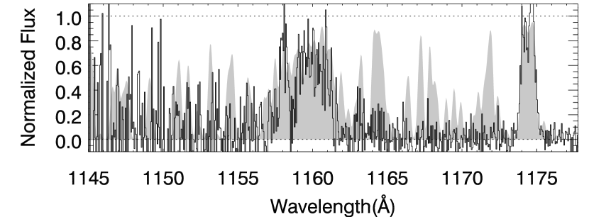
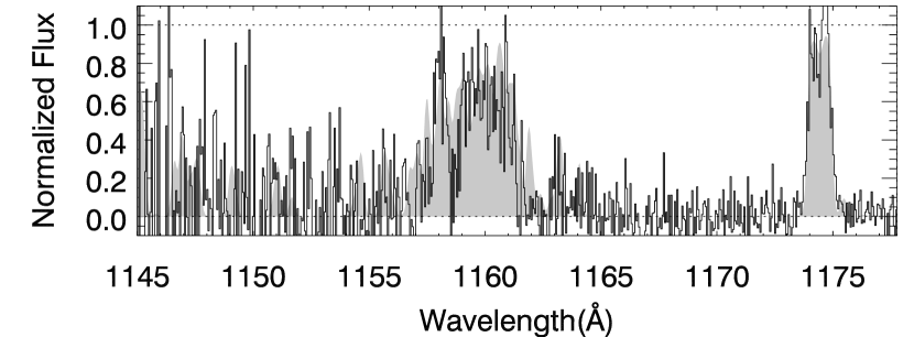
Figure 9: Comparison of models of the He II Gunn-Peterson trough (shaded) to observations (line). Assuming only 2 AGN close to the line of sight to HE 2347-4342, the opacity gaps are well reproduced but not the spectral ranges of high opacity (top panel). In addition to the 2 AGN, we have added 7 ‘soft’ sources close to the line of sight (bottom panel). The increased amount of H I ionizing photons lead to a larger $\Gamma_{\mathrm{HI}}$ and, therefore, to a larger softness parameter $S$.

Figure 9 presents the results for two different models. The top panel shows the calculated appearance of the He II Gunn-Peterson trough if only two AGN are present on the line of sight towards HE 2347-4342 (catalog ). Their characteristics are listed in the first two lines of Table 2 and model the opacity gaps as well as possible. Note that the 3rd and 4th columns give the luminosities for isotropic sources. The values are relatively well constrained (within 50%). The following two columns list the corresponding expected fluxes. They indicate that the sources responsible for the opacity gaps should be easily visible in the optical bands if they are not hidden by dust: the sources responsible for the $z=2.815$ and 2.866 gaps should have a magnitude $R\simeq 18.9$ and 20.2, respectively, if they have a flat spectrum in $f_{\lambda}$. A better approach to reveal them is to search for X-ray sources with Chandra or XMM-Newton. Compared to the simple model presented earlier (§5.2), the fact that we now take into account the presence of individual absorption lines allows us to reproduce the sharpness of the $z=2.866$ opacity gap. However, it is clear that such a model is unable to reproduce the high opacity regions, such as regions $C$, $D$ and $E$. The model shown in the bottom panel of Fig. 9 seems to reproduce the observed spectrum much better: its characteristics are discussed in the next section.

5.3.4 Possible origins for the high opacity regions

It is worth discussing the possible origins for the high opacity regions. In this section, we limit ourselves to two scenarios both compatible with photo-ionization, although not necessarily with photo-ionization equilibrium. In particular, these two models are compatible with the map of the softness parameter shown in Fig. 4. First, we recall the delayed re-ionization model invoked by Reimers et al. (1997). Then, we introduce a soft source model. Possible alternatives to these two models will be discussed later (§5.4).

The delayed re-ionization model (Reimers et al., 1997) suggests that the spectral ranges that show a large softness $S$ arise from regions of the Universe where hydrogen has been already mostly re-ionized but where the He II ion density $n_{\mathrm{HeII}}$ is still larger than in regions of mean $S$. The reduced He II ionizing photon flux causing the larger $n_{\mathrm{HeII}}$ results from the fact that He II ionizing photons has not yet managed to doubly ionize He in the intergalactic medium; in other words, the regions of large $\tau_{\mathrm{HeII}}$ are still shielded from the sources of He II ionizing photons due to the relatively large $n_{\mathrm{HeII}}$ in the intergalactic medium. In this model, the H I ionization rate $\Gamma_{\mathrm{HI}}$ is typically constant over the redshift range of interest, but the He II ionization rate $\Gamma_{\mathrm{HeII}}$ is small. An implicit hypothesis of this model is that the sources of both H I and He II ionizing photons are distant from the regions of large $\tau_{\mathrm{HeII}}$.

Here, we propose a second scenario: the presence of soft sources close to the line-of-sight of the quasar lead to a local increase of H I ionizing photons without providing additional He II ionizing photons. Such sources could be galaxies, e.g. Lyman-break galaxies which have recently been found to have a significant flux below 1 Ryd (Steidel, Pettini, & Adelberger, 2000). They can also be quasars similar to HE 2347-4342 (catalog ), i.e. which have $z_{\mathrm{abs}}\simeq z_{\mathrm{em}}$ absorption systems that are basically transparent to H I ionizing photons but opaque to He II ones. A third, although less likely, possibility is a normal quasar close to the line of sight but located behind a cloud with an H I column density low enough that the cloud is optically thin for H I ionizing photons (i.e., $\log{N_{\mathrm{HI}}}\lesssim 17$) but with an He II column density large enough to be optically thick to He II ionizing photons (i.e., $\log{N_{\mathrm{HeII}}}\gtrsim 18$). In this scenario, the intensity of the UV background at the He II Lyman limit is relatively similar in regions of mean or large $S$, as it is determined by (not too) distant sources, while the intensity at the H I Lyman limit is increased by a large factor due to the presence of the soft sources close to the line-of-sight.

The bottom panel of Fig. 9 illustrates how the introduction of a small number of soft sources can reproduce the observed spectrum of HE 2347-4342 (catalog ). The only constraints imposed on this model is that the mean opacities in each regions are broadly met and, in particular, that no peak of transmitted flux appear in regions of high opacity. The solution shown here is certainly not unique: we have no way to determine even the number of sources involved. In particular, such a lack of constraints means that we may as well choose a small number of bright sources as a large number of faint ones. In addition, since the lines composing the diffuse component are not observed but have their characteristics randomly selected, different realizations lead to slight differences in the appearance of the simulated He II Gunn-Peterson trough even for identical model parameters. For illustrative purposes, we list in Table 2 the parameters used for the solution shown in the Fig. 9 (bottom panel). The hard sources were discussed in the previous section. On the other hand, we see that the ‘soft’ sources should be revealed in deep images of the field. In the model described above, the sources are relatively bright galaxies and should be easily detectable ($R\sim 20.6$ to $21.4$). In this case, their local space density is $\sim 10^{-1}~{}(\mbox{comoving ~{} Mpc})^{-3}$, a factor $\sim 10^{3}$ larger than for Lyman break galaxies (LBG, Steidel et al., 1996). However, the important quantity is the number density of He II ionizing photons or luminosity density. Therefore, the sources can be more numerous and fainter and may indicate the presence of a proto-cluster close to the line of sight towards HE 2347-4342 (catalog ). The steepness of the luminosity function of the LBG (Steidel et al., 1999) actually insures that the required luminosity density can be obtained with a space density of galaxies comparable to the LBG one. Steidel, Pettini, & Adelberger (2000) showed that their contribution to the UV background intensity is important and can be predominant compared to the QSO one, but still be compatible with the value of the UV background intensity at the H I Lyman limit as measured by the proximity effect. It is also possible that most of the H I ionizing photons are produced by one AGN, as bright at 1 Rd as the one causing the $z=2.817$ opacity gap, but with a negligible flux of He II ionizing photons. Despite the uncertainty in the mix of ionizing sources, the important point is that photoionization alone allows us to reproduce the observations.

Figure 10 shows the map of the softness parameter corresponding to the model shown at the bottom panel of Fig. 9. Interestingly, the softness reaches values close to $S\sim 1\times 10^{4}$ at its peaks, where the line of sight is closer to the sources. If the impact parameters are even smaller than considered here, one can expect even larger value of $S$ as well as formation of absorption lines, such as C IV and Si IV. Therefore, the situation presented here is consistent with the large values of the Si IV to C IV column density ratios seen in quasar absorption lines which we examined in §4.3.

Of course, it may very well be that the two scenarios could co-exist even over a small redshift range. But can existing observations allow us to discriminate between the two models? We first note that in the delayed ionization model, the H I lines should have the same mean number density and column density distribution in spectral ranges of mean or large $S$ (i.e., opacity gaps excluded). However, in regions where He II re-ionization is delayed, the temperature of the gas is expected to be lower and therefore the Doppler $b$-parameter of the lines should be smaller than in regions where the He II re-ionization has taken place Schaye et al. (2000).

Since the line broadening is mostly turbulent, the best way to test this hypothesis would be to compare the cut-off $b_{\mathrm{c}}$ seen in the $b$ distribution (e.g., Kim, Hu, Cowie & Songaila, 1997) of the H I lines: we would expect $b_{\mathrm{c}}$ to be smaller for the lines whose corresponding He II lines fall in the regions $C$ and $D$ than for the rest of the spectrum. However, a reliable determination of $b_{\mathrm{c}}$ requires a large number of lines in the sample, $\sim 200$ (Schaye, Theuns, Leonard & Efstathiou, 1999), while only 15 are detected in regions $C$ and $D$. Therefore, we can only compare the mean $\bar{b}$ and standard deviation $\sigma(b)$ of the $b$ parameters for the two samples. We find them to be similar, with $\bar{b}_{\mathrm{C,D}}=32\pm 13~{}\mbox{km}~{}\mbox{s}^{-1}$ compared to $\bar{b}_{\mathrm{other}}=34\pm 17~{}\mbox{km}~{}\mbox{s}^{-1}$. In addition, a 2-sided Kolmogorov-Smirnov test of the samples of $b$ values gives a D statistic of 0.22 with a probability of 0.53 that it arises by chance. In other words, the two samples appear drawn from the same population. Unfortunately, the small number of lines used for the test makes it of limited use.

On the other hand, in the soft sources model, one expects an increase of the H I ionization fraction of the gas and therefore a local decrease in the number density and column density of the H I lines. Comparison between the number of lines observed in regions $C$ and $D$ and the number of lines expected based on the observations by Kim, Hu, Cowie & Songaila (1997) show agreements for different column density cut-off. We note, however, that the scatter in the number of expected lines is itself much larger than if the error were purely Poissonian so that this test is not very sensitive over a small spectral range. However, it is worth noting that the region of low H I opacity at $z\sim 2.855$ is quite remarkable for its extent: we measure $\tau_{\mathrm{HI}}\simeq 0.0085$ over a spectral range larger than $\Delta\lambda=6.5$Å  (of course, such a measure is largely affected by errors on the continuum definition). There is no occurrence of such a large spectral range with such low H I opacity in the spectrum of HE 2347-4342 (catalog ) before $z=2.6$. Another way to express this observation is that there is no line with $N_{\mathrm{HI}}>3\times 10^{12}~{}\mathrm{cm}^{-2}$ over this spectral range. From Table 4 of Kim, Hu, Cowie & Songaila (1997), the H I column density distribution at a mean redshift $\bar{z}=2.85$ is $f(N_{\mathrm{HI}})=4.9\times 10^{7}~{}N_{\mathrm{HI}}^{-1.46}$. Therefore, we expect to see $\sim 760$ lines with $N_{\mathrm{HI}}>3\times 10^{12}~{}\mathrm{cm}^{-2}$ per unit redshift, or about 4 such lines over a spectral range of 6.5Å  at $z\simeq 2.885$. For a Poisson distribution, the a posteriori probability that no such lines are seen is $<0.02$. An additional argument in favor of the soft sources model come from the recent study by Boksenberg, Sargent, & Rauch (2001): by comparing the Si IV/C IV vs the C II/C IV ratio over the range $1.9<z<4.4$ with CLOUDY models, they find that the data are best explained by a UV background dominated by QSOs at low redshift but that a dominating stellar contribution is progressively required at higher redshift.

Finally, we should note that in the absence of soft sources, within the delayed reionization model, the high opacity in regions $A$, $C$ and $D$ puts constraints either on the the lifetime or the luminosity of the AGN causing the opacity gaps. Indeed, let us suppose that the opacity gap at $z=2.86$ is indeed caused by an AGN whose characteristics are close to the values given in Table 2. Therefore, the large opacity in regions $A$, $C$ and $D$ indicates at least one of the two following conclusions:

(i) Let us assume that there are no high column density systems (including systems intrinsic to the AGN) on the light path between the AGN (located off the line-of-sight) and regions $A$ to $D$ and that the time that was required to photo-ionize the region $B$, $t_{\mathrm{phot}}$, is similar to the time required to photo-ionize the regions $A$, $C$ and $D$. Therefore, the difference between the lifetime of the AGN, $t_{\mathrm{AGN}}$, and $t_{\mathrm{phot}}$ is larger than the time required for light to go from the AGN to region $B$ but smaller than the time required to go from the AGN to any of the regions $A$, $C$ and, a fortiori, $D$. Consequently, we have $10^{6}~{}\mathrm{yr}\lesssim t_{\mathrm{AGN}}-t_{\mathrm{phot}}\lesssim 10\times 10^{6}~{}\mathrm{yr}$, compatible with currently admitted AGN lifetime.

(ii) In unification scheme models, the AGN continuum region may be surrounded by a molecular torus optically thick to both H I and He II ionizing photons. In this case, the model that we have developed would require to take into account more variables. Indeed, the size and shape of the opacity gaps will not only be determined by the luminosities and impact parameters of the responsible AGN but also by the orientation of the ionizing radiation cone relative to the line of sight towards HE 2347-4342 (catalog ). Of course, the possible configurations are numerous. However, it is interesting to consider the possibility that the ionizing cones are oriented perpendicularly to the line of sight towards HE 2347-4342 (catalog ) as this configuration allows to derive lower limits to the AGN luminosities. In the case of the $z=2.866$ opacity gap, region $B$ alone would see the continuum region while the torus blocks ionizing photons to reach regions $A$, $C$ and $D$, and therefore would explain their high He II opacity in the absence of other hard sources. Since region $B$ extends over $\sim 3$ comoving Mpc, and assuming a half-opening angle of $\sim 45$ deg (Barthel, 1989), we derive an impact parameter of $\sim 1.5$ comoving Mpc for the AGN. Since this value is only slightly larger (50%) than the impact parameter we found above (cf. Table 2), the luminosity of the AGN should be at least of the same order of magnitude as listed in Table 2. We can do the same exercise for the $z=2.817$ opacity gap. The comoving distance between its extremities (broadly taken to be from 1157.75Å  to 1162Å, although residual signals are detected at the 3$\sigma$ levels in regions $E$ and $H$) is $\sim 15$ comoving Mpc. Therefore, the impact parameter would be $\sim 7.5$ comoving Mpc, also about 50% larger than the value listed in Table 2. Consequently, we find that for two models of AGN (with and without optically thick molecular torus), Table 2 lists at least lower limits to their luminosities.

In summary, there is no clear explanation for the high opacity seen in the spectrum of HE 2347-4342 (catalog ), especially in regions $C$ and $D$. Tests based on the width of the H I lines are inconclusive mainly because of the small number of lines available. Within the delayed reionization model, we can provide some constraints on the lifetime, compatible with currently admitted values, or lower limits to the luminosity of the AGN causing the opacity gaps. However, the large region of low H I opacity is more easily explained in the soft sources model. Consequently, a search for $z\sim 2.8$ Lyman Break galaxies in this field would be interesting in order to test the soft sources model, while a search for AGN with Chandra or XMM-Newton could indicate the presence of a molecular torus.

5.4 Alternative explanations?

In the previous sections, we only considered photoionization as the main process responsible for the different features seen in the spectra of HE 2347-4342 (catalog ). In Heap et al. (2000), we also examined two alternative explanations to the opacity gaps, as arising in low-density regions or caused by shock-heated gas, and we will not consider them any further. We only note that the 5 H I lines that appear within the opacity gaps have a $\bar{b}_{\mathrm{gaps}}=30\pm 8~{}\mbox{km}~{}\mbox{s}^{-1}$, which is consistent with the values derived in other parts of the spectrum (cf. above). In other words, the temperature within the opacity gaps does not seem to be significantly different from regions of high opacity. Instead, we can wonder if photoionization is the only explanation for the high opacity seen in the spectral ranges $C$ and $D$ where few H I lines are seen. Clearly, such regions are not affected by low gas density, since it would be difficult to explain the large He II opacity. Can collisions ionize the H I without ionizing He II? If this was the case, we would expect that the gas be warmer in regions where collisional ionization is the most important process. Therefore, we would expect that the Doppler $b$ parameter of the H I lines in these regions to be significantly larger than elsewhere. In the previous section, we already compared the $b$ parameter of the lines in regions $C$ and $D$ to the ones in other regions and found no significant difference in the median value of the two samples. Within the limits of validity of this test, mainly due to the small sample of lines, we conclude that there is no indication that collisional ionization is responsible for the small H I line number density in regions $C$ and $D$.

Finally, it could also be that part of the observed opacity in region $C$ and $D$ is actually due partially to metal absorption lines associated either with the Milky Way or with intervening systems. However, existing spectra at longer wavelengths do not reveal any strong systems at the appropriate redshifts. Similarly, we do not expect any strong Galactic lines at $\lambda\sim 1170$Å.

6 Conclusions

6.1 Observational results

In this paper, we have presented HST STIS spectra of HE 2347-4342 (catalog ). The brightness of the quasar permits the use of the G140M grating which provides a much improved resolution (0.16 Å) compared to the data obtained by Reimers et al. (1997) (0.7 Å) with the GHRS. The 2 dimensional nature of the FUV MAMA detector allowed us to better quantify the background due to the sky and (mainly) the dark current. We confirm the findings by Reimers et al. (1997) that the spectrum presents regions of high opacity, some of them devoid of corresponding H I lines, and regions of low opacities (opacity gaps) that match regions displaying a low number density of H I lines.

We improve significantly the lower limits on the Gunn-Peterson opacity in the high opacity regions. In particular, we find $\tau_{\mathrm{HeII}}=4.80_{-0.80}^{+\infty}$ in region $C$. Even at the lowest redshift recorded by the STIS spectrum, the opacity is still $\tau_{\mathrm{HeII}}=2.57_{-0.41}^{+0.72}$. This value is significantly larger than the value of 1.9 measured by Heap et al. (2000) in the spectral range $S$ of the spectrum of Q 0302-003 (catalog ) with a redshift range comparable to the STIS spectrum of HE 2347-4342 (catalog ).

Another interesting feature is the absence of the proximity effect already noticed by Reimers et al. (1997). It is easy to show that the large He II column density required to account for the large opacity in the spectral region affected by the $z_{\mathrm{abs}}\simeq z_{\mathrm{em}}$ absorption also implies that the amount of He II ionizing photons escaping is reduced to a very small quantity. It is interesting to speculate on the effects of such systems on the UV background radiation. Of the 4 objects for which the He II Gunn-Peterson absorption has been observed, only two show the proximity effect (Q 0302-003 (catalog ) and PKS 1935-692 (catalog )). The other two (HS 1700+6416 (catalog ) and HE 2347-4342 (catalog )) also show strong $z_{\mathrm{abs}}\simeq z_{\mathrm{em}}$ systems, with evidence of line locking (cf. Tripp, Lu, & Savage, 1997, for HS 1700+6416 and Smette & Songaila, in preparation, for HE 2347-4342), which indicates that the absorption takes place close to the quasar continuum emitting region. If these 4 quasars are representative of the quasar population as a whole – which is probably not the case, as Foltz et al. (1986) and Møller & Jakobsen (1987)) find a dependence of the number of $z_{\mathrm{abs}}\simeq z_{\mathrm{em}}$ systems in quasar samples either on their radio-loudness or both their radio-loudness and optical luminosity – then one can expect that only half of the He II ionizing photons escape from the known quasar population relative to the case where all quasars emit He II ionizing photons. Consequently, we would expect that the He II photoionization rate be reduced by a significant factor in models where the UV background radiation is dominated by quasars, leading naturally to a softer UV background. Another expected consequence of the fact that only a fraction of the QSOs actually provide He II ionizing photons is that the UV background He II photoionization rate should show stronger fluctuations than predicted by current models (e.g. Fardal et al., 1998), since even fewer quasars would contribute to the He II ionizing flux at a given point.

6.2 Modeling

Comparison between the H I and the He II spectra allowed us to build a one-dimensional map of the softness of the UV background radiation. Except in the opacity gaps, the observed UV background is significantly softer than model predictions assuming a QSO-dominated UV background (e.g. Haardt & Madau, 1996; Fardal et al., 1998; Madau et al., 1999). In spectral ranges $C$ and $D$, it is even larger than the one predicted for a UV background whose intensity at 1 Rd has equal contributions from stars and AGN (cf. Fardal et al., 1998, for some examples). Large values of the softness parameters are in agreement with the large observed Si IV to C IV ratios seen in quasar absorption line systems.

We have presented a simple model to describe the opacity gaps caused by photoionization due to ‘hard’ sources located close to the line of sight to the background quasar. Away from individual absorption lines, it indicates that the extent of the gap is related to the source luminosity, while, for a given extent, the amount of transmitted flux at the center of the gap is directly related to the distance of the source to the line of sight. Finally, we have expanded the model of the He II Gunn-Peterson trough presented in Heap et al. (2000) to account for multiple sources close to the line of sight. It allows us to make relatively precise predictions concerning the intrinsic luminosity of the sources causing the opacity gaps, which should be easily detectable with Chandra or XMM-Newton.

We discussed the possible origin of the regions of high He II opacity but low H I opacity. We introduce a new model where they are caused by nearby soft sources. If only a small number of these sources are present close to the line of sight, they should be bright and easily observable. However, we have few constraints on their number so that they could be much fainter and more numerous, with a space density comparable with the Lyman Break galaxies. We compare this model with the delayed re-ioniation scenario proposed by Reimers et al. (1997). There is no clear argument which leads us to favor of one or the other model to explain the high He II opacity in these regions. Within the delayed re-ionization model, if opacity gaps are indeed caused by AGN, the presence of a high opacity region close to an opacity gap provide reasonable constraints on the lifetime or luminosities of the AGN. On the other hand, soft sources would more easily explain the large region of low H I opacity seen at the same redshift as region $C$. Optical search for Lyman break galaxies and X-ray observations can probably settle the issue.

While this paper was being revised, Kriss et al. (2001) presented FUSE observations of the line of sight towards HE 2347-4342 (catalog ), covering a much longer redshift range ($2.3<z<2.7$) and twice higher resolution ($R\sim 15,000$) than our HST STIS observations. However, over the common wavelength range, our data show a larger signal-to-noise ratio and especially better controlled systematic errors (mainly due to the better background determination made possible by the the STIS FUV-MAMA detector compared to the FUSE ones), that allow us to provide better contraints on the He II Gunn-Peterson optical depth. The behavior seen in the HST GHRS and STIS observations, i.e., alternance of regions of low and high opacity is confirmed and seen over the whole spectral range covered by the FUSE observations. In the FUSE spectrum, the optical depths measured over spectral ranges of $\sim 5$Å  appear to converge towards theoretically predicted values (e.g. Fardal et al., 1998; Machacek et al., 2000) at $z<2.75$ but are systematically larger than predictions in the redshift range common to both FUSE and STIS observations. Comparison between the FUSE observations and the corresponding Keck–HIRES H I spectrum shows that $\eta\equiv N_{\mathrm{HeII}}/N_{\mathrm{HI}}$ varies between $\sim 1$ to at least several hundreds, as in the STIS spectral range. In accord with the findings of this paper, Kriss et al. (2001) conclude that these regions of large $\eta$ (or softness parameter $S\propto\eta$) are subject to a much softer background radiation either because of delayed He II re-ionization or due to the presence of ‘soft’ sources close to the line-of-sight. Although both explanations are equally possible over some spectral range, the fact that excursions of $\eta$ towards large values continue to $z\sim 2.3$ probably favour the latter one.

Figure 1: Spectra of HE 2347–4342 (catalog ). (Top:) Keck–HIRES spectrum. The original spectrum has been normalized by a spline function passing through spectral ranges apparently devoid of absorption lines. Wavelengths have been multiplied by the ratio of the wavelengths of He II to H I Ly-$\alpha$ lines $\lambda_{\mathrm{HeII}}/\lambda_{\mathrm{HI}}=303.7822/1215.6701$. (Bottom:) HST STIS FUV MAMA G140M spectrum. The original spectrum has been normalized assuming that the underlying quasar continuum has an observed flux constant with wavelength of $f_{\lambda}=2.53~{}\times~{}10^{-15}~{}\mbox{ergs}~{}\mbox{s}^{-1}~{}\mbox{cm}^{-2}~{}\mbox{\AA}^{-1}$. The thin dotted line represents the 1-$\sigma$ error array. No sign of He II Ly-$\alpha$ emission line is present; its center is expected to fall at $\lambda=1180$, indicated by the thick vertical dotted line. In both panels, the vertical dashed line at $\sim 1178~{}\mbox{\AA}$ corresponds to $z=2.877$, redwards of which the spectra are likely to be affected by the known $z_{\mathrm{abs}}\simeq z_{\mathrm{em}}$ systems (Reimers et al., 1997). Wavelengths are vacuum heliocentric.

Figure 2: Normalized STIS spectrum of HE 2347–4342. We have also represented by a rectangle the mean and uncertainty of the transmitted flux for each of the spectral ranges defined in Table 1. For each rectangle, the width represents the wavelength range of the corresponding region, the central line represents its mean transmitted flux and its thickness is equal to twice the measurement uncertainty.

Figure 3: Measurements of the He II Gunn-Peterson opacity at $z>2.75$. The value measured by Davidsen, Kriss, & Zheng (1996) towards HS 1700+6416 (catalog ) is $\tau_{\mathrm{HeII}}=1.0\pm 0.07$ over the range $2.2<z<2.6$. For comparison, the dashed and dotted lines show the optical depths predicted by two models considered by Machacek et al. (2000) that bracket the range of models in their study.

Figure 4: Softness parameter for different spectral ranges in the spectrum of HE 2347–4342 (catalog ). The width of each symbol covers the redshift range of the corresponding region. Arrows represent 3 $\sigma$ lower limits, i.e., they correspond to spectral ranges over which the mean normalized flux $\bar{I}<3~{}\sigma_{\mathrm{I}}$. The dashed line represents the softness parameter of the model calculated by Madau et al. (1999) at $z=2.76$. The dotted line gives the softness parameter of one of the models calculated by Fardal et al. (1998), for which the stellar contribution is fixed at 912 Å  to have an emissivity twice that of the quasars (cf. text).

Figure 5: Comparison of the Si IV/C IV versus C II/C IV column density ratios observed in QSO absorption line systems at $z_{\rm abs}>$ 3.00 (filled circles) and $z_{\rm abs}<$ 3.00 (open circles) from Songaila (1998) to the ratios predicted by photoionization models for three different radiation fields. The radiation fields assumed for the three models have softness parameters $S=\Gamma_{\rm H~{}I}/\Gamma_{\rm He~{}II}$ ranging from $S$ = 130 to $S$ = 9530. The ratios predicted by a photoionization model which assumes the UV background at $z$ = 3 due to QSOs only from the calculation of Fardal et al. (1998) is shown with a solid line; this radiation field has $S$ = 130. The photoionization models shown with dashed and dotted lines assume the same QSO background plus a hot star (see text) which is 10 or 50 times brighter than the QSO background at the H I Lyman limit. These models have $S$ = 2010 and 9530, respectively.

Figure 6: Simple model for the opacity gaps. Left panels: Schematic plan view of the different examples discussed in the text. The stars represent the ‘hard’ sources S1 or S2, of luminosities $L^{\mathrm{S1}}=2.5\times 10^{29}~{}\mbox{ergs}~{}\mbox{s}^{-1}~{}\mbox{Hz}^{-1}$ (panel (A) and (B)) and $L^{\mathrm{S2}}=L^{\mathrm{S1}}/10$ (panel (C)). The solid circles indicate where the photoionization rate due to the source S$i$ $\Gamma_{\mathrm{HeII}}^{\mathrm{S}i}$ equals the one due to the UV background assumed to be $\Gamma_{\mathrm{HeII}}^{\mathrm{J}}=3.75\times 10^{-15}~{}\mbox{ergs}~{}\mbox{s}^{-1}~{}\mbox{Hz}^{-1}~{}\mbox{sr}^{-1}$. The dotted lines represent the lines of sight passing close to the source S$i$. Right panels: Corresponding shapes for the opacity gaps. The dashed lines indicate where $\Gamma_{\mathrm{HeII}}^{\mathrm{S}i}=\Gamma_{\mathrm{HeII}}^{\mathrm{J}}$, leading to $\tau_{\mathrm{HeII}}=\tau_{\mathrm{max}}/2$ (i.e., $\tau_{\mathrm{HeII}}=2.25$ in these examples).

Figure 7: Models for the observed opacity gaps. Left panel: Model for the $z=2.817$ gap. Right panel: Best attempt to model the $z=2.866$ gap. Such a simple model of course fails to reproduce the effect of individual absorption lines which probably causes the sharpness of the profile.

Figure 8: Schematic representation of the distribution of clouds (thin lines) and sources between the observer ($O$) and the background quasar ($Q$). ‘Hard’ and ‘soft’ sources are represented by filled and open stars, respectively. The regions where the H I and He II photoionization rates due to each source equal the UV background ones are represented by the solid and dashed circles, respectively.

Figure 10: Softness parameter as a function of redshift for the model considered in Fig. 9, bottom panel.

Table 1: Measured He II opacities

Spectral range	Wavelength	Mean	Mean	$\tau_{\mathrm{HeII}}$
	range	redshift	normalized
	(Å)		flux
A	1175.60–1178.00	2.8738	$\phantom{-}0.018\pm 0.009$	$4.00^{+0.67}_{-0.40}$
B	1174.00–1174.90	2.8661	$\phantom{-}0.930\pm 0.040$	$0.07^{+0.04}_{-0.04}$
C	1170.00–1173.50	2.8572	$\phantom{-}0.008\pm 0.010$	$4.80^{+\infty}_{-0.80}$
D	1165.00–1169.95	2.8431	$-0.009\pm 0.011$	$>4.54$
E	1162.00–1165.00	2.8300	$\phantom{-}0.057\pm 0.018$	$2.86^{+0.39}_{-0.28}$
F	1159.00–1161.00	2.8185	$\phantom{-}0.642\pm 0.038$	$0.44^{+0.06}_{-0.06}$
G	1157.75–1158.25	2.8119	$\phantom{-}0.783\pm 0.090$	$0.24^{+0.12}_{-0.11}$
H	1155.00–1157.75	2.8066	$\phantom{-}0.096\pm 0.032$	$2.34^{+0.40}_{-0.28}$
I	1150.00–1154.95	2.7938	$\phantom{-}0.024\pm 0.030$	$3.72^{+\infty}_{-0.81}$
J	1145.00–1149.95	2.7773	$\phantom{-}0.076\pm 0.039$	$2.57^{+0.72}_{-0.41}$
C+D	1165.00–1173.50	2.8490	$-0.001\pm 0.007$	$>4.90$
I+J	1145.00–1154.95	2.7856	$\phantom{-}0.049\pm 0.025$	$3.02^{+0.70}_{-0.41}$

Table 2: Model parameters

Source	$z_{s}$	$L_{\mathrm{HI}}^{s}$	$L_{\mathrm{HeII}}^{s}$	$f_{\mathrm{HI}}^{s}$	$f_{\mathrm{HeII}}^{s}$	$p^{s}$	Comments
	2.885	$220$	.	250	.	0	HE 2347-4342
1	2.81500	$4.1$	$0.25$	5.0	5.0	4.2	hard source (AGN)
2	2.86609	$1.3$	$0.08$	1.5	1.5	1.0	hard source (AGN)
3	2.79583	$0.4$	.	0.5	.	0.8	soft source
4	2.83000	$0.4$	.	0.5	.	0.4	soft source
5	2.83200	$0.4$	.	0.5	.	0.4	soft source
6	2.84100	$0.4$	.	0.5	.	0.4	soft source
7	2.84300	$0.4$	.	0.5	.	0.4	soft source
8	2.85000	$0.4$	.	0.5	.	0.4	soft source
9	2.85800	$0.8$	.	1.0	.	0.4	soft source

References

- Anderson et al. (1999) Anderson, S. F., Hogan, C. J., Williams, B. F., & Carswell, R. F. 1999, AJ, 117, 56
- Barthel (1989) Barthel, P. D. 1989, ApJ, 336, 606
- Bevington & Robinson (1992) Bevington, P.R., & Robinson, D.K. 1992, Data Reduction and Error Analysis for the Physical Sciences (2d ed.; New York : McGraw-Hill)
- Boksenberg, Sargent, & Rauch (2001) Boksenberg, A., Sargent, W.L.W., & Rauch 2001, submitted to ApJS
- Brown et al. (2000) Brown, T.M., Kimble, R.A., Ferguson, H.C., Gardner, J.P., Collins, N.R. & Hill, R. S. 2000, AJ, 120, 1153
- Croft et al. (1997) Croft, R. A. C., Weinberg, D. H., Katz, N., & Hernquist, L. 1997, ApJ, 488, 532
- Davidsen, Kriss, & Zheng (1996) Davidsen, A.F., Kriss, G.A., & Zheng, W., 1996, Nature, 380, 47
- Fardal et al. (1998) Fardal, M.A., Giroux, M.L., & Shull, J.M. 1998, AJ, 115, 2206
- Ferland et al. (1998) Ferland, G. J., Korista, K. T., Verner, D. A., Ferguson, J. W., Kingdon, J. B., & Verner, E. M. 1998, PASP, 110, 761
- Foltz et al. (1986) Foltz, C. B., Weymann, R.J., Peterson, B.M., Sun, L., Malkan, M.A. & Chaffee, F.H. 1986, ApJ, 307, 504
- Fontana & Ballester (1995) Fontana, A., & Ballester, P. 1995, ESO Messenger, 80, 37
- Giroux & Shull (1997) Giroux, M. L., & Shull, J. M. 1997, AJ, 113, 1505
- Gunn & Peterson (1965) Gunn, J., & Peterson, B. 1965, ApJ, 142, 1633
- Jakobsen et al. (1994) Jakobsen, P. , Boksenberg, A., Deharveng, J.M., Greenfield, P., Jedrzejewski, R., Paresce, F. 1994, Nature, 370, 35
- Haardt & Madau (1996) Haardt, F., & Madau, P. 1996, ApJ, 461, 20
- Heap et al. (2000) Heap, S.R., Williger, G.M., Smette, A., Hubeny, I., Sahu, M.S., Jenkins, E.B., Tripp, T.M., Winkler, J.N. 2000, ApJ, 534, 69
- Hogan, Anderson & Rugers (1997) Hogan, C.J., Anderson, S.F. & Rugers, M.H. 1997, AJ, 113, 1495
- Kayser, Helbig & Schramm (1997) Kayser, R., Helbig, P. & Schramm, T. 1997, A&A, 318, 680
- Kepner et al. (1999) Kepner, J., Tripp, T. M., Abel, T., & Spergel, D. 1999, AJ, 117, 2063
- Kim, Cristiani & D’Odorico (2001) Kim, Tae-Sun, Cristiani, S., & D’Odorico, S. 2001, A&A, submitted
- Kim, Hu, Cowie & Songaila (1997) Kim, T., Hu, E.M., Cowie, L.L. & Songaila, A. 1997, AJ, 114, 1
- Kimble et al. (1998) Kimble, R.A. et al. 1998, ApJ, 492, L83
- Kriss et al. (2001) Kriss, G. A. et al. 2001, Science, 293, 1112
- Kurucz (1991) Kurucz, R. L. 1991, in Proceedings of the Workshop on Precision Photometry: Astrophysics of the Galaxy, ed. A. C. Davis Philip, A. R. Upgren, & K. A. James (Davis, Schenectady), p27
- Leitherer et al. (2000) Leitherer, C., et al. 2000, STIS Instrument Handbook , Version 4.1, (Baltimore: STScI)
- Lindler (1998) Lindler, D.J. 1998, CALSTIS Reference Guide (Version 5.1), http://hires.gsfc.nasa.gov/stis/software/software.html
- Machacek et al. (2000) Machacek, M.E., Bryan, G.L., Meiksin, A., Anninos, P., Thayer, D., Norman, M., & Zhang, Y. 2000, ApJ, 532, 118
- Madau et al. (1999) Madau, P., Haardt, F., & Rees, M. J. 1999, ApJ, 514, 648
- McWilliam (1997) McWilliam, A. 1997, ARA&A, 35, 503
- Miralda-Escudé, Haehnelt, & Rees (2000) Miralda-Escudé, J., Haehnelt, M., & Rees, M.J. 2000, ApJ, 530, 1
- Møller & Jakobsen (1987) Møller, P. & Jakobsen, P. 1987, ApJ, 320, L75
- Møller & Jakobsen (1990) Møller, P. & Jakobsen, P. 1990, A&A, 228, 299
- Osterbrock (1989) Osterbrock, D.E. 1989, Astrophysics of Gaseous Nebulae and Active Galactic Nuclei. Mill Valley, Calif. University Science Books, 1989
- Picard & Jakobsen (1993) Picard, A., & Jakobsen, P. 1993, A&A, 276, 331
- Pei (1992) Pei, Y.C., 1992, ApJ, 395, 130
- Rauch (1998) Rauch, M. 1998, ARA&A, 36, 267
- Reimers et al. (1997) Reimers, D., Köhler, S., Wisotzki, L., Groote, D., Rodriguez-Pascual, P., & Wamsteker, W. 1997, A&A, 327, 890
- Robertson (1986) Robertson, J. G. 1986, PASP, 98, 1220
- Savaglio et al. (1997) Savaglio, S., Cristiani, S., D’Odorico, S., Fontana, A., Giallongo, E., & Molaro, P. 1997, A&A, 318, 347
- Schaye, Theuns, Leonard & Efstathiou (1999) Schaye, J., Theuns, T., Leonard, A. & Efstathiou, G. 1999, MNRAS, 310, 57
- Schaye et al. (2000) Schaye, J., Theuns, T., Rauch, M., Efstathiou, G., & Sargent, W. L. W. 2000, MNRAS, 318, 817
- Scheuer (1965) Scheuer, P. 1965, Nature, 207, 963
- Schlegel et al. (1998) Schlegel, D.J., Finkbeiner, D.P. Davis, M. 1998, ApJ, 500, 525
- Stark et al. (1992) Stark, A.A., Gammie, C.F., Wilson, R.W., Bally, J., Linke, R.A., Heiles, C. & Hurwitz, M. 1992, ApJS, 79, 77
- Steidel et al. (1996) Steidel, C.C., Giavalisco, M., Pettini, M., Dickinson, M., & Adelberger, K.L. 1996, ApJ, 462, L17
- Steidel et al. (1999) Steidel, C. C., Adelberger, K. L., Giavalisco, M., Dickinson, M., & Pettini, M. 1999, ApJ, 519, 1
- Steidel, Pettini, & Adelberger (2000) Steidel, C.C., Pettini, M., & Adelberger, K.L., ApJ, accepted, (astro-ph/0008283)
- Steidel, Pettini, & Adelberger (2001) Steidel, C. C., Pettini, M., & Adelberger, K. L. 2001, ApJ, 546, 665
- Songaila, Hu & Cowie (1995) Songaila, A., Hu, E.M. & Cowie, L.L. 1995, Nature, 375, 124
- Songaila & Cowie (1996) Songaila, A., Cowie, L.L., AJ112, 335
- Songaila (1998) Songaila, A. 1998, AJ, 115, 2184
- Timmes, Woosley, & Weaver (1995) Timmes, F. X., Woosley, S. E., & Weaver, T. A. 1995, ApJS, 98, 617
- Tripp, Lu, & Savage (1997) Tripp, T.M., Lu, L., & Savage, B.D. 1997, ApJS, 112, 1
- Tytler et al. (2000) Tytler, D., O’Meara, J.M., Suzuki, N. & Lubin, D. 2000, Physica Scripta Volume T, 85, 12
- Weymann, Carswell & Smith (1981) Weymann, R.J., Carswell, R.F. & Smith, M.G. 1981, ARA&A, 19, 41
- Woodgate et al. (1998) Woodgate, B.E. et al. 1998, PASP, 110, 1183
- Zheng & Davidsen (1995) Zheng, W., & Davidsen, A. 1995, ApJ, 440, L53