Confirmation of the existence of coherent orientations of quasar polarization vectors on cosmological scales

In order to verify the existence of coherent orientations of quasars polarization vectors on very large scales, we have obtained new polarization measurements for a sample of quasars located in a given region of the three-dimensional Universe where the range of polarization position angles was predicted in advance. For this new sample, the hypothesis of uniform distribution of polarization position angles may be rejected at the 1.8% significance level on the basis of a simple binomial test. This result provides an independent confirmation of the existence of alignments of quasar polarization vectors on very large scales. In total, out of 29 polarized quasars located in this region of the sky, 25 have their polarization vectors coherently oriented. This alignment occurs at redshifts $z\simeq$ 1-2 suggesting the presence of correlations in objects or fields on Gpc scales. More global statistical tests applied to the whole sample of polarized quasars distributed all over the sky confirm that polarization vectors are coherently oriented in a few groups of 20-30 quasars. Some constraints on the phenomenon are also derived. Considering more particularly the quasars in the selected region of the sky, we found that their polarization vectors are roughly parallel to the plane of the Local Supercluster. But the polarization vectors of objects along the same line of sight at lower redshifts are not accordingly aligned. We also found that the known correlations between quasar intrinsic properties and polarization are not destroyed by the alignment effect. Several possible mechanisms are discussed, but the interpretation of this orientation effect remains puzzling.

1 Introduction

Considering a sample of 170 optically polarized quasars with accurate polarization measurements, we recently found that quasar polarization vectors are not randomly oriented on the sky as naturally expected. Indeed, in some regions of the three-dimensional Universe (i.e. in regions delimited in right ascension, declination, and redshift), the quasar polarization position angles appear concentrated around preferential directions, suggesting the existence of large-scale coherent orientations –or alignments– of quasar polarization vectors (Hutsemékers 1998, hereafter Paper I).

Mainly because the polarization vectors of objects located along the same line of sight but at different redshifts are not accordingly aligned, possible instrumental bias and contamination by interstellar polarization are unlikely to be responsible for the observed effect (cf. Paper I for a more detailed discussion). The very large scale at which these coherent orientations are seen suggests the presence of correlations in objects or fields on spatial scales $\sim 1000\,h^{-1}$ Mpc at redshifts $z\simeq$ 1–2, possibly unveiling a new effect of cosmological importance.

Although we found this orientation effect statistically significant, the sample is not very large, and further investigation is needed to confirm it, especially in view of its very unexpected nature. One of the simplest tests consists in measuring the polarization of a new sample of quasars located in one of the regions of the sky where an alignment was previously found and where we can predict in advance the range of polarization position angles. Such polarimetric observations have been recently carried out, and the results are presented here.

In Sect. 2, we present the new polarimetric observations, as well as a compilation of the most recent measurements from the literature. The results of the statistical analysis –confirming the orientation effect– are given in Sect. 3. Then, from the properties of the objects in the region of alignment we derive some constraints on possible interpretations. These are discussed in Sect. 4. Conclusions form the last section.

2 New observations and compilation of data

In Paper I, we identified a region in the sky (region A1) where nearly all quasar polarization position angles lie in the range 146$\degr$ – 46$\degr$. This region is delimited in right ascension by $11^{h}15^{m}\leq\alpha\leq 14^{h}29^{m}$ and in redshift by $1.0\leq z\leq 2.3$.

A new sample of quasars located in this region was therefore selected, mainly from the quasar catalogues of Véron-Cetty & Véron (1998) and Hewitt & Burbidge (1993). This sample was observed during two runs at ESO La Silla in 1998 and 1999, using the ESO 3.6m telescope equipped with EFOSC2 in its polarimetric mode. In order to minimize the contamination by interstellar polarization in our Galaxy, only objects at high galactic latitudes $|b_{\scriptscriptstyle\rm II}|\geq 35\degr$ were considered. The selection of the targets at the telescope was not random: the brightest objects were given higher priority as well as objects at the center of the alignment region where the orientation effect is suspected to be stronger. Also, radio-loud and broad absorption line (BAL) quasars were preferred since these objects are more likely to be significantly polarized (Impey & Tapia 1990, Hutsemékers et al. 1998, Schmidt and Hines 1999). In this view, 3 BAL quasars recently discovered by Brotherthon et al. (1998) were added to the sample. At the end, polarimetric data were secured for 28 quasars belonging to region A1, with a typical uncertainty of 0.2% on the polarization degree. About half of them appear significantly polarized. These data are presented in Lamy & Hutsemékers (2000) with full account of the observation and reduction details.

Table 1: The additional sample of polarized quasars

Object	$b_{\scriptscriptstyle\rm II}$	$z$	$p$	$\sigma_{p}$	$\theta$	$\sigma_{\theta}$	Ref
(B1950)	($\degr$)		(%)	(%)	($\degr$)	($\degr$)
B0004$+$017	$-$59	1.711	1.29	0.28	122	6	8
B0010$-$002	$-$61	2.145	1.70	0.77	116	13	8
B0025$-$018	$-$64	2.076	1.16	0.52	109	13	8
B0046$-$315	$-$86	2.721	13.30	2.00	159	4	7
B0109$-$014	$-$64	1.758	1.77	0.35	76	6	8
B0117$-$180	$-$79	1.790	1.40	0.46	13	10	8
B0226$-$104	$-$62	2.256	2.51	0.25	165	3	8
B0422$-$380	$-$45	0.782	6.20	3.00	173	14	7
B0448$-$392	$-$40	1.288	2.90	1.00	49	10	7
B0759$+$651	$+$32	0.148	1.45	0.14	119	3	8
B0846$+$156	$+$33	2.910	0.80	0.21	151	8	9
B0856$+$172	$+$36	2.320	0.70	0.24	0	10	9
B0932$+$501	$+$47	1.914	1.39	0.16	166	3	8
B1009$+$023	$+$44	1.350	0.77	0.19	137	7	9
B1051$-$007	$+$50	1.550	1.90	0.19	90	3	9
B1157$-$239	$+$37	2.100	1.33	0.17	95	4	9
B1157$+$014	$+$61	1.990	0.76	0.18	39	7	9
B1203$+$155	$+$74	1.630	1.54	0.20	30	4	9
B1205$+$146	$+$74	1.640	0.83	0.18	161	6	9
B1215$+$127	$+$73	2.080	0.62	0.24	17	12	9
B1216$-$010	$+$61	0.415	6.90	0.80	8	3	7
B1219$+$127	$+$74	1.310	0.68	0.20	151	9	9
B1222$-$016	$+$60	2.040	0.80	0.22	119	8	9
B1235$-$182	$+$44	2.190	1.02	0.18	171	5	9
B1239$+$099	$+$72	2.010	0.82	0.18	161	6	9
B1256$-$220	$+$41	1.306	5.20	0.80	160	4	7
B1256$-$175	$+$45	2.060	0.91	0.19	71	6	9
B1302$-$102	$+$52	0.286	1.00	0.40	70	11	7
B1305$+$001	$+$62	2.110	0.70	0.22	151	9	9
B1333$+$286	$+$80	1.910	5.88	0.20	161	1	9
B1402$+$436	$+$68	0.324	7.55	0.22	33	1	8
B1443$+$016	$+$52	2.450	1.33	0.23	159	5	9
B1452$-$217	$+$33	0.773	12.40	1.50	60	3	7
B1500$+$084	$+$54	3.940	1.15	0.33	100	9	9
B1524$+$517	$+$52	2.873	2.71	0.34	94	4	8
B1556$+$335	$+$50	1.650	1.31	0.47	70	10	8
B2115$-$305	$-$44	0.980	3.40	0.40	67	3	7
B2118$-$430	$-$45	2.200	0.66	0.20	133	9	9
B2128$-$123	$-$41	0.501	1.90	0.40	64	6	7
B2135$-$147	$-$43	0.200	1.10	0.40	100	10	7
B2201$-$185	$-$51	1.814	1.43	0.51	7	10	8
B2341$-$235	$-$74	2.820	0.64	0.20	122	9	9
B2358$+$022	$-$58	1.872	2.12	0.51	45	7	8
B0019$+$011	$-$61	2.124	0.76	0.19	26	7	8
B0059$-$275	$-$88	1.590	1.45	0.23	171	5	9
B0146$+$017	$-$58	2.909	1.23	0.21	141	5	8
B0946$+$301	$+$50	1.216	0.85	0.14	116	5	8
B1011$+$091	$+$49	2.266	1.54	0.23	136	4	8
B1151$+$117	$+$69	0.180	0.72	0.18	100	7	9
B1246$-$057	$+$57	2.236	1.96	0.18	149	3	8
B1413$+$117	$+$65	2.551	2.53	0.29	53	3	8
B2240$-$370	$-$61	1.830	2.10	0.19	28	3	9

References: (7) Visvanathan & Wills 1998, (8) Schmidt & Hines 1999, (9) Lamy & Hutsemékers 2000

In the meantime, two major quasar polarimetric surveys –obviously not restricted to region A1– have been published by Visvanathan & Wills (1998) and by Schmidt and Hines (1999). Several of their targets are located in region A1, but most of them are unfortunately redundant with ours and generally measured with less accuracy. All these new data have been compiled, also including a few additional measurements we did ourselves in the framework of a polarimetric study of radio-loud BAL quasars (Hutsemékers & Lamy 2000).

The new polarimetric data are summarized in Table 1. They refer to quasars distributed all over the sky, which complement the sample of 170 polarized quasars studied in Paper I. The 43 objects reported in the first part of Table 1 are significantly polarized and fulfil the criteria defined in Paper I: $p\geq 0.6\%$, $\sigma_{\theta}\leq 14\degr$, and $|b_{\scriptscriptstyle\rm II}|\geq 30\degr$, where $p$ is the polarization degree and $\sigma_{\theta}$ the uncertainty of the polarization position angle $\theta$. These constraints ensure that most objects are significantly and intrinsically polarized with little contamination by the Galaxy, and that the polarization position angles are measured with a reasonable accuracy (Paper I). If an object has been observed more than once, only the best value is kept i.e. the measurement with the smallest uncertainty $\sigma_{p}$ on the polarization degree. Let us recall that our previous sample of 170 objects was similarly selected from 525 measurements compiled from the literature. The second part of Table 1 lists quasars already studied in Paper I, and for which better data (i.e. with a smaller $\sigma_{p}$) have been obtained in the recent surveys. Note that these new measurements are in good agreement with the older ones, as well as measurements obtained by different authors, providing confidence in the quality of the data.

Together with the data from Paper I, the total sample of polarized quasars then amounts to 213 objects distributed all over the sky.

3 Statistical analysis and results

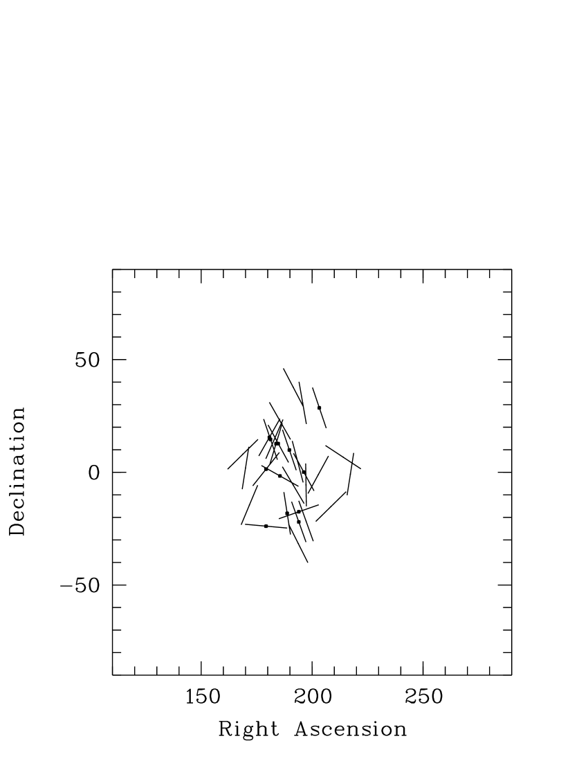
Figure 1: A map of the polarization vectors of all significantly polarized ($p\geq 0.6\%$ and $\sigma_{\theta}\leq 14\degr$) quasars with right ascensions $11^{h}15^{m}\leq\alpha\leq 14^{h}29^{m}$, and redshifts $1.0\leq z\leq 2.3$. The vector length is arbitrary. The 13 new objects are indicated by additional points

We first want to test the hypothesis that the polarization position angles of quasars located in region A1 preferentially lie in the interval [146$\degr$ – 46$\degr$] instead of being uniformly distributed. This angular sector was selected prior to the new observations –on the basis of the results of Paper I–, and the polarization position angles have been measured for a sample of quasars different from that one at the origin of the detection of the effect. Out of the 13 new significantly polarized quasars in region A1 (Table 1), 10 have their polarization position angles in the expected range. To test the null hypothesis $H_{0}$ of uniform distribution of circular observations against the alternative of sectoral preference, we may use a simple binomial test (e.g. Lehmacher & Lienert 1980, Siegel 1956). If $P_{\scriptscriptstyle\rm A}$ is the probability under $H_{0}$ that a polarization position angle falls in the angular sector [146$\degr$ – 46$\degr$], then $P_{\scriptscriptstyle\rm A}=80\degr/180\degr$. If $L$ denotes the number of polarization position angles falling in [146$\degr$ – 46$\degr$], $L$ has a binomial distribution under $H_{0}$, such that the probability to have $L_{\star}$ or more polarization angles in [146$\degr$ – 46$\degr$] is

$$P(L\geq L_{\star})=\sum_{l=L_{\star}}^{N}\left(\begin{array}[]{c}N\\ l\end{array}\right)P_{\scriptscriptstyle\rm A}^{l}\;(1-P_{\scriptscriptstyle\rm A})^{N-l}\,.$$ (1)

With $N=13$ and $L_{\star}=10$, we compute $P(L\geq 10)$ = 1.8%. This indicates that the hypothesis of uniform distribution of polarization position angles may be rejected at the 1.8% significance level in favour of coherent orientation.

A map of the quasar polarization vectors is illustrated in Fig. 1, including the objects from Paper I. An alignment is clearly seen, with a net clustering of polarization vectors around $\theta\sim 165\degr-170\degr$. Altogether, there are 29 significantly polarized quasars in this region, and 25 of them have their polarization vectors aligned i.e. their polarization position angles in the range 146$\degr$ – 46$\degr$ (Tables 1 and 2, and Paper I). It is interesting to note that the effect is stable when we increase the polarization degree cutoff (then decreasing the probability of a possible contamination): out of 22 quasars with $p\geq 0.8\%$, 19 have their polarization vectors aligned, and out of 17 quasars with $p\geq 1.0\%$, 16 have their polarization vectors aligned.

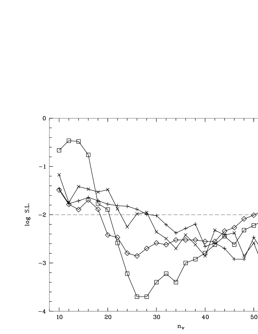
Figure 2: The logarithmic significance level (S.L.) of the four statistical tests defined in Paper I, $S$ with $\Delta\theta_{c}=60\degr$ $(\squareforqed)$, $S_{D}(\diamondsuit)$, $Z_{c}^{m}(+)$, $Z_{c}(\times)$, when applied to the new sample of 213 polarized quasars. $n_{v}$ is the number of nearest neighbours around each quasar; it is involved in the calculation of averaged quantities. The dashed horizontal line indicates the 1% significance level

Since in total 43 new polarized objects were found all over the sky, it is also interesting to re-run the global statistical tests used in Paper I. These tests are applied to the whole sample of 213 objects. The statistics basically measure the dispersion of polarization position angles for groups of $n_{v}$ neighbours in the 3-dimensional space, the significance being evaluated through Monte-Carlo simulations, shuffling angles over positions. It is not our purpose to repeat here what was done in Paper I, but only to illustrate the trend with the larger sample. The significance levels of the statistical tests, i.e. the probabilities that the test statistics would have been exceeded by chance only, are given in Fig. 2 for the four tests considered in Paper I. Compared to Figs. 9 and 10 of Paper I, all the statistical tests indicate a net decrease of the significance level for the larger sample, strengthening the view that polarization vectors are not randomly distributed over the sky but are coherently oriented in groups of 20-30 objects. We note a shift of the minimum significance level towards slightly higher values of $n_{v}$, as expected from the increase of the number density of the objects.

All these results confirm the existence of orientation effects in the distribution of quasar polarization vectors, and more particularly in the high-redshift region A1 where an independent test was performed.

4 Towards an interpretation

4.1 Observational constraints

First, it is important to note that the observational facts discussed in detail in Paper I and arguing against an instrumental bias and/or a contamination by interstellar polarization in our Galaxy are still valid. They are even strengthened since additional objects have been observed, several of them by different authors with different instrumentations. For the new measurements presented here, the polarization of field objects has been measured simultaneously and found to be very small (Lamy & Hutsemékers 2000). The comparison of the quasar polarization position angles with those of neighbouring stars has also been re-investigated for the new sample. Using the most recent compilation of Heiles (2000), we confirm the absence of correlation between quasar and Galactic star polarization angles, especially in region A1. And finally, the fact that the polarization vectors of quasars on the same line of sight but at lower redshifts are not accordingly aligned certainly remains one of the strongest arguments against artifacts.

Let us now discuss some observational results providing us with possible constraints on the phenomenon. This discussion is mostly based on quasars in region A1.

Looking at Fig. 1, we found –by chance– that the plane of the Local Supercluster (in the direction of its center) roughly passes through the structure formed by the aligned objects. We have then transformed the polarization position angles in the supergalactic coordinate system (de Vaucouleurs et al. 1991) using Eq. 16 of Paper I. A map is illustrated in Fig. 3. It shows a rough alignment of quasar polarization vectors with the supergalactic plane, the effect being more prominent for those objects close to the supergalactic equator. The most polarized objects (with $p\geq$ 5%) do follow the trend. This behavior is very reminiscent of the alignment of Galactic star polarization vectors with the Galactic plane (Mathewson & Ford 1970, Axon & Ellis 1976).

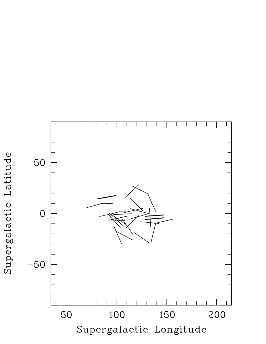
Figure 3: A map in the supergalactic coordinate system of the polarization vectors of the 29 polarized quasars belonging to region A1. The vector length is arbitrary. Thicker lines refer to objects with $p\geq 5\%$

Other constraints come from the relation between quasar intrinsic properties and polarization. In Table 2, we give all quasars in region A1 with good polarization measurements, either polarized ($p\geq 0.6\%$ and $\sigma_{\theta}\leq 14\degr$ the latter constraint being equivalent to $p/\sigma_{p}\simeq 2$), or unpolarized ($p<0.6\%$ with $\sigma_{p}\leq 0.3\%$). The quasar type is also given: broad absorption line (BAL), radio-loud non-BAL (RL), radio-quiet non-BAL (RQ), or optically selected non-BAL (O). We may first notice that the quasars with aligned polarization vectors do belong to all types, i.e. radio-quiet / optically selected (3 objects), radio-loud (9), or BAL (13). Note however that significantly polarized radio-quiet non-BAL quasars are definitely less numerous, and that two of them, B1115$+$080 and B1429$-$008, are possibly gravitationally lensed. Furthermore, we can see that the known polarization difference between BAL and non-BAL radio-quiet quasars also prevails in region A1 (Fig. 4). A Kolmogorov-Smirnov test gives a probability of only 0.6% that these two samples of are drawn from the same parent population. The illustrated distributions are also in good agreement with those reported by Hutsemékers et al. (1998). In addition, the distribution of $p$ for non-BAL radio-quiet quasars is very similar to that found by Berriman et al. (1991) for the Palomar-Green quasar sample. This clearly indicates that, also in region A1, quasar polarization is related to the intrinsic properties of the objects.

Table 2: Polarized and unpolarized quasars in region A1

Object	$z$	$p$	$\sigma_{p}$	$\theta$	$\sigma_{\theta}$	Ref	Type
(B1950)		(%)	(%)	($\degr$)	($\degr$)
B1115$+$080	1.722	0.68	0.27	46	12	0	RQ
B1120$+$019	1.465	1.95	0.27	9	4	0	BAL
B1127$-$145	1.187	1.26	0.44	23	10	2	RL
B1138$-$014	1.270	0.38	0.23	53	21	9	BAL
B1138$+$040	1.876	0.10	0.24	36	-	1	RQ
B1157$-$239	2.100	1.33	0.17	95	4	9	BAL
B1157$+$014	1.990	0.76	0.18	39	7	9	RL
B1158$+$007	1.380	0.44	0.20	74	14	9	RL
B1203$+$155	1.630	1.54	0.20	30	4	9	BAL
B1205$+$146	1.640	0.83	0.18	161	6	9	BAL
B1206$+$459	1.158	0.24	0.17	132	20	1	RQ
B1210$+$197	1.240	0.33	0.19	76	19	9	RL
B1212$+$147	1.621	1.45	0.30	24	6	0	BAL
B1215$+$127	2.080	0.62	0.24	17	12	9	BAL
B1216$+$110	1.620	0.58	0.19	63	10	9	BAL
B1219$+$127	1.310	0.68	0.20	151	9	9	BAL
B1222$-$016	2.040	0.80	0.22	119	8	9	BAL
B1222$+$146	1.550	0.23	0.18	65	30	9	O
B1222$+$228	2.046	0.84	0.24	150	8	2	RL
B1225$+$317	2.200	0.16	0.24	150	-	2	RL
B1228$+$122	1.410	0.12	0.18	142	-	9	BAL
B1230$-$237	1.840	0.05	0.19	72	-	9	O
B1230$+$170	1.420	0.30	0.19	101	22	9	BAL
B1234$-$021	1.620	0.54	0.18	72	10	9	O
B1235$-$182	2.190	1.02	0.18	171	5	9	RL
B1238$-$097	2.090	0.18	0.18	80	-	9	O
B1239$+$099	2.010	0.82	0.18	161	6	9	BAL
B1239$+$145	1.950	0.18	0.20	21	-	9	RQ
B1241$+$176	1.273	0.12	0.19	120	-	1	RL
B1242$+$001	2.080	0.22	0.19	56	39	9	RQ
B1246$-$057	2.236	1.96	0.18	149	3	8	BAL
B1246$+$377	1.241	1.71	0.58	152	10	2	RL
B1247$+$267	2.038	0.41	0.18	97	12	1	RQ
B1248$+$401	1.030	0.20	0.19	3	-	1	RQ
B1250$+$012	1.690	0.21	0.18	132	37	9	BAL
B1254$+$047	1.024	1.22	0.15	165	3	1	BAL
B1255$-$316	1.924	2.20	1.00	153	12	4	RL
B1256$-$220	1.306	5.20	0.80	160	4	7	RL
B1256$-$175	2.060	0.91	0.19	71	6	9	RL
B1258$-$164	1.710	0.53	0.18	132	10	9	O
B1303$+$308	1.770	1.12	0.56	170	14	3	BAL
B1305$+$001	2.110	0.70	0.22	151	9	9	O
B1309$-$216	1.491	12.30	0.90	160	2	4	RL
B1309$-$056	2.212	0.78	0.28	179	11	0	BAL
B1317$+$277	1.022	0.15	0.20	94	-	2	RQ
B1329$+$412	1.930	0.36	0.21	83	16	1	RQ
B1331$-$011	1.867	1.88	0.31	29	5	0	BAL
B1333$+$286	1.910	5.88	0.20	161	1	9	BAL
B1334$+$262	1.880	0.23	0.19	116	34	9	BAL
B1338$+$416	1.219	0.37	0.19	67	15	1	RQ
B1354$-$152	1.890	1.40	0.50	46	10	4	RL
B1416$+$067	1.439	0.77	0.39	123	14	2	RL
B1429$-$008	2.084	1.00	0.29	9	9	0	RQ
B1429$-$006	1.180	0.07	0.20	107	-	9	BAL

References: (0) Hutsemékers et al. 1998, (1) Berriman et al. 1990, (2) Stockman et al. 1984, (3) Moore & Stockman 1984, (4) Impey & Tapia 1990, (7) Visvanathan & Wills 1998, (8) Schmidt & Hines 1999, (9) Lamy & Hutsemékers 2000

4.2 Discussion

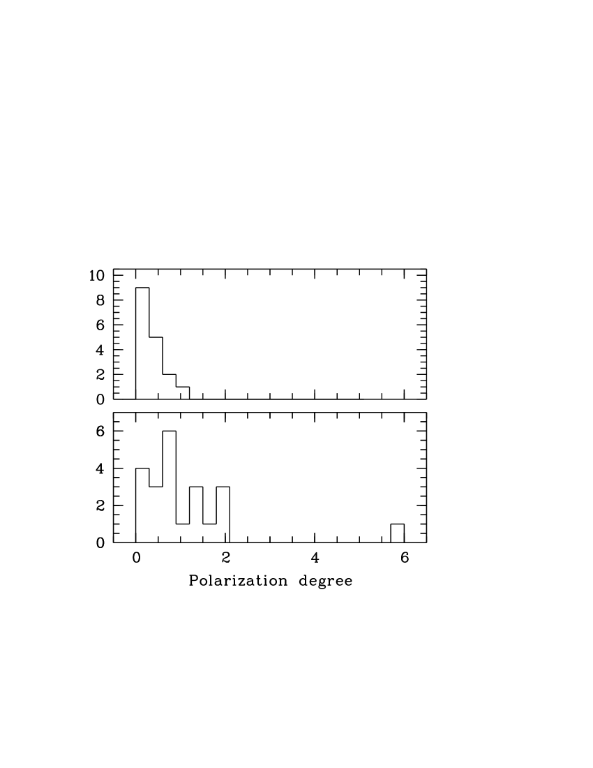
Figure 4: The distribution of the polarization degree $p$ (in %) for the quasars located in the region of alignment A1 (Table 2). Upper panel: radio-quiet (RQ+O) quasars. Lower panel: BAL quasars

The apparent alignment of quasar polarization vectors with the supergalactic plane is very appealing as the starting point of an explanation, namely since this could decrease by more than one order of magnitude the scale at which a mechanism must act coherently. By analogy with the alignment of stellar polarization vectors with the plane of our Galaxy (Mathewson & Ford 1970, Axon & Ellis 1976), some dichroism could be achieved due to extinction by dust grains aligned in a magnetic field. Another possibility could be the conversion of photons into pseudo-scalars also within a magnetic field (Harari & Sikivie 1992, Gnedin & Krasnikov 1992, Gnedin 1994). In both cases the hypothetical magnetic field should be coherent on a $\sim$50 Mpc scale, which is only slightly larger than the large-scale magnetic field possibly detected by Vallée (1990) in the direction of the Virgo cluster. But this interpretation suffers some drawbacks: namely, it cannot explain why the polarization vectors of quasars at lower redshifts are not accordingly aligned (cf. Fig. 5 in Paper I).

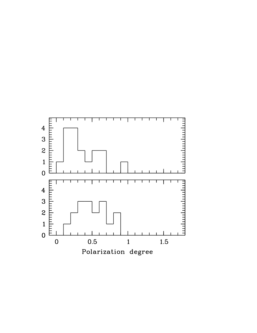
Figure 5: The distribution of the polarization degree for the radio-quiet (RQ+O) quasars in region A1. The upper panel is an enlargement of that of Fig. 4 and refers to the observed polarization degree $p$ (in %). The so-called polarization bias (due to the fact that $p$ is always a positive quantity) affects the first bin (see also Berriman et al. 1991). The lower panel shows the distribution of the polarization degree after subtraction of a small but systematic polarization ($p_{s}=0.25\%$, $\theta_{s}=170\degr$)

It is therefore difficult to escape the conclusion that if a mechanism is able to produce the alignment of polarization vectors of high-redshift quasars by modifying the polarization state of photons during their travel towards us, this must happen at redshifts $z\ga 1$ (for region A1), or all along the line of sight assuming a cumulative or oscillatory effect (see also discussion in Paper I). Interestingly, an oscillation of quasar polarization with cosmological distance has been predicted as the consequence of the conversion of photons into pseudo-scalars within a large-scale magnetic field permeating the intergalactic medium (Harari & Sikivie 1992, Gnedin & Krasnikov 1992, Gnedin 1994). However, this interpretation, like other mechanisms which affect light as it propagates towards us, cannot easily explain why correlations observed between quasar polarization and intrinsic properties are not washed away.

In this view we may ask ourselves how small could be the systematic polarization which, added to randomly oriented polarization vectors, can be at the origin of an orientation effect which involves nearly all polarized quasars of region A1. To simulate this, we have vectorially subtracted a systematic polarization $p_{s}$ oriented at $\theta_{s}=170\degr$ (the dominant direction, cf. Fig. 1) from all polarized and unpolarized quasars of region A1 (Table 2). Then we have re-selected a sample of significantly polarized quasars with the conditions $p\geq 0.6\%$ and $\sigma_{\theta}\leq 14\degr$. For $p_{s}=0.25\%$, 29 quasars fulfil the conditions and only 15 objects out of this new sample have their polarization position angles still in the range $146\degr-46\degr$. This small systematic polarization seems therefore sufficient to produce the orientation effect, and small enough to preserve the difference between BAL and non-BAL quasars. However, as seen in Fig. 5, even such a small systematic polarization significantly modifies the polarization distribution of non-BAL radio-quiet quasars which appears depleted at polarization degrees $p\la p_{s}$, and then quite different from the distribution found by Berriman et al. (1991) and Hutsemékers et al (1998). If we further note that values of $p_{s}$ higher than 0.25% are obviously needed to explain the alignment of the 16 objects with $p\geq 1.0\%$, we may conclude that it is quite difficult to invoke a systematic additional polarization along the line of sight without modifying the quasar intrinsic polarization properties. This simple test also provides additional evidence that a systematic instrumental effect is unlikely.

Although more subtle and speculative effects modifying the polarization of light along the line of sight can probably be imagined, we may admit on the other hand that the quasars themselves i.e. their structural axes are coherently oriented on Gpc scales. For radio-loud quasars, it is well known that the optical polarization is often parallel to the structural axis of the radio core (Rusk 1990, Impey et al. 1991). Unfortunately, only one polarized quasar in region A1 (B1127$-$145) is spatially resolved. It is however very interesting to note that this object has a core structure parallel to its polarization vector (Impey & Tapia 1990). In this view it is worth noting that possible coherence of morphological structures from the central engines of active galactic nuclei to superclusters has been suggested by West (1991, 1994), although this observation is apparently not confirmed at the supercluster scale (Jaaniste et al. 1998). From the theoretical point of view, some studies (Reinhardt 1971, Wasserman 1978) have pointed out the possible effects of magnetic fields on galaxy formation and orientation. Extrapolating, a correlation between quasar structural axes could be settled at the epoch of formation and related to very large-scale primordial magnetic fields possibly formed during inflation (Battaner & Florido 2000). Large-scale vorticity is another possibility, at least qualitatively. In this view, the apparent alignment found with the supergalactic plane is puzzling. However, coincidence cannot be ruled out, especially if we note that the polarization vectors of quasars belonging to the other regions of alignments (regions A2 and A3 in Paper I) do not show the same alignment with the plane of the Local Supercluster.

5 Conclusions

In order to verify the existence of very large-scale coherent orientations of quasars polarization vectors, we have obtained new polarization measurements for quasars located in a given region of the sky where the range of polarization position angles was predicted in advance. The statistical analysis of this new sample provides an independent confirmation of the existence of alignments of quasar polarization vectors at high redshifts. In total, out of 29 polarized quasars located in this region, 25 have their polarization vectors coherently oriented. Moreover, global statistical tests applied to the whole sample indicate that, with the increased size of the sample, the detection of the effect is stable and even more significant.

The increased size of the sample also allowed us to put some constraints on the phenomenon. We namely found that the polarization vectors of quasars in region A1 are apparently parallel to the plane of the Local Supercluster, while those of quasars at lower redshifts are not accordingly aligned. Furthermore, we found that the well-known correlations between quasar intrinsic properties and polarization also prevail for those quasars located in that region of alignment.

Mechanisms modifying the polarization somewhere along the line of sight could explain some results, but cannot easily fit all constraints, namely the fact that correlations between quasar intrinsic properties and polarization are not washed away. Another possibility is that the quasar structural axes themselves are coherently oriented. However, given the scales involved, a reasonable physical mechanism is far from obvious. Interestingly, in region A1, nine quasars with aligned polarization vectors are radio-loud, such that this hypothesis could be tested by simply mapping their radio core.

The interpretation of this orientation effect therefore remains puzzling. Nevertheless, the presence of coherent orientations at such large scales seems to indicate the existence of a new interesting effect of cosmological importance.

- (1) Axon D.J., Ellis R.S. 1976, MNRAS 177, 499
- (2) Battaner E., Florido E. 2000, ASP Conf. Series 200, 144
- (3) Berriman G., Schmidt G.D., West S.C., Stockman H.S. 1990, ApJS 74, 869
- (4) Brotherton M.S., van Breugel W., Smith R.J. et al. 1998, ApJ 505, L7
- (5) de Vaucouleurs G., de Vaucouleurs A., Corwin H.G. et al. 1991, Third Reference Catalogue of Bright Galaxies, Springer-Verlag
- (6) Gnedin Y.N., Krasnikov S.V. 1992, Sov. Phys. JETP 75, 933
- (7) Gnedin Y.N. 1994, Astron. Astrophys. Transactions 5, 163
- (8) Harari D., Sikivie P. 1992, Phys. Lett. B 289, 67
- (9) Heiles C. 2000, AJ 119, 923
- (10) Hewitt A., Burbidge G. 1993, ApJS 87, 451
- (11) Hutsemékers D. 1998, A&A 332, 410 (Paper I)
- (12) Hutsemékers D., Lamy H. & Remy M. 1998, A&A 340, 371
- (13) Hutsemékers D., Lamy H. 2000, A&A 358, 835
- (14) Impey C.D., Tapia S. 1990, ApJ 354, 124
- (15) Impey C.D., Lawrence C.R., Tapia S. 1991, ApJ 375, 46
- (16) Jaaniste J., Tago E., Einasto M. et al. 1998, A&A 336, 35
- (17) Lamy H., Hutsemékers D. 2000, A&AS 142, 451
- (18) Lehmacher W., Lienert G.A. 1980, Biom. J. 22, 249
- (19) Mathewson D.S., Ford V.L. 1970, Mem. R. Ast. Soc. 74, 139
- (20) Moore R.L., Stockman H.S. 1984 ApJ 279, 465
- (21) Reinhardt M. 1971, Ap&SS 10, 363
- (22) Rusk R. 1990, J. R. Astron. Soc. Can. 84, 199
- (23) Schmidt G.D., Hines D.C. 1999, ApJ 512, 125
- (24) Siegel S. 1956, Nonparametric Statistics, McGraw-Hill
- (25) Stockman H.S., Moore R.L., Angel J.R.P. 1984, ApJ 279, 485
- (26) Vallée J.P. 1990, AJ 99, 459
- (27) Véron-Cetty M.P., Véron P. 1998, ESO Scientific Report 18
- (28) Visvanathan N., Wills B.J. 1998, AJ 116, 2119
- (29) Wasserman I. 1978, ApJ 224, 337
- (30) West M.J. 1991, ASP Conf. Series 21, 290
- (31) West M.J. 1994, MNRAS 268, 79