The 2dF Galaxy Redshift Survey: The Number and Luminosity Density of Galaxies

Abstract

We present the bivariate brightness distribution (BBD) for the 2dF Galaxy Redshift Survey (2dFGRS) based on a preliminary subsample of 45,000 galaxies. The BBD is an extension of the galaxy luminosity function incorporating surface brightness information. It allows the measurement of the local luminosity density, $j_{B}$, and the galaxy luminosity and surface brightness distributions while accounting for surface brightness selection biases.

The recovered 2dFGRS BBD shows a strong surface brightness-luminosity relation ($M_{B}\propto(2.4\pm^{1.5}_{0.5})\mu_{e}$) providing a new constraint for galaxy formation models. In terms of the number-density we find that the peak of the galaxy population lies at $M_{B}\geq-16.0$ mag. Within the well defined selection limits ($-24<M_{B}<-16.0$ mag, $18.0<\mu_{e}<24.5$ mag arcsec^-2) the contribution towards the luminosity-density is dominated by conventional giant galaxies (i.e. 90% of the luminosity-density is contained within $-22.5<M<-17.5$, $18.0<\mu_{e}<23.0$). The luminosity-density peak lies away from the selection boundaries implying that the 2dFGRS is complete in terms of sampling the local luminosity-density and that luminous low surface brightness galaxies are rare. The final value we derive for the local luminosity-density, inclusive of surface brightness corrections, is: $j_{B}=2.49\pm 0.20\times 10^{8}h_{100}$L_⊙Mpc^-3. Representative Schechter function parameters are: M${}^{*}=-19.75\pm 0.05$, $\phi^{*}=2.02\pm 0.02\times 10^{-2}$ and $\alpha=-1.09\pm 0.03$. Finally we note that extending the conventional methodology to incorporate surface brightness selection effects has resulted in an increase in the luminosity-density of $\sim 37$%. Hence surface brightness selection effects would appear to explain much of the discrepancy between previous estimates of the local luminosity density.

1 Introduction

Of paramount importance in determining the mechanism(s) and epoch(s) of galaxy formation (as well as the local luminosity density), is the accurate and detailed quantification of the local galaxy population. It represents the benchmark against which both environmental and evolutionary effects can be measured. Traditionally this research area originated with the all-sky photographic surveys coupled with a few handfuls of hard earned redshifts. Over the past decade this has been augmented by both CCD-based imaging surveys and multi-slit/fibre-fed spectroscopic surveys. From these data, a number of perplexing problems have arisen, most notably: the faint blue galaxy problem (Koo & Kron 1992; Ellis 1997), the local normalisation problem (Maddox et al. 1990; Shanks 1990; Driver, Windhorst & Griffiths 1995; Marzke et al. 1998), the cosmological significance of low surface brightness galaxies (Disney 1976; McGaugh 1996; Sprayberry et al. 1996; Dalcanton et al. 1997; Impey & Bothun 1997) and dwarf galaxies (Babul & Rees 1992; Phillipps & Driver 1995; Loveday 1997; Babul & Ferguson 1996). These issues largely remain unresolved and arguably await an improved definition of the local galaxy population (Driver 1999).

Recent advancements in technology now allow for wide field-of-view CCD imaging surveys and bulk redshift surveys through purpose built multi-fibre spectrographs such as the common-user two-degree field (2dF) facility at the Anglo Australian Telescope (Taylor, Cannon & Parker 1998). The Sloan Digital Sky Survey elegantly combines these two facets (Margon 1999).

The quantity and quality of data that is becoming available allows not only the revision of earlier results but more fundamentally the opportunity to review and enhance the methodology with which the local galaxy population is represented. For instance some criticism that might be levied at the current methodology — the representation of the space density of galaxies using the Schechter Luminosity function (Schechter 1976; Felten 1985; Binggeli, Sandage & Tammann 1988) — is that firstly, it assumes that galaxies are single parameter systems defined by their apparent magnitude alone, and secondly it describes the entire galaxy population by only three parameters; the characteristic luminosity $L_{*}$, the normalisation of the characteristic luminosity $\phi_{*}$, and the faint-end slope $\alpha$. While it is desirable to represent the population with the minimum number of parameters, important information may lie in the nuances of detail.

In particular, two recent areas of research suggest a greater diversity in the galaxy population than is allowed by the Schechter function form. Firstly, Marzke et al. (1994) and also Loveday (1997) report the indication of a change in the faint end slope at faint absolute magnitudes — a possible giant-dwarf transition — and this is also seen in a number of Abell clusters where it is easier to probe into the dwarf regime (e.g., Driver et al. 1994; De Propris et al. 1995; Driver, Couch & Phillipps 1998; Trentham 1998). Secondly a number of studies show that the three Schechter parameters, and in particular the faint-end slope, have a strong dependence upon: surface brightness limits (Sprayberry, Impey & Irwin 1996; Dalcanton 1998); colour (Lilly et al. 1996); spectral type (Folkes et al. 1999); optical morphology (Marzke et al. 1998), environment (Phillipps et al. 1998) and wavelength (Loveday 2000). It has been noted (Willmer 1997) that the choice of method for reconstructing the galaxy LF also contains some degree of bias.

More fundamentally, evidence that the current methodology might actually be flawed comes from comparing recent measurements of the galaxy luminosity function as shown in Fig. 1. The discrepancy between these surveys is significantly adrift from the quoted formal errors implying an unknown systematic error. The range of discrepancy can be quantified as a factor of 2 at the $L_{*}$ ($M\sim-19.5$) point rising to a factor of 10 at $0.01L_{*}$ ($M\sim-14.5$). The impact of this variation is a factor of 3-4, for instance, in assessing the contribution of galaxies to the local baryon budget (e.g. Persic & Salucci 1992; Bristow & Phillipps 1994; and Fukugita, Hogan & Peebles 1998).

Figure 1: Schechter luminosity functions from recent magnitude-limited redshift surveys (q.v. Table 1). The line becomes dotted outside the range of survey data. The range of values show the uncertainty in the LF which in turn filters through to the local measure of the mean luminosity density.

This uncertainty is in addition to that introduced from the unanswered question of the space density of low surface brightness galaxies. The most recent attempt to quantify this is by O’Neil & Bothun (2000) — following on from McGaugh (1996), and in turn Disney (1976) — who conclude that the surface brightness function (SBF) of galaxies — the number density of galaxies in intervals of surface brightness — is of similar form to the luminosity function. Thus both the LF and SBF are described by a flat distribution with a cutoff at bright absolute magnitudes or high surface brightnesses. Taking the O’Neil result at face value, this implies a further error in measures of the local luminosity density of 2-3 - i.e. the contribution to the luminosity- (and hence baryon-) density from galaxies is uncertain to a factor of $\sim 10$. However the significance of low surface brightness galaxies depends upon their luminosity range and similarly the completeness of the LF relies on the surface brightness intervals over which each luminosity bin is valid. Both representations are incomplete unless the information is combined. This leads us to the conclusion that both the total flux and the manner in which this flux is distributed must be dealt with simultaneously. Several papers have been published which deal with either surface brightness distributions or Bivariate Brightness Distributions (Phillipps & Disney 1986, Boyce & Phillipps 1994, Minchin 1999, Sodre & Lahav 1993, and Petrosian 1998). These are either theoretical, limited to cluster environments or have poor statistics due to the scarcity of good redshift data.

Recently, Driver (1999) determined the first measure of the bivariate brightness distribution for field galaxies using Hubble Deep Field data (Williams et al. 1996) and capitalising on photometric redshifts (Fernández-Soto et al. 1998). The result, based on a volume limited sample of 47 galaxies, implied that giant low surface brightness galaxies were rare but that there exists a strong Luminosity-Surface Brightness relationship, similar to that seen in Virgo (Binggeli 1993). The sense of the relationship implied that low surface brightness galaxies are preferentially of lower luminosity (i.e. dwarfs). If this is borne out it strongly tempers the conclusions of O’Neil & Bothun (2000). While the number of low surface brightness galaxies may be large, their luminosities are low, so their contribution to the local luminosity density, is also low, $<20$% (Driver 1999).

This paper attempts to bundle these complex issues onto a more intuitive platform by expanding the current representation of the local galaxy population to allow for: surface brightness detection effects, star-galaxy separation issues, surface brightness photometric corrections and clustering effects. This is achieved by expanding the mono-variate luminosity function into a bivariate brightness distribution (BBD) where the additional dimension is surface brightness. The 2dFGRS allows us to do this for the first time by having a large enough database to separate galaxies in both magnitude and surface brightness without having too many problems with small number statistics.

In §2 we discuss the revised methodology for measuring the space density of the local galaxy population, the local luminosity density and the contribution towards the baryon density in detail. In §3 we present the current 2dFGRS data (containing $\sim 45,000$ galaxies or one fifth of the expected final tally). In §4 we correct for the light lost under the isophote and define our surface brightness measure. In §5 we apply the methodology to construct the first statistically significant bivariate brightness distribution for field galaxies. The results for the number-density and luminosity-density are detailed in §6 and §7. In §8, we compare these results to other surveys. Finally we present our conclusions.

Throughout we adopt $H_{o}=100$kms^-1Mpc^-1 and a standard flat cosmology with zero cosmological constant (i.e. $q_{o}=0.5,\Lambda=0$). However we note that the results presented here are only weakly dependent on the cosmology.

2 Methodology

The luminosity density, $j$, is the total amount of flux emitted by all galaxies per Mpc³. When measured in the UV band it can be converted to a measure of the star-formation rate (see for example Lilly et al. 1996, Madau et al. 1998). When measured at longer wavelengths it can be combined with mass-to-light ratios to yield an approximate value for the contribution from galaxies towards the local matter density $\Omega_{M}$ — independent of $H_{o}$, only weakly cosmology dependent and not reliant on any specific theory of structure formation (see for example Carlberg et al. 1996; Fukugita, Hogan & Peebles 1998). The two main caveats are firstly the accuracy of $j_{B}$ (the luminosity density measured in the B-band), and secondly the assumption of a ubiquitous mass-to-light ratio.

2.1 Measuring $j$

The luminosity density, $j$, is found by integrating the product of the number density $\Phi(L/L_{*})$ and the luminosity L with respect to luminosity.

$$j=\int^{\infty}_{0}L\,\Phi(L/L_{*})\,d(L/L_{*})$$ (1)

By convention, $j$ is typically derived from a magnitude-limited redshift survey by determining the representative Schechter parameters for a survey (e.g. Efstathiou et al. 1988) and then integrating the luminosity weighted Schechter function, where $\Phi(L/L_{*})\,d(L/L_{*})$ is the Schechter function (Schechter 1976) given by:

$$\Phi(L/L_{*})\,d(L/L_{*})=\phi_{*}\,(L/L_{*})^{\alpha}\,\exp{[-(L/L_{*})]}\,d(L/L_{*})$$ (2)

and $\phi_{*},L_{*},$ and $\alpha$ are the three parameters which define the survey (referred to as the normalisation point, characteristic turn-over luminosity and faint-end slope parameter respectively). More simply if a survey is defined by these three parameters it follows that:

$$j=\phi_{*}\,L_{*}\,\Gamma(\alpha+2)$$ (3)

Table 1 shows values for the luminosity density derived from a number of recent magnitude-limited redshift surveys (as indicated). The variation between the measurements of $j$ from these surveys is $\sim 2$ and hence the uncertainty in the galaxy contribution to the mass budget is at best equally uncertain. This could be due to a number of factors, e.g., large scale-structure, selection biases, redshift errors, photometric errors or other incompleteness. In this paper we wish to explore the possibility of selection bias due to surface brightness considerations only. The principal motivation for this is that the LCRS (lower line on Fig. 1), which recovers the lowest $j$ value, adopted a bright isophotal detection limit of $\mu_{r}=23$ mag arcsec^-2, suggesting a dependence between the measured $j$ and the surface brightness limit of the survey. Here we develop a method for calculating $j$ which incorporates a number of corrections/considerations for surface brightness selection biases. In particular, a surface brightness dependent Malmquist correction, a surface brightness redshift completeness correction and an isophotal magnitude correction. We also correct for clustering. What is not included here, and will be pursued in a later paper, is the photometric accuracy, star-galaxy separation accuracy and a detection correction specifically for the two degree field galaxy redshift survey (2dFGRS).

Implementing these corrections requires re-formalising the path to $j$. Firstly, we replace the luminosity function representation of the local galaxy population by a bivariate brightness distribution (BBD). The bivariate brightness distribution is the galaxy number density, $\Phi$, as a function of absolute, total, B-band magnitude, $M_{B}$, and absolute, effective surface brightness, $\mu_{e}$, i.e., $\Phi(M,\mu)$. To construct a BBD we need to convert the observed distribution to a number density distribution taking into account the Malmquist bias and the redshift incompleteness correction, i.e.,

$$\Phi(M,\mu)=\frac{O(M,\mu)+I(M,\mu)}{V(M,\mu)}\,W(M,\mu)$$ (4)

where:

• $O(M,\mu)$ is the matrix of absolute magnitude, $M$, and absolute effective surface brightness, $\mu$, for galaxies with redshifts.

• $I(M,\mu)$ is the matrix of absolute magnitude, $M$, and absolute effective surface brightness, $\mu$, for those galaxies for which redshifts were not obtained.

• $V(M,\mu)$ is the matrix which specifies the volume over which a galaxy with absolute magnitude, $M$, and absolute effective surface brightness, $\mu$, can be seen (see also Phillipps, Davies & Disney 1990).

• $W(M,\mu)$ is the matrix that weights each bin to compensate for clustering.

Deriving these matrices is discussed in detail later. $j$ is then defined as:

$$j=\sum^{M}\sum^{\mu}L(M)\,\Phi(M,\mu)$$ (5)

or in practice,

$$j=\sum^{M}\sum^{\mu}10^{-0.4(M-M_{\odot})}\,\Phi(M,\mu)$$ (6)

in units of $L_{\odot}$Mpc^-3 where $M_{\odot\,\rm B}=5.48$.

Our formalism has two key advantages over the traditional luminosity function: Firstly, it adds the additional dimensionality of surface brightness allowing for surface brightness specific corrections. Secondly, it represents the galaxy population by a distribution rather than a function, thus requiring no fitting procedures or assumption of any underlying parametric form.

3 The Data

The data set presented here is based upon a sub-sample of the Automated Plate Measuring-machine galaxy catalogue (APM; Maddox et al. 1990a,b) for which spectra have been obtained using the two-degree field Facility (2dF) at the Anglo-Australian Telescope (AAT).

The original APM catalogue contains $b_{J}$ magnitudes with random error $\Delta m=\pm 0.2$ mag (Folkes et al. 1999) and isophotal areas $A_{\rm ISO}$. The isophotal area is defined as the number of pixels above a limiting isophote, $\mu_{\rm lim}$ — set at the $2\sigma$ level above the sky background ($\mu_{lim}\approx 24.53$ mag arcsec^-2 with a variation of $\pm 0.11$ mag arcsec^-2 - Pimbblet et al. 2000). However APM $b_{J}$ magnitudes are found to vary from CCD $b_{J}$ magnitudes by $0.14\pm 0.29$mag (Metcalfe et al. 1995). Therefore the isophotal limit in APM $b_{J}$ magnitudes is $\mu_{lim}=24.67\pm 0.30$mag arcsec^-2. One pixel equals 0.25 $\Box^{\prime\prime}$. The minimum isophotal area found for galaxies in the APM catalogue is 35$\Box^{\prime\prime}$. Star-galaxy separation was implemented as described in Maddox et al. (1990b). The final APM sample contains $3\times 10^{6}$ galaxies covering 15,000 square degrees – see Maddox et al. (1990a,b) for further details.

The 2dFGRS input catalogue is a 2000 $\Box^{o}$ subregion of the APM catalogue (covering two continuous regions in the northern and southern Galactic caps plus random fields) with an extinction corrected magnitude limit of $m=19.45$ (Colless 1999). The input catalogue contains 250,000 galaxies for which 81,895 have been observed using 2dF (as of November 1999). Each spectrum within the database has been examined by eye to check if the redshift is reliable. Redshifts are determined via cross-correlation with specified templates (see Folkes et al. 1999 for details). A brief test of the reliability of the 2dFGRS was achieved via a comparison between 1404 galaxies in common with the Las Campanas Redshift Survey (Lin et al. 1996) for which there were only 8 mismatches, showing that 2dF redshifts are reliable. Of the 81,895 galaxies, 74,562 have a redshift, resulting in a redshift completeness of 91%.

The survey comprises many overlapping two degree fields and many still have to be observed. Hence the absolute normalisation is tied to the full input galaxy catalogue which is known to contain 174.0 galaxies with $m\leq 19.45$ per square degree. Using a subsample of 44796 galaxies, covering just the South Galactic Pole (SGP) region, this yields an effective coverage for this survey of 257 non-contiguous square degrees.

Finally, for the purposes of this paper, we adopt a lower redshift limit of $z=0.015$ to minimise the influence of peculiar velocities in the determination of absolute parameters and an upper redshift limit of $z=0.12$.

This upper limit of $z=0.12$ was selected so as to maximise the sample size yet minimise the error introduced by the isophotal corrections. At $z=0.12$ the uncertainty in the isophotal correction ($\pm^{0.07}_{0.16}$), due to type uncertainty (see Appendix A), remains smaller than the photometric error ($\pm 0.2$ mags). Note that the increase in the error in the isophotal correction is primarily because of the increase in the intrinsic isophotal limit due to a combination of surface brightness-dimming and the K-correction.

The final sample is therefore pseudo volume-limited and contains 20,765 galaxies, with redshifts, selected from a parent sample of 45,000.

Note: all magnitude and surface brightnesses are in the APM $b_{j}$ filter.

4 Isophotal corrections

The APM magnitudes have already been corrected assuming a Gaussian profile (see Maddox et al. 1990b for full details). This was aimed primarily at recovering the light lost due to the seeing and is crucial for compact objects. It is known to significantly underestimate the isophotal correction required for low surface brightness disks. Such systems typically exhibit exponential profiles with disks which can extend a substantial distance beyond the isophote, the most famous example being Malin 1 (Bothun et al. 1987). Once thought of as a Virgo dwarf this system remains the most luminous field galaxy known.

To compliment the Gaussian correction (required for compact objects but ineffectual for extended sources) we introduce an additional correction (ineffectual for compact sources but suitable for extended disks). This correction assumes all objects can be represented by a pure exponential surface brightness profile extending from the core outwards. In this case the surface brightness profile is simply:

$$\Sigma(r)=\Sigma_{o}\exp(-r/\alpha)$$ (7)

or,

$$\mu(r)=\mu_{o}+1.086(r/\alpha)$$ (8)

Where $\Sigma_{o}$ is the central surface brightness in Wm^-2 arcsec^-2, $\alpha$ is the scale length of the galaxy in arcsecs and r the radius in arcsecs. $\mu_{o}$ is the central surface brightness in mag arcsec^-2.

Under this assumption a galaxy’s observed isophotal luminosity is the integrated radial profile out to $r_{iso}$.

$$l_{iso}=2\pi\int^{r_{iso}}_{0}\Sigma_{o}\exp(-r/\alpha)rdr$$ (9)

which can be expressed in magnitudes as:

$$m_{iso}=\mu_{o}^{app}-2.5\log_{10}\{2\,\pi[\alpha^{2}-\alpha(\alpha+r_{iso})\exp(-r_{iso}/\alpha)]\}$$ (10)

(here $\mu^{app}_{o}$ denotes the apparent surface brightness uncorrected for redshift.) $\mu_{lim}$, the detection/photometry isophote, can be expressed as:

$$\mu_{lim}=\mu_{o}^{app}+1.086(r_{iso}/\alpha)$$ (11)

As $m_{iso}$, $r_{iso}$ and $\mu_{lim}$ are directly measurable quantities, equations ( 10 &  11 ) can be solved numerically. The total magnitude is then given by:

$$l_{tot}=2\pi\int^{\infty}_{0}\Sigma_{o}\exp(-r/\alpha)rdr=2\pi\Sigma_{o}\alpha^{2}$$ (12)

or,

$$m^{tot}=\mu_{o}^{app}-2.5\log_{10}(2\pi\alpha^{2})$$ (13)

From this description an extrapolated central surface brightness can be deduced numerically from the specified isophotal area and isophotal magnitude (after the seeing correction). Note that this prescription ignores the possible presence of a bulge, opacity, and inclination leading to an underestimate of the isophotal correction. This is unavoidable as the data quality is insufficient to establish bulge-to-disk ratios. To verify the impact of this we explore the accuracy of the isophotal correction for a variety of galaxy types in Appendix A. The tests show that the isophotal correction is a significant improvement over the isophotal magnitudes for all types - apart for ellipticals where the introduced error is negligible compared to the photometric error - and a dramatic improvement for low surface brightness systems. The final magnitudes, after isophotal correction, now lie well within the quoted error of $\pm 0.2$ mags for both high- and low-surface brightness galaxies.

4.1 The Effective Surface Brightness

Most results cited in the literature use the central surface brightness or the effective surface brightness. The central surface brightness, as described above, is the extrapolated surface brightness at the core under the assumption of a perfect exponential disk. The effective surface brightness is the mean surface brightness within the half-light radius. The conversion between the measures is relatively straightforward and described as follows:

$$l_{\frac{1}{2}}=\pi\,\Sigma_{o}\,\alpha^{2}=2\pi\,\Sigma_{o}\,\alpha^{2}[1-(1+r_{e}/\alpha)\exp(-r_{e}/\alpha)]$$ (14)

which can be solved numerically to get

$$r_{e}=1.678\alpha$$ (15)

The effective surface brightness is now given by:

$$\mu_{e}^{app}=\mu_{o}^{app}+2.5\log_{10}[(r_{e}/\alpha)^{2}]=\mu_{o}^{app}+1.124$$ (16)

Hence from the isophotal magnitudes and areas we can derive the total magnitude and effective surface brightness (quantities which are now independent of the isophotal detection threshold). We chose to work with effective surface brightness as it can, at some later stage, be measured directly from higher quality CCD data. Note that these surface brightness measures are all apparent rather than intrinsic, however this is not important as although surface brightness is distance dependent the isophotal correction is not (this is because both $\mu_{lim}$ and $\mu_{e}$ vary with redshift in the same way).

Fig. 2 shows the final 2dFGRS sample (i.e. after isophotal correction) for those galaxies with (upper panel) and without (lower panel) redshifts. The galaxies are plotted according to their apparent total magnitude and apparent effective surface brightness. The curved boundary at the faint end of both plots is due to the isophotal corrections which are strongly dependent on $\mu_{e}$ for a constant $m$. As $\mu_{e}-1.124$ tends towards $\mu_{lim}$, the isophotal limit, the correction tends towards infinity, making it impossible to see galaxies close to $\mu_{lim}$. The average isophotal correction is $0.33$ mag (for $\mu_{lim}=24.67$ mag arcsec^-2).

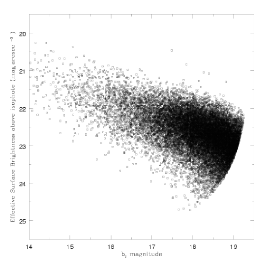
Figure 2: Galaxies with (upper) and without (lower) redshifts for the current 2dFGRS sample plotted according to their apparent extinction corrected total magnitude and apparent effective surface brightness.

The observed mean magnitude and observed mean effective surface brightness for those galaxies with and without redshifts are: $18.06\pm 0.01$ mag & $22.66\pm 0.01$ mag arcsec^-2 and $18.54\pm 0.01$ mag & $23.17\pm 0.01$ mag arcsec^-2, respectively. These figures imply that galaxies closer to the detection limits are preferentially under-sampled.

5 Constructing the BBD

We now apply the methodology described in section 2 to derive the BBD from our data set. This requires constructing the four matrices, $O(M,\mu)$, $I(M,\mu)$, $V(M,\mu)$ and $W(M,\mu)$.

5.1 Deriving $O(M,\mu)$

For those galaxies with redshifts, we can obtain their absolute magnitude and absolute effective surface brightness assuming a cosmological framework and a global K-correction, K(z)=2.5z (Driver et al. 1994). The conversions from observed to absolute parameters are given by:

$$M=m-5\log_{10}[\frac{2c}{H_{o}}(1+z)(1-(1+z)^{-0.5})]-25-K(z)$$ (17)

and,

$$\mu_{e}=\mu_{e}^{app}-10\log_{10}(1+z)-K(z)$$ (18)

Here $H_{o}$ is the Hubble constant, $c$ is the speed of light, $\mu_{e}^{app}$ is the apparent effective surface brightness and $\mu_{e}$ is the absolute effective surface brightness. The $M$, derived by Eqn 17 is a total absolute magnitude since the correction has been made for the light below the isophote.

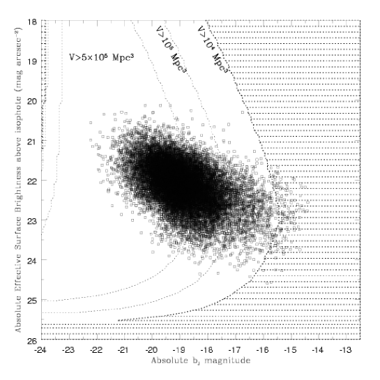
Figure 3: Galaxies from the 2dFGRS with redshifts, plotted in absolute magnitude and absolute effective surface brightness space. The shaded region denotes the regions where less than $10^{4}$ Mpc³ are surveyed and is based on visibility theory as described in Phillipps, Davies & Disney (1990). The 3 curves represent the volumes of $10^{4}$, $10^{5}$ and $5\times 10^{5}$ Mpc³.

Fig. 3 shows the upper panel of Fig. 2 with the axes converted to absolute parameter space using the conversions shown above. Naturally galaxies in different regions are seen over differing volumes, because of Malmquist bias, hence it is not yet valid to compare the relative numbers. However it is possible to define lines of constant volume as shown on Fig. 3 (dotted lines). These lines are derived from visibility theory (Phillipps, Davies & Disney 1990) and they delineate the region of the BBD plane where galaxies can be seen over various volumes. The shaded region shows the region where the volume is less than 10⁴ Mpc³ and hence where we are insensitive to galaxy densities of $<10^{-2}$galaxies/Mpc^-3mag^-1(mag arcsec^-2)^-1. The equations used to calculate the lines are laid out in Appendix B. We show a $V=5\times 10^{5}$Mpc³ line rather than $V=10^{6}$Mpc³ because the $z=0.12$ limit is at a volume less than $V=10^{6}$Mpc³. The parameters used in the visibility calculations are: $\mu_{lim}=24.67$ mag arcsec^-2; $\theta_{min}=7.2^{\prime\prime}$, $\theta_{max}=200.0^{\prime\prime}$, $m_{bright}=14.00$ mag; $m_{faint}=19.45$ mag; $z_{min}=0.015$; and $z_{max}=0.12$. The clear space between the data and the selection boundary at bright absolute magnitudes implies that although the 2dFGRS data set samples a sufficiently representative volume ($V>10,000$ Mpc³), galaxies only exist over a restricted region of this observed BBD. Fainter than $M=-16.5$ mags the volume is insufficient to sample populations with a space density of $10^{-2}$ Mpc^-3mag^-1(mag arcsec^-2)^-1 or less.

Fig. 4 shows the data of Fig. 3 binned into $\mu_{e}$ and $M$ intervals to produce the matrix $O(M,\mu)$ (see Eqn 4). The bins are $0.5$ mag$\times 0.5$ mag arcsec^-2 and start from $-24.0$mag and a central surface brightness of $19.0$mag arcsec^-2, effective surface brightness of $20.12$mag arcsec^-2. The total number of bins is 200 in a uniform $20\times 10$ array. Fig. 4 represents the observed distribution of galaxies and shows a strong peak close to the typical $M_{*}$ value seen in earlier surveys (see references listed in Table 1).

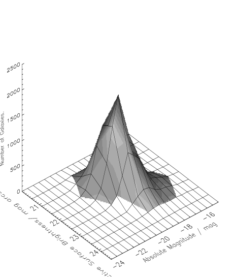
Figure 4: The observed distribution of the 2dFGRS data set mapped onto the BBD, prior to volume and incompleteness correction. The contour lines are set at 25, 100, 250, 500, 750, 1000, 1250, 1500 and 1750 galaxies per bin. The minimum number of galaxies in a bin is 25.

5.2 Deriving $I(M,\mu)$

Not all galaxies targeted by the 2dFGRS have a measured redshift. This may be due to lack of spectral features, selection biases or a misplaced/defunct fibre. One method to correct for these missing galaxies is to assume that they have the same observed BBD as those galaxies for which redshifts have been obtained. One can then simply scale up all bins by this known incompleteness.

However, from Fig. 2 and §1 & 3 we noted that the incompleteness is a function of both the apparent magnitude and the apparent surface brightness. There is no reliable way of converting these values to absolute values without redshifts and to obtain an incompleteness correction, $I(M,\mu)$, some assumption must be made. Here we assume that a galaxy of unknown redshift with apparent magnitude, $m$, and apparent effective surface brightness, $\mu_{e}$, has a range of possible BBD bins that can be statistically represented by the BBD distribution of galaxies with $m\pm\Delta m$ and $\mu_{e}\pm\Delta\mu_{e}$. The underlying assumption is that galaxies with and without redshifts with similar observed $m$ and $\mu$ have similar redshift distributions. I.e., the detectability of a galaxy is primarily dependent on its apparent magnitude and apparent surface brightness. [While these factors are obviously crucial one could also argue that additional factors, not incorporated here, such as the predominance of spectral features are also important such that the true probability distribution for the missing galaxies could be somewhat skewed from that derived in Fig. 5.]

Hence for each galaxy, without a redshift, we select those galaxies, with redshifts, within $0.1$mag and $0.1$mag arcsec^-2 and determine their collective observed BBD distribution. This is achieved using all 44796 galaxies in the SGP sample, as galaxies, without redshifts, are not limited to $z<0.12$. This distribution is then normalised to unity to generate a probability distribution for this galaxy. This is repeated for every galaxy without a redshift. Fig. 5, shows the probability distribution for a galaxy with $m=17.839$ and $\mu_{e}=22.314$. There are 317 galaxies with redshifts within $0.1$mag and $0.1$mag arcsec^-2 and combined they have a distribution ranging from $M=-15.44$ to $M=-21.76$ and $\mu_{e}=22.26$ to $\mu_{e}=21.06$.

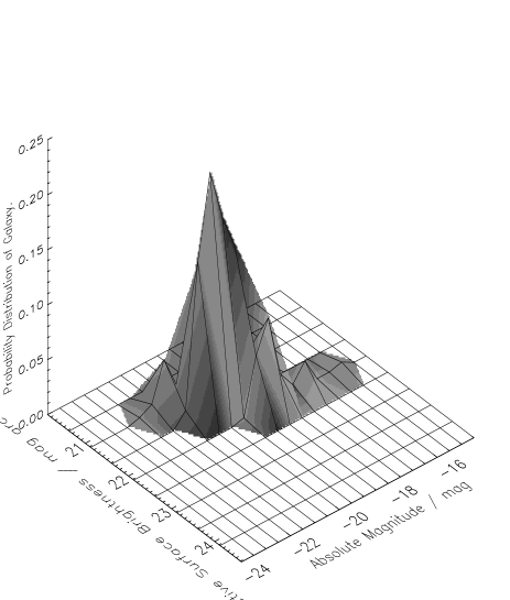
Figure 5: The BBD distribution of galaxies with $m=17.84\pm 0.1$ and $\mu_{e}^{app}=22.31\pm 0.1$. The contour lines are set at 0.01, 0.05, 0.10, 0.15 and 0.20 chance of the galaxy being in that bin.

To generate the matrix, $I(M,\mu)$, the probability distributions for each of the galaxies without redshifts, (normalised to unity) are summed together to give the total distribution of those galaxies without redshifts. However these galaxies could have the full range of redshifts that each galaxy can be detected over, not a range limited to $z=0.12$. Therefore the number distribution is weighted by the fraction of galaxies within each bin with $z<0.12$.

Fig. 6 shows $I(M,\mu)$ which should be compared to Fig. 4 ($O(M,\mu)$). The distribution of Fig 6 appears broader indicating that the missing galaxies are not random but that they are predominantly low luminosity, low surface brightness systems. This is illustrated in Fig. 7, which shows the ratio of $I(M,\mu)$ to $O(M,\mu)$ for the bins containing more than 25 galaxies with redshifts. From Fig. 7 we see that the trend is for the ratio to increase towards the low surface brightness regime. There is no significant trend in absolute magnitude. Finally we note that the although the incompleteness correction does increase the population in some bins by as much as 50% we shall see in §6 & 7 that the contribution from these additional systems towards the overall luminosity density is negligible.

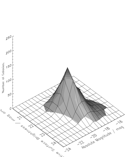
Figure 6: The bivariate number distribution of those galaxies without redshifts, i.e., $I(M,\mu)$. The contour lines are set at 10, 25, 50, 75, 100, 125 and 150 galaxies bin^-1.

Figure 7: The ratio of galaxies without redshifts to galaxies with redshifts. The contour lines are set at 0.01, 0.05, 0.10, 0.15, 0.20, 0.25, 0.30, 0.35, 0.40, 0.45 and 0.50.

5.3 Deriving $V(M,\mu)$

To convert the number of observed galaxies to number density per Mpc³ a Malmquist correction is required, i.e., $V(M,\mu)$. This matrix reflects the volumes over which each $M$, $\mu$ bin can be observed. One option is to use visibility theory as prescribed by Phillipps, Davies & Disney (1990) - and used to construct the constant volume line on Fig. 3. While visibility is clearly a step in the right direction, and preferable to applying a magnitude-only dependent correction, its limitation is that it assumes idealised galaxy profiles (i.e. it neglects the bulge component, seeing, star-galaxy separation and other complications). Ideally one would like to extract the volume information from the data itself and this is possible by using a $1/V_{\rm Max}$ type prescription, i.e., within each $O(M,\mu)$ bin, the maximum redshift at which a galaxy is seen is determined and the volume derived from this redshift. The advantages of using the data set rather than theory is that it naturally incorporates all redshift dependent selection biases. However the maximum redshift is susceptible to scattering from higher-visibility bins. An improved version is therefore to use the $90^{th}$ percentile redshift and to adjust $O(M,\mu)$ and $I(M,\mu)$ accordingly.

Although this requires rejecting 10% of the data it has two distinct advantages. Firstly it ensures that the redshift distribution in each bin has a sharp cutoff (as opposed to a distribution which peters out). Secondly it uses the entire dataset as opposed to the maximum redshift only. In the case where the $90^{th}$ percentile is not exact we take the galaxy nearest. Using these redshifts the volume can be calculated independently for each bin assuming an Einstein-de Sitter cosmology as follows:

$$V(M,\mu)=V_{z_{min}(M,\mu)}^{z_{90}(M,\mu)}$$ (19)

where,

$$V_{z_{min}(M,\mu)}^{z_{90}(M,\mu)}=\int^{z_{90}(M,\mu)}_{z_{min}(M,\mu)}\,\frac{\sigma\,c\,d_{l}^{2}}{H_{o}\,(1+z)^{3.5}}\,dz$$ (20)

and $\sigma$ is the solid angle in steradians on the sky. $d_{l}$ is the luminosity distance to the galaxy. $z_{min}$ is the minimum distance over which a galaxy can be detected. $z_{min}$ is calculated from visibility theory (Phillipps, Davies & Disney 1990, see also Appendix B) adopting values for the maximum magnitude and maximum size of $m_{B}=14.00$ mag and $\theta=200^{\prime\prime}$ respectively.

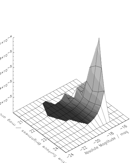
Figure 8: Plot of 1/volume in each bin. The contour lines are set at $1.0\times 10^{-7}$, $1.0\times 10^{-6}$, $2.0\times 10^{-6}$, $1.0\times 10^{-5}$, $2.0\times 10^{-5}$, $4.0\times 10^{-5}$, $6.0\times 10^{-5}$, $8.0\times 10^{-5}$ and $1.0\times 10^{-4}$ h^-3 Mpc^-3.

Fig. 8 shows the matrix $\frac{1}{V(M,\mu)}$. Note that squares containing fewer than 25 galaxies are not shaded. This matrix is flat-bottomed due to the cutoff at $z=0.12$. Fig. 8 shows a strong dependency upon magnitude (i.e. classical Malmquist bias as expected) and also upon surface brightness. This surface brightness dependency is particularly strong near the $10^{4}$ Mpc³ volume limit, as the data becomes sparse. Inside this volume limit the contour lines generally mimic the curve of the visibility-derived volume boundary. This suggests that visibility theory provides a good description of the combined volume dependency. The sharp cutoff along the high surface brightness edge may be real but could also be a manifestation of the complex star-galaxy separation algorithm (see Maddox 1990a). Given that a galaxy seen over a larger distance appears more compact and that local dwarfs have smaller scale lengths than giants (cf. Mateo 1998), this seems reasonable. We will investigate this further through high-resolution imaging.

The main point to take away from Fig. 8 is that the visibility surface of the 2dFGRS input catalogue is complex and dependent on both $M$ and $\mu_{e}$ (although predominantly $M$). Any methodology which ignores surface brightness information and implements a volume-bias correction in luminosity only, is implicitly assuming uniform visibility in surface brightness. The 2dFGRS data clearly show that this is not the case.

5.4 Clustering

Structure is seen on the largest measurable scales (e.g. de Lapparent, Gellar & Huchra 1986). To determine whether the effects of clustering are significant we constructed a radial density profile, as shown in Fig. 9. This was derived from those bins for which more than 100 galaxies are seen over the whole range from $0.015<z<0.12$ (i.e. $-19.75<M<-18.75$ and $21.1<\mu_{e}<22.6$). Those galaxies which are brighter cannot be seen at $z<0.015$ due to the bright magnitude cut at $m=14.00$ and would therefore bias the number density towards the bright end. For these high-visibility galaxies we calculated their number-density ($\phi$) in equal volume intervals of $5.0\,\times 10^{3}$ Mpc³, from $z=0.0185$ to $z=0.12$. Fig. 9 shows that clustering is severe with what appears to be a large local void around $z=0.04$ and walls at $z=0.06$ and $z=0.11$. The ESO Slice Project (ESP) survey (Zucca et al. 1997) whose line-of-sight (RA $\sim 00$h, $\delta\sim-40$) is just outside the 2dF SGP region, measures an under-density at $\leq 140h^{-1}$Mpc ($z\approx 0.045$) and an over-density at $z\approx 0.1$. The structure that they see closely resembles the structure that we see. A reliable measure of the BBD needs to correct for this clustering-bias. Here we adopt a strategy which implicitly assumes, firstly, that clustering is independent of either $M$ or $\mu$, and secondly, that evolutionary processes to z = 0.12 are negligible.

Figure 9: The clustering map. This shows the number density of giant galaxies ($-19.75<M<-18.75$ and $21.1<\mu_{e}<22.6$ as a function of redshift. The points are spaced equally in volume at intervals of 5000 h³ Mpc³ starting at 10000 h³ Mpc³.

On the basis of these caveats we constructed a weighting matrix, $W(M,\mu)$. This was determined from the high-visibility galaxies by taking the ratio of the number-density of high-visibility galaxies over the full redshift range divided by the number-density of high-visibility galaxies over the redshift range of each bin, i.e.:

$$W(M,\mu)=\frac{\bar{\phi}(High-vis)^{z=0.12}_{z=0.015}}{\phi(High-vis)^{zmax(M,\mu)}_{zmin(M,\mu)}}$$ (21)

This weighting matrix is shown in Fig. 10. The implication is that the number-density of low-luminosity systems will be amplified by almost a factor of 1.5, to correct for the apparent presence of a large local void along the SGP region - indicated by the vertical ridge at $M=-17$ on Fig. 10. Once again this implicitly assumes that the clustering of dwarf and giant systems is correlated.

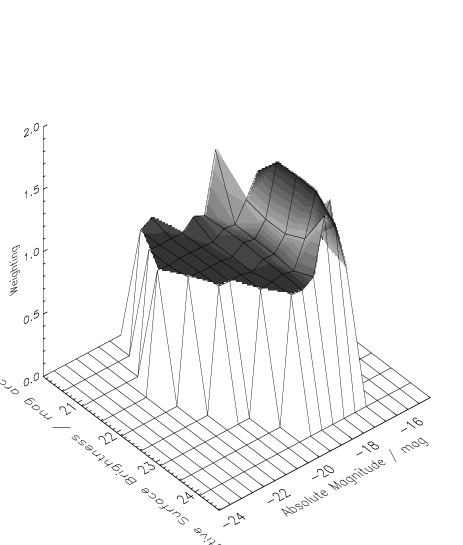
Figure 10: The Weighting Map. The contours are at 0.8, 0.9, 1.0, 1.1, 1.2, 1.3, 1.4 and 1.5.

6 The 2dFGRS BBD

Finally we can combine the four matrices, $O(M,\mu)$, $I(M,\mu)$, $V(M,\mu)$ and $W(M,\mu)$ (see Eqn 4), to generate the 2dFGRS bivariate brightness distribution, as shown in Fig. 11. This depicts the underlying local galaxy number-density distribution inclusive of surface brightness selection effects. Only those bins which are based upon 25 or more galaxies are shown. Note that by summing the BBD along the surface brightness axis one recovers the luminosity distribution of galaxies. By summing along the magnitude axis one obtains the surface brightness distribution of galaxies (see §8).

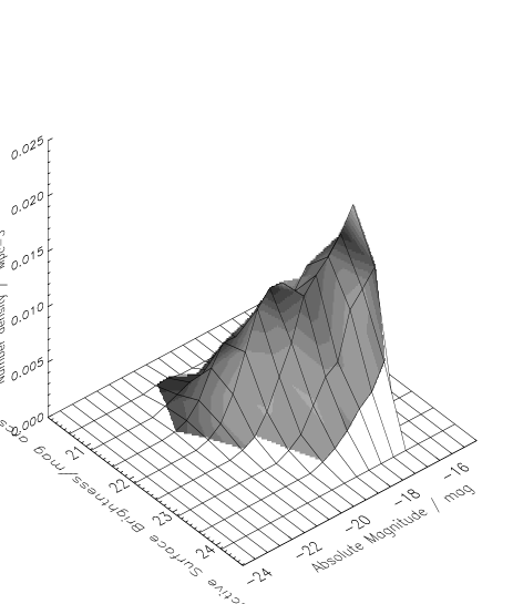
Figure 11: The 2dFGRS Bivariate Brightness Distribution.The contour lines are set at $1.0\times 10^{-7}$, $1.0\times 10^{-3}$, $2.5\times 10^{-3}$, $5.0\times 10^{-3}$, $7.5\times 10^{-3}$, $1.0\times 10^{-2}$, $1.25\times 10^{-2}$, $1.5\times 10^{-2}$, $1.75\times 10^{-2}$, $2.0\times 10^{-2}$, and $2.25\times 10^{-2}$ galaxies Mpc^-3 bin^-1. The thick lines represent the selection boundaries calculated from visibility theory.

Figure 12: The errors in the BBD. The contour lines are set at $1.0\times 10^{-7}$, $1.0\times 10^{-4}$, $5.0\times 10^{-4}$, $1.0\times 10^{-3}$, $1.5\times 10^{-3}$, $2.0\times 10^{-3}$, $2.5\times 10^{-3}$, $3.0\times 10^{-3}$, $3.5\times 10^{-3}$ and $4.0\times 10^{-3}$ galaxies Mpc^-3 bin^-1.

Fig. 12 shows the errors in the BBD. These were initially determined via Monte-Carlo simulations, assuming a Gaussian error distribution of $\pm 0.2$ mag, in the APM magnitudes. This showed that the errors were proportional to $\sqrt{(1/N)}$, and since $\sqrt{(1/N)}$ is much faster to calculate, this is the result that is used throughout the calculations. These errors were then combined in quadrature with the additional error in the volume estimate, assuming Poisson statistics. The total error is given by:

$$\sigma_{\phi}=\sqrt{(\frac{1}{N_{tot}(M,\mu)})+(\frac{1}{N_{z}(M,\mu)})}$$ (22)

The errors become significant ($>$ 20%), when $M>-16$ and around the boundaries of the BBD shown in Fig. 11. The data and associated errors are tabulated in Table 2. From Figs 11 & 12 we note the following:

6.1 A luminosity-surface brightness relation

The BBD shows evidence of a luminosity-surface brightness relation similar to that seen in Virgo, ($M_{B}\propto 1.6\mu_{o}$, Binggeli 1993), in the Hubble Deep Field, ($M_{F450W}\propto 1.5\mu_{e}$, Driver 1999) and in Sdm galaxies ($M_{B}\propto 2.02\pm 0.16\mu_{e}$ de Jong & Lacey 2000). A formal fit to the 2dFGRS data yields $M_{B}\propto(2.4\pm^{1.5}_{0.5})\mu_{e}$. While confirming the general trend this result appears significantly steeper than the Virgo and HDF results. Both the Virgo and HDF results are based on lower luminosity systems hence this might be indicative of a second order dependency of the relation upon luminosity. Alternatively it may reflect slight differences in the data/analysis as neither the Virgo nor HDF data include isophotal corrections whereas the 2dFGRS data is more susceptible to atmospheric seeing. The gradient is slightly steeper than the de Jong & Lacey result, but is well within the errors.

The presence of a luminosity-surface brightness relation highlights concerns over the completeness of galaxy surveys, as surveys with bright isophotal limits will preferentially exclude dwarf systems leading to an underestimate of their space-densities and variations such as those seen in Fig. 1.

The confirmation of this luminosity-surface brightness relation within such an extensive dataset is an important step forward and any credible model of galaxy formation must now be required to reproduce this relation.

6.2 A Dearth of Luminous Low surface brightness galaxies

Within each magnitude interval there appears to be a preferred range in surface brightness over which galaxies may exist. While the high-surface brightness limit may be due, in part or whole, to star-galaxy separation and/or fibre-positioning accuracy the low surface brightness limit appears real. This cannot be a selection limit as one requires a mechanism which hides luminous LSBGs yet allows dwarf galaxies of similar surface brightness to be detected within the same volume. The implications are that these galaxy types (luminous-LSBGs) are rare with densities less than $10^{-4}$ galaxies Mpc^-3. This result is important as it directly addresses the issues raised in the introduction and implies that existing surveys have not missed large populations of luminous low surface brightness galaxies. Perhaps more importantly it confirms that the 2dFGRS is complete for giant galaxies and that the postulate that the Universe might be dominated by luminous LSBGs (Disney 1976) is ruled out.

One caveat however is that luminous-LSBGs could be masquerading as dwarfs. For example consider the case of Malin 1 (Bothun et al. 1987) which has a huge extended disk ($55$ kpc scale-length) of very low surface brightness ($\mu_{o}=26.5$). This system is actually readily detectable because of its high surface brightness active core, however within the 2dFGRS limits it would have been miss-classified as a dwarf system with $M=-17.9$, $\mu_{e}=21.8$. Hence Figs 11 & 12 rule out luminous disk systems only. To determine whether objects such as Malin 1 are hidden amongst the dwarf population will require either ultra-deep CCD imaging or cross-correlation with HI-surveys which would exhibit very high HI mass-to-light ratios for such systems.

6.3 The rising dwarf population

The galaxy population shows a steady increase in number-density with decreasing luminosity. This continues to the survey limits at $M=-16$, whereupon the volume limit and surface brightness selection effects impinge upon our sample. The expectation is that the distribution continues to rise and hence the location of the peak in the number-density distribution remains unknown. However we do note that the increase seen within our selection limits is insufficient for the dwarf population to dominate the luminosity-density as shown in the next section.

Perhaps more surprising is the lack of sub-structure indicating either a continuity between the giant and dwarf populations or that any sub-structure is erased by the random errors. The former case is strongly indicative of a hierarchical merger scenario for galaxy formation which one expects to lead towards a smooth number-density distribution between the dwarf and giant systems (White & Rees, 1978). This is contrary to the change in the luminosity distribution of galaxies seen in cluster environments (e.g. Smith, Driver, & Phillipps 1997). In a later paper we intend to explore the dependency of the BBD upon environment.

7 The value of $j_{B}$ and $\Omega_{M}$

The luminosity density matrix, $j(M,\mu)$ is constructed from $L\,\Phi(M,\mu)$ in units of $L_{\odot}$Mpc^-3 and is shown as Fig. 13. The distribution is strongly peaked close to the conventional $M_{*}$ parameter derived in previous surveys (see Table 1). The peak lies at $M=-19.5$ mag and $\mu_{e}=22.12$ mag arcsec^-2. The final value obtained is $j_{B}=(2.49\pm 0.20)\times 10^{8}h_{100}L_{\odot}$Mpc^-3. The sharp peak sits firmly in the centre of our observable region of the 2dFGRS BBD and drops rapidly off on all sides towards the 2dFGRS BBD boundaries. This implies that while the 2dFGRS does not survey the entire parameter space of the known BBD it does effectively contain the full galaxy contribution to the local luminosity density. Redoing the calculations using galaxies with redshifts also results in $j_{B}=(2.49\pm 0.20)\times 10^{8}h_{100}L_{\odot}$Mpc^-3. This demonstrates that there is no dependency of the results upon the assumption made for the distribution of galaxies without redshifts.

We note that $j$ derived via a direct $\frac{1}{V_{max}}$ estimate, without any surface brightness or clustering corrections, (Eqn 1) gives a value of $j=1.82\pm 0.07\times 10^{8}h_{100}L_{\odot}$Mpc^-3. Including the isophotal magnitude correction only leads to a value of $j=2.28\pm 0.09\times 10^{8}h_{100}L_{\odot}$Mpc^-3. Hence a more detailed analysis leads to a 36.8% increase in $j$, of this 36.8%, 25.3% is due to the isophotal correction, 10.4% is due to the Malmquist bias correction and 1.1% is due to the clustering correction.

The final value agrees well with that obtained from the recent ESO Slice Project (Zucca et al. 1997). The method that they used corrects for clustering, but not surface brightness — although their photometry is based on aperture rather than isophotal magnitudes. However it is worth pointing out that $j$ is sensitive to the exact value of $\mu_{lim}$. The quoted error in $\mu_{lim}$ is $\pm 0.3$ (for plate-to-plate variations, Metcalfe et al 1995; Pimblett et al 2000). Table 3 shows a summary of results when repeating the entire analysis using the upper and lower error limits. It therefore seems likely that a combination of surface brightness biases and large scale structure can indeed lead to the type of variations seen in Table 1.

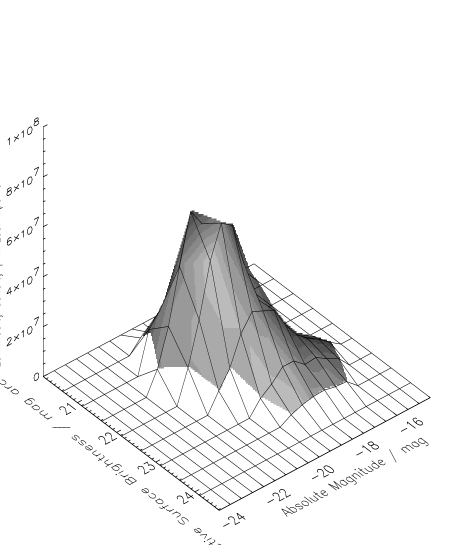
Figure 13: Plot of the Luminosity Density Distribution. The contour lines are set at 100, $1.0\times 10^{6}$, $5.0\times 10^{6}$, $1.0\times 10^{7}$, $2.0\times 10^{7}$, $3.0\times 10^{7}$, $4.0\times 10^{7}$, $5.0\times 10^{7}$, and $6.0\times 10^{7}$L_⊙ Mpc^-3 bin^-1.

Finally following the method of Carlberg, Yee & Ellingson (1997) we can obtain a crude ball-park figure for the total local mass density by adopting a universal mass-to-light ratio based on that observed in clusters. While this method neglects biasing (White, Tully & Davis, 1988) it does provide a useful crude upper limit to the mass density. From Carlberg et al. (1997) we find: $\frac{{\cal M}_{Dyn}}{L_{R}}=289\pm 50h_{100}\frac{{\cal M}_{\odot}}{L_{\odot}}$. Assuming a mean colour of $(B-R)=1.1$ and a solar colour index of 1.17 this converts to: $\frac{{\cal M}_{Dyn}}{L_{B}}=271\pm 47h_{100}\frac{{\cal M}_{\odot}}{L_{\odot}}$. Multiplying the luminosity density by the mass-to-light ratio yields a value for the local mass-density of $\Omega_{M}\approx 0.24$. We note that this is consistent with the current constraints from the combination of Sn Ia results with the recent Boomerang and Maxima-1 results (Balbi et al. 2000; de Bernardis et al. 2000).

8 Comparisons with other surveys

As this work represents the first detailed measure of the field BBD there is no previous work with which to compare. However as mentioned earlier it is trivial to convert the BBD into either a luminosity distribution and/or a surface brightness distribution both of which have been determined by numerous groups. This is achieved by summing across either luminosity or surface brightness intervals. For those bins containing fewer than 25 galaxies for which a volume- and clustering- bias correction were not obtained we use the volume-bias correction from the nearest bin with 25 or more galaxies. This will lead to a slight underestimate in the number-densities, however as the number-density peak is well defined this effect is negligible.

8.1 The luminosity distribution

Fig. 14 shows a compendium of luminosity function measures (see Table 1 and Fig. 1). Superimposed on the previous Schechter function fits (dotted lines) are the results from the 2dFGRS. Three results are shown, the luminosity distribution neglecting surface brightness and clustering (short dashed line), the luminosity distribution inclusive of surface brightness corrections (long dashed line) and finally the luminosity distribution inclusive of surface brightness and clustering corrections (solid line). The inset shows the $2\sigma\,\chi^{2}$ error eclipse for the latter case, yielding Schechter function parameters of $M_{*}=-19.75\pm 0.05,\alpha=-1.09\pm 0.03$ and $\phi_{*}=0.0202\pm 0.0002$ in close agreement with the ESO Slice Project (ESP, see Table 1).

Comparing the 2dFGRS result with other surveys suggests that the main effect of the surface brightness correction is to shift $M_{*}$ brightwards by the mean isophotal correction of 0.33 mag and to increase the number density by a factor of 1.2. The clustering correction has little effect at bright magnitudes, almost by definition, but significantly amplifies the dwarf population. This is a direct consequence of an apparent local void at z=0.04 along the full range of the 2dF SGP region.

We note that the combination of these two corrections mimics closely the discrepancies between various Schechter function fits. For example the shallower SSRS2, APM and Durham/UKST surveys are biased at all magnitudes by the apparent local void while the deeper ESP and Autofib surveys (which employ clustering independent methods) probe beyond the void. Similarly because of the luminosity-surface brightness relation those surveys which probe to lower surface brightnesses will find a higher dwarf-to-giant ratio.

The shaded region shows the point at which our data starts to become highly uncertain because of the small volume surveyed ($V<10,000$ Mpc³). As this is the first statistically significant investigation into the bivariate brightness distribution we can conclude that as yet no survey contains any direct census of the space density of $M_{B}>-16.0$ mag galaxies.

Figure 14: The solid line shows the final luminosity function, with all corrections taken into account. The long dashed line shows the luminosity function with surface brightness corrections only, and the short dashed line shows the luminosity function ignoring surface brightness and clustering corrections. Also shown, as dotted lines, are the luminosity functions from Fig. 1. The shaded region denotes the limit of reliability based on visibility theory.

8.2 The surface brightness distribution

There have been a few Surface Brightness Functions published over the years. The first was the Freeman (1970) result, which showed a Gaussian distribution with $\bar{\mu}=21.65$ and $\sigma_{\mu}=0.3$. Since then, however, many galaxies have been found at greater than 10$\sigma$ from the mean. The probability of a galaxy occurring at 10$\sigma$ or greater is $\approx 1\times 10^{-20}$. The total number of galaxies in the universe is in the range of $10^{11}$ — $10^{12}$, so the Freeman SBF must be underestimating the LSBGs. The distribution seen by Freeman is almost certainly due to the relatively bright isophotal detection threshold that the observations were taken at, around 22 - 23 mag arcsec^-2. A more recent measure of the SBF comes from O’Neil & Bothun (2000) who also show a compendium of results from other groups. The O’Neil & Bothun data in contrast to the Freeman result shows a flat distribution over the range $22<\mu_{o}<25$ albeit with substantial scatter. Fig. 15 reproduces Fig. 1. of O’Neil & Bothun but now includes the final 2dFGRS results. In order to compare our results directly with the O’Neil & Bothun data we assumed a mean bulge-to-total ratio of 0.4 (see Kent 1985) resulting in a uniform offset of $0.55$ mag arcsec^-2.

The 2dFGRS data is substantially broader than the Freeman distribution and appears to agree well with the compendium of data summarised in O’Neil & Bothun (2000). From visibility theory (see Fig. 3) we are complete (i.e. the volume observed is greater than $10^{4}$ Mpc³ and therefore statistically representative) in central surface brightness from $18.0<\mu_{o}<23$ for $M<-16$. Assuming that the luminosity-surface brightness relation continues as reported in Driver (1999) and Driver & Cross (2000) the expectation is that the surface brightness distribution will steepen as galaxies with lower luminosities are included.

Figure 15: The solid line shows the final surface brightness function, with all the surface brightness and clustering corrections. The points are offset towards the low surface brightness direction by 0.55 mag to crudely correct for the bulge. Also shown is the O’Neil & Bothun (2000) data, as crosses with error bars. The shaded region is where the visibility line shown in the previous diagrams starts to cross the data and so the data is no longer completely reliable.

9 Conclusions

We have introduced the bivariate brightness distribution as a means by which the effect of surface brightness selection biases in large galaxy catalogues can be investigated. By correcting for the light below the isophote and including a surface brightness dependent Malmquist correction we find that the measurement of the luminosity density is increased by $\sim 37$% over the traditional $\frac{1}{V_{max}}$ method of evaluation. The majority (25%) of this increase comes from the isophotal correction with 10% due to incorporating a surface brightness dependent Malmquist correction and 1% due to the clustering correction.

We have shown that our isophotal correction is suitable for all galaxy types and that isophotal magnitudes without correction severely underestimate the magnitudes for specific galaxy types. We also note that the redshift incompleteness suggests that predominantly low surface brightness galaxies are being missed however we also show that these systems are predominantly low luminosity and hence contribute little to the overall luminosity density. This is in part due to the high completeness of the 2dFGRS ($\sim 91$ %).

We rule out the possibility of the 2dFGRS missing a significant population of luminous giant galaxies down to $\mu_{e}=24.5$ mag arcsec^-2 (or $\mu_{o}=23.5$ mag arcsec^-2) and note that the contribution at surface brightness limits below $\mu_{e}=23$ mag arcsec^-2 is small and declining. Dwarf galaxies greatly outnumber the giants and the peak in the number density occurs at the low luminosity selection boundary. The implication is that the most numerous galaxy type lies at $M>-16.0$ mag. The galaxy population as a whole follows a luminosity-surface brightness relation ($M\propto(2.4\pm^{1.5}_{0.5})\mu_{e}$), similar but slightly steeper, to that seen in Virgo, in the Hubble Deep Field and in SdM galaxies. This relation provides an additional constraint which galaxy formation models must satisfy.

We conclude that our measure of the galaxy contribution to the luminosity density is robust and dominated by conventional giant galaxies with only a small ($<10$%) contribution from dwarf ($M>-17.5$ mag) and/or low surface brightness giants ($\mu_{e}>23$ mag arcsec^-2) within the selection boundaries($-24<M_{B}<-15.5$ mag, $18.0<\mu_{e}<24.5$ mag arcsec^-2). However we cannot rule out the possibility of a contribution from an independent population outside of our optical selection boundaries.

Our measurement of the luminosity density is $j=2.49\pm 0.20\times 10^{8}h_{100}$L_⊙Mpc^-3 and using a typical cluster mass-to-light ratio leads to an estimate of the matter density of order $\Omega_{M}\sim 0.24$ in agreement with more robust measures.

Finally we note that the bivariate brightness distribution offers a means of studying the galaxy population and luminosity-density as a function of environment and epoch fully inclusive of surface brightness selection biases. Future extensions to this work will include the measurement of BBDs and “population peaks” for individual spectral/morphological types, and as a function of redshift and environment. This step forward has only become possible because of the recent availability of large redshift survey databases such as that provided by the 2dFGRS.

References

Babul, A., Rees, M., 1992, MNRAS, 255, 346

Babul, A., Ferguson, H.C., 1996, ApJ, 458, 100

Balbi A., Ade P., Bock J., Borrill J., Boscaleri A., de Bernardis P., Ferreira P.G., Hanany S., Hristov V.V., Jaffe A.H., Lee A.T., Oh S., Pascale E., Rabii B., Richards P.L., Smoot G.F., Stompor R., Winant C.D., Wu J.H.P. 2000, ApJL in press (astro-ph 0005124)

Beijersbergen, M., de Blok, W.J.G., van der Hulst, J.M. 1999, A&A, 351, 903

Binggeli B., 1993 in ESO/OHP Workshop on Dwarf Galaxies, Eds Meylan G., & Prugniel, P., (Publ: ESO, Garching), 13

Binggeli, B., Sandage, A., Tammann, G.A., 1988, ARA&A, 26, 509

Bothun, G.D., Impey, C.D., Malin, D.F., Mould, J.R. 1987, AJ, 94, 23

Boyce, P.J., Phillipps, S., 1995, A&A, 296, 26

Bristow, P.D., Phillipps, S., 1994, MNRAS, 267, 13

Carlberg, R.G., Yee, H.K.C., Ellingson, E., Abraham, R. Gravel, P., Morris, S. Pritchet, C.J. 1996, ApJ, 462, 32

Carlberg, R.G., Yee, H.K.C., Ellingson, E. 1997, ApJ, 478, 462

Colless, M. 1999, Phil.Trans.RSoc., 357, 105

Dalcanton, J.J., Spergel, D.N., Gunn, J.E., Schmidt, M., Schneider, D.P., 1997, AJ, 114, 635

Dalcanton, J.J., 1998, ApJ, 495, 251

de Bernardis, P., Ade P.A.R., Bock J.J., Bond J.R., Borrill J., Boscaleri A., Coble K., Crill B.P., De Gasperis G., Farese P.C., Ferreira P.G., Ganga K., Giacometti M., Hivon E., Hristov V.V., Iacoangeli A., Jaffe A.H., Lange A.E., Martinis L., Masi S., Mason P., Mauskopf P.D., Melchiorri A., Miglio L., Montroy T., Netterfield C.B., Pascale E., Piacentini F., Pogosyan D., Prunet S., Rao S., Romeo G., Ruhl J.E., Scaramuzzi F., Sforna D., Vittorio N. 2000, Nature, 404, 955

de Jong R. & Lacey C. 2000. Accepted for publication in ApJ

de Lapparent, V., Gellar, M.J., Huchra, J.P. 1986, ApJ, 304, 585

de Vaucouleurs, G. 1948, Ann. Astrophys., 11, 247

Disney, M. 1976, Nature, 263, 573

Driver, S.P., Phillips, S., Davies, J.I., Morgan, I., Disney, M.J. 1994, MNRAS, 266, 155

Driver, S.P., Windhorst, R.A., Griffiths, R.E. 1995, ApJ, 453, 48

Driver, S.P., Couch, W.J., Phillipps, S., 1998, MNRAS, 301, 369

Driver, S.P. 1999, ApJL, 526, 69

Driver, S.P., Cross N.J.G. 2000, in Mapping the Hidden Universe, Eds R. Kraan-Korteweg, P. Henning & H. Andernach (Publ: Kluwer), (astro-ph 0004201)

Efstathiou, G., Ellis, R., Peterson, B. 1988, MNRAS, 232, 431

Ellis, R.S., Colless, M., Broadhurst, T., Heyl, J., Glazebrook, K. 1996, MNRAS, 280, 235

Ellis, R.S., 1997, ARA&A, 35, 389

Felten, J.E., 1985, Com Ap, 11, 53

Ferguson, H.C., Binggeli, B. 1994, A&ARv, 6, 67

Fernández-Soto A., Lanzetta K., Yahil A., 1998, ApJ, 513, 34

Folkes, S., Ronen, S., Price, I., Lahav, O., Colless, M., Maddox, S., Deeley, K., Glazebrook, K., Bland-Hawthorn, J., Cannon, R., Cole, S., Collins, C., Couch, W., Driver, S., Dalton, G., Efstathiou, G., Ellis, R., Frenk, C., Kaiser, N., Lewis, I., Lumsden, S., Peacock, J., Peterson, B., Sutherland, W., Taylor, K. 1999, MNRAS, 308, 459

Freeman, K. 1970, ApJ, 160, 811

Fukugita M., Hogan C.J., Peebles P.J.E., 1998, ApJ, 503, 518

Gaztanaga, E., Dalton, G.B. 2000, MNRAS, 312, 417

Impey, C., Bothun, G. 1997, ARA&A, 35, 267

Jerjen, H. Binggeli, B. 1997, ’The Nature of Elliptical Galaxies’, Eds. M. Arnaboldi, G.S. Da Costa & P. Saha, (Canberra: Mt Stromlo Observatory) p. 239

Kent, S.M. 1985, ApJS, 59, 115

Koo D.C., Kron R.G., 1992, ARA&A, 30, 613

Lilly, S. J., Le Fevre, O., Hammer, F., Crampton, D. 1996, ApJ, 460, 1

Lin, H., Kirshner, R., Shectman, S., Landy, S., Oemler, A., Tucker, D., Schechter, P. 1996, ApJ, 464, 60

Loveday, J., Peterson B. A., Efstathiou, G., Maddox, S. J. 1992, ApJ, 390, 338

Loveday, J., 1997, ApJ, 489, 29

Loveday, J., 2000, MNRAS, 312, 557

Madau, P., Della Valle, M., Panagia, N. 1998, ApJ, 498, 106

Maddox, S.J., Sutherland, W.J., Efstathiou, G., Loveday, J. 1990, MNRAS, 243, 692

Maddox, S.J., Efstathiou, G., Sutherland, W.J. 1990, MNRAS, 246, 433

Margon, B. 1999, Phil.Trans.RSoc., 357, 105

Marzke, R., Huchra, J., Geller M. 1994, ApJ, 428, 43

Marzke, R., Da Costa, N., Pelligrini, P., Willmer, C., Geller M. 1998, ApJ, 503, 617

Mateo, M.L. 1998, ARA&A, 36, 435

McGaugh, S.S., 1992, PhD Thesis, Univ. Michigan

McGaugh, S.S., 1996, MNRAS, 280, 337

Metcalfe, N. , Fong, R. Shanks T. 1995, MNRAS, 274, 769

Minchin, R.F. 1999, PASA, 16, 12

O’Neil, K,. Bothun G.D., 2000, ApJ, 529, 811

Persic, M., Salucci, P., 1992, MNRAS, 258, 14pp

Petrosian, V. 1998, ApJ, 507, 1

Phillipps, S., Disney, M. 1986, MNRAS, 221, 1039

Phillipps, S., Davies, J., Disney, M. 1990, MNRAS, 242, 235

Phillipps, S., Driver, S.P., 1995, MNRAS, 274, 832

Phillipps, S., Driver, S.P., Couch, W.J., Smith, R.M., 1998, ApJL, 498, 119

Pimbblet, K., et al. 2000, (submitted).

Ratcliffe, A., Shanks, T., Parker, Q., Fong R. 1998, MNRAS, 293, 197

Sandage, A., Tammann, G.A. 1981, ’A Revised Shapley- Ames Catalog of Bright Galaxies.’ (Washington DC: Carnegie Institute of Washington).

Schechter, P. 1976, ApJ, 203, 297

Shanks, T. 1990, Proc. IAU Symp. 139 on Extragalactic Background Radiation, Eds S.C. Bowyer, C. Leinert, (Publ:Kluwer), 139, 269

Sodre L(Jr), Lahav O., 1993, MNRAS, 260, 285

Smith, R.M., Driver, S.P., Phillipps, S. 1997, MNRAS, 287, 415

Smoker, J.V., Axon, D.J., Davies, R.D. 1999, A&A, 341, 725

Sprayberry D., Impey, C., Irwin, M., 1996, ApJ, 463, 535

Taylor, K., Cannon, R.D., Parker, Q., 1998, in IAU symp. 179, Eds.B.J.,McLean., D.A.Golembek, J.J.E.Haynes & H.E.Payne, (Publ:Kluwer), p 135

Trentham, N., 1998, MNRAS, 294, 193

van den Bergh, S., 1998, ’Galaxy Morphology and Classification.’ (Publ. CUP)

Williams R.E., et al. 1996, AJ, 112, 1335

Willmer, C.N.A., 1997, AJ, 114, 898

White, S.D.M. & Rees, M.J. 1978, MNRAS, 183, 341

White, S.D.M., Tully, B. & Davis, M. 1988, ApJ, 333, L45.

Zucca, E., Zamorani, G., Vettolani, G., Cappi, A., Merighi, R., Mignoli, M., Stirpe, G.M., Macgillivray, H., Collins, C. and Balkowski, C., Cayatte, V., Maurogordato, S., Proust, D. and Chincarini, G., Guzzo, L., Maccagni, D., Scaramella, R., Blanchard, A., Ramella, M. 1997, A&A, 326, 477

Appendix A Testing the isophotal corrections

It is possible to model several different types of galaxy and compare the isophotal magnitude and the total magnitude as calculated in §4 with the “true” magnitude. The models are simple, assuming a face on circular galaxy, composed of a bulge with a de Vaucouleurs $r^{\frac{1}{4}}$ law (de Vaucouleurs 1948) and a disk with an exponential profile (see Eqn. 8).

$$\mu_{bulge}=\mu_{e}+1.40+8.325[(r/r_{e})^{1/4}-1]$$ (23)

where $r_{e}$ is the half-light radius of the bulge, $\mu_{e}$ is the effective surface brightness of the bulge. Here we define it as the mean surface brightness within $r_{e}$. However, it is more useful to define galaxies in terms of their luminosities and bulge-to-disk ratios than their effective radii or disk scale-lengths.

The magnitude of a galaxy and the bulge-disk ratio can be found in terms of the above parameters, by:

$$\begin{split}&M=-2.5\log_{10}[10^{-0.4B}+10^{-0.4D}]\\ &B/T=\frac{B}{B+D}=\frac{1}{1+1/(\frac{B}{D})}\\ &B=\mu_{e}+1.40-2.5\log_{10}[7.22\pi\,r_{e}^{2}]\\ &D=\mu_{o}-2.5\log_{10}[\pi\,\alpha^{2}]\\ \end{split}$$ (24)

where $B$ is the magnitude of the bulge and $D$ is the magnitude of the disk. $B/T$ is the bulge-to-total ratio. Given the parameters $M$, $B/T$, $\mu_{e}$ and $\mu_{o}$, a galaxy’s light profile is fully defined.

To calculate the difference between the total and the isophotal magnitude it is necessary to find the fraction of light lost below the isophote. Since the intrinsic detection isophote varies with the redshift, this difference will be a function of redshift. For a variety of redshifts from $z=0.001$ to $z=0.201$, the fraction of light under the isophote was calculated, by first converting the above magnitudes to apparent magnitudes, the intrinsic surface brightnesses to apparent surface brightnesses and then calculating the scale-lengths as above. The conversions from absolute to apparent properties are given in Eqn. 17 and Eqn. 18.

Using $\mu_{lim}=24.67$mag arcsec^-2, the isophotal radii of the disk and bulge are calculated.

$$\begin{split}&r_{iso,d}=(\frac{\mu_{lim}-\mu_{o}}{1.086})\,\alpha\\ &r_{iso,b}=(\frac{\mu_{lim}-(\mu_{e}+1.40)}{8.325}+1)^{4}\,r_{e}\\ \end{split}$$ (25)

The fraction of light above the isophote is then calculated using the equation below.

$$f=1-\sum_{n=0}^{2\beta-1}\frac{1}{n!}g^{n}\,e^{-g}$$ (26)

where $\beta$ is the de Vaucouleur’s parameter, which is 1 for a disk and 4 for a bulge. $g=7.67(\frac{r}{r_{e}})^{1/4}$ in bulges and $g=\frac{r}{\alpha}$ in disks. The isophotal magnitude and isophotal radius of the galaxy can now be calculated.

$$\begin{split}&m_{iso,b}=m_{b}-2.5\log_{10}\,f_{b}\\ &m_{iso,d}=m_{d}-2.5\log_{10}\,f_{d}\\ &m_{iso}=-2.5\log_{10}[10^{-0.4m_{iso,b}}+10^{-0.4m_{iso,d}}]\\ &r_{iso}=\rm{max}(r_{iso,b},r_{iso,d})\\ \end{split}$$ (27)

Now that the isophotal magnitude, $m_{ISO}$, has been found it is possible to convert it back to an absolute magnitude, $M_{ISO}$. The isophotal magnitude and radius are fed now back through the equations in §4 and a value of $m^{corr}$ is calculated. This is converted to an absolute magnitude and Table 4 shows a comparison of $M_{true}$, $M_{iso}$ and $M_{corr}$ at $z=0.12$ for the main Hubble Type galaxies and low surface brightness galaxies. The properties of the LSBGs ($B/T$, $\mu_{e}$ and $\mu_{o}$) come from averaging the B-band data in Beijersbergen, de Blok & van der Hulst (1999), the values of $B/T$ for S0, Sa, Sb and Sc galaxies are taken from Kent (1985). The $\mu_{e}$ values are taken from Fig. 5 of Kent (1985) for Ellipticals and Spirals, extrapolating where necessary (i.e. for Sb, take a value between that median for Sa-Sb and Sbc+) and subtracting 1.40 for the conversion from the surface brightness at $r_{e}$ to the effective surface brightness. For $\mu_{o}$, we used the Freeman value for Spiral disks (Freeman, 1970). Irregular galaxies are usually placed beyond Spirals on the Hubble Sequence. They have either no bulge or a small bulge (van den Bergh, 1998; Smoker, Axon & Davies, 1998) and the majority are small $M_{B}>-17$. Ferguson & Binggeli (1994) show that all galaxies with $M_{B}>-16$ can be fitted with exponential profiles.

The absolute magnitude is kept constant at $M_{true}=-21.$ and the values of $M_{iso}$ and $M_{corr}$ are calculated at $z=0.12$. Adjusting the value of $M_{true}$ does not affect the changes in magnitude at any particular redshift, but does effect the maximum redshift that the galaxy can be seen at. The differences between $M_{iso}$ & $M_{true}$ and $M_{corr}$ & $M_{true}$ both increase with redshift. In all cases apart from the Elliptical galaxy, the value of $M_{corr}$ is a substantial improvement over $M_{iso}$ and remain below the photometric error for all types out to $z=0.12$.

Appendix B Visibility Theory

The equations below are reproduced from Phillipps, Davies & Disney (1990) and Disney & Phillipps (1983). These are used to calculate the volume over which a galaxy of absolute magnitude $M$, and central surface brightness $\mu_{o}$ can be seen. The theory determines the maximum distance that a galaxy can be seen to, using two constraints: the apparent magnitude that the galaxy would have, and the apparent size that the galaxy would have. The first constraint sets a limit on the luminosity distance to the galaxy which is the distance that a galaxy is at when it becomes too faint to be seen.

$$d_{1}=[f(\mu_{lim}-\mu_{o})]^{\frac{1}{2}}\,10^{[0.2(m_{lim}-M-25-K(z))]}\,\rm{Mpc}$$ (28)

where $f(\mu_{lim}-\mu_{o})$ is the fraction of light above the isophotal detection threshold and is profile dependent. For a spiral disk with an exponential profile, the fraction of light is:

$$f(\mu_{lim}-\mu_{o})=1-[1+0.4\ln(10)(\mu_{lim}-\mu_{o})]\,10^{[-0.4(\mu_{lim}-\mu_{o})]}$$ (29)

The values of $\mu_{lim}$ and $\mu_{o}$ have to both be absolute or both be apparent, for the relation above to be true. As the known value of $\mu_{lim}$ is the apparent value and the known value of $\mu_{o}$ is the absolute value, a redshift dependent factor must be included in all calculations.

$$\mu_{lim}-\mu_{o}\rightarrow\mu_{lim}^{app}-\mu_{o}-10\,\log_{10}(1+z)-K(z)$$ (30)

Thus the maximum distance has a redshift dependence. The luminosity distance is a function of redshift:

$$d_{L}(z)=\frac{2c}{H_{o}}\,[(1+z)-(1+z)^{+0.5}]$$ (31)

The maximum distance can be found numerically by, for instance, a Newton- Raphson iteration as

$$d_{1}(z)-d_{L}(z)=0$$ (32)

at the maximum distance.

The second constraint, the size limit is found by a similar methodology. The formulation of the size limit is:

$$d_{2}=C\,g(\mu_{lim}-\mu_{o})\,10^{[0.2(\mu_{o}-M)]}\,/\theta_{lim}\,\rm{Mpc}$$ (33)

where C is a profile dependent constant. $g(\mu_{lim}-\mu_{o})$ is the isophotal radius in scale lengths. $\theta_{lim}$ is the minimum apparent diameter. For a spiral disk with an exponential profile:

$$C=\frac{2}{\sqrt{2\pi}}\,10^{-5}$$ (34)

$$g(\mu_{lim}-\mu_{o})=0.4\ln(10)[\mu_{lim}^{app}-\mu_{o}-10\,\log_{10}(1+z)-K(z)]$$ (35)

In this case $d_{2}$ is an angular-diameter distance, not a luminosity distance.

$$d_{A}(z)=\frac{2c}{H_{o}}\,[(1+z)^{-1}-(1+z)^{-1.5}]$$ (36)

$$d_{2}(z)-d_{A}(z)=0$$ (37)

Once the redshifts $z_{1}$ and $z_{2}$, which are the solutions of Eqn 32 and Eqn 37 , have been found, the maximum redshift which the galaxy can be seen to is the minimum of $z_{1}$ and $z_{2}$.

$$z_{max}=\rm{min}(z_{1},z_{2})$$ (38)

For the 2dFGRS, the parameters above are: $\mu_{lim}=24.67$mag arcsec^-2, $m_{lim}=19.45$mag, and $\theta_{lim}=7.2^{\prime\prime}$. $z_{max}\leq 0.12$, is another limit imposed on this survey.

There are also limits on the minimum redshift. These are also caused by selection effects in the survey. One limit comes from the maximum apparent brightness of galaxies in the sample, which is $m=14.00$. The minimum redshift, $z_{3}$ is calculated just as $z_{1}$. There is a also a maximum radius for galaxies, which is $\theta_{max}=200^{\prime\prime}$. This comes from the sky subtraction process. This leads to $z_{4}$, calculated in the same way as $z_{2}$.

$$z_{min}=\rm{max}(z_{3},z_{4})$$ (39)

$z_{min}\geq 0.015$. This limit is to prevent peculiar velocities dominating over the Hubble flow velocity.

$$V(M,\mu_{o})=\int_{z_{min}(M,\mu_{o})}^{z_{max}(M,\mu_{o})}\,\frac{\sigma\,cd_{L}^{2}}{H_{o}\,(1+z)^{3.5}}dz$$ (40)

where $\sigma$ is the area on the sky in steradians, c is the speed of light and $H_{o}$ is Hubble’s constant. The visibility $V(M,\mu_{o})$ represents the volume over which a spiral disk galaxy of absolute magnitude $M$ and central surface brightness $\mu_{o}$ can be observed. The central surface brightness can be converted to effective surface brightness using the following formula.

$$\mu_{e}=\mu_{o}+1.124$$ (41)

Appendix C Tables*

Table 1: A comparison of the local luminosity density from recent magnitude-limited redshift surveys.

∗2 Survey	Reference	$M^{*}$	$\phi^{*}$	$\alpha$	$j_{B}/10^{8}h_{100}L_{\odot}$Mpc-3
SSRS2	Marzke et al. (1998)	-19.43	1.28$\times$10-2	-1.12	1.28
Durham/UKST	Ratcliffe et al. (1998)	-19.68	1.7$\times$10-2	-1.04	2.02
ESP	Zucca et al. (1997)	-19.61	2.0$\times$10-2	-1.22	2.58
LCRS∗	Lin et al. (1996)	-19.19	1.9$\times$10-2	-0.70	1.26
EEP	Efstathiou et al. (1988)	-19.68	1.56$\times$10-2	-1.07	1.89
Stromlo/APM	Loveday et al. (1995)	-19.50	1.40$\times$10-2	-0.97	1.35
Autofib	Ellis et al. (1996)	-19.20	2.6$\times$10-2	-1.09	2.05
CfA∗2	Marzke et al. (1994)	-19.15	2.4$\times$10-2	-1.00	1.71

^∗ The LCRS used a Gunn r filter. The value of $M^{*}$ has been converted to $M_{B}$ using $<b_{j}-R>_{o}=1.1$ for the Johnson B-band (Lin et al. 1996). ^∗2 The CfA used Zwicky Magnitudes. The value of $M^{*}$ has been converted to $M_{B}$ using $<b_{j}-M_{Z}>_{o}=-0.35$ for the Johnson B-band and $\phi^{*}$ has been reduced by 60% (Gaztanaga & Dalton (2000).

Table 2: A table of the number density as a function of $M$ and $\mu_{e}$ for the 2dFGRS data. The values are in units of $1.0\times 10^{-4}$galaxies Mpc^-3. The dashes are in bins where visibility theory says that the volume sampled, $V(M,\mu)<10^{4}$Mpc³. The bold numbers are in bins where there are more than 25 galaxies. The italic numbers are in bins where there are less than 25 galaxies and visibility theory is used to calculate the number density. Where this becomes less than 1 galaxy in $10^{4}$Mpc³, the limit $<1$ is used.

Bin	20.1	20.6	21.1	21.6	22.1	22.6	23.1	23.6	24.1	24.6
-24.0	—	—	—	$\it{<1}$	$\it{<1}$	$\it{<1}$	$\it{<1}$	$\it{<1}$	$\it{<1}$	$\it{<1}$
-23.5	$\it{<1}$	$\it{<1}$	$\it{<1}$	$\it{<1}$	$\it{<1}$	$\it{<1}$	$\it{<1}$	$\it{<1}$	$\it{<1}$	$\it{<1}$
-23.0	$\it{<1}$	$\it{<1}$	$\it{<1}$	$\it{<1}$	$\it{<1}$	$\it{<1}$	$\it{<1}$	$\it{<1}$	$\it{<1}$	$\it{<1}$
-22.5	$\it{<1}$	$\it{<1}$	$\it{<1}$	$\it{<1}$	$\it{<1}$	$\it{<1}$	$\it{<1}$	$\it{<1}$	$\it{<1}$	$\it{<1}$
-22.0	$\it{<1}$	$\it{<1}$	$\it{<1}$	$\it{<1}$	$\it{<1}$	$\it{<1}$	$\it{<1}$	$\it{<1}$	$\it{<1}$	$\it{<1}$
-21.5	$\it{<1}$	$\it{<1}$	$\it{<1}$	1.4$\pm$0.4	$\it{<1}$	$\it{<1}$	$\it{<1}$	$\it{<1}$	$\it{<1}$	$\it{<1}$
-21.0	$\it{<1}$	$\it{<1}$	4.2$\pm$0.6	6.1$\pm$0.8	3.3$\pm$0.6	$\it{<1}$	$\it{<1}$	$\it{<1}$	$\it{<1}$	$\it{<1}$
-20.5	$\it{<1}$	1.9$\pm$0.4	8.8$\pm$0.9	18$\pm$1.3	12$\pm$1.1	3.0$\pm$0.5	$\it{<1}$	$\it{<1}$	$\it{<1}$	$\it{<1}$
-20.0	$\it{<1}$	2.9$\pm$0.7	14$\pm$1.2	42$\pm$2.0	33$\pm$1.8	9.0$\pm$0.9	$\it{<1}$	$\it{<1}$	$\it{<1}$	$\it{<1}$
-19.5	$\it{<1}$	$\it{<1}$	15$\pm$1.2	59$\pm$2.4	65$\pm$2.5	26$\pm$1.6	5.7$\pm$0.8	$\it{1.3}$	$\it{<1}$	$\it{<1}$
-19.0	$\it{<1}$	$\it{1.0}$	13$\pm$1.4	58$\pm$2.4	98$\pm$3.1	52$\pm$2.4	14$\pm$1.4	4.2$\pm$1.0	$\it{<1}$	$\it{<1}$
-18.5	$\it{<1}$	$\it{<1}$	11$\pm$1.7	61$\pm$3.5	111$\pm$4.4	77$\pm$3.7	35$\pm$2.8	11$\pm$1.9	$\it{3.0}$	$\it{<1}$
-18.0	$\it{<1}$	$\it{<1}$	15$\pm$4.1	43$\pm$3.5	110$\pm$5.8	113$\pm$6.0	55$\pm$4.6	21$\pm$3.4	$\it{2.7}$	$\it{<1}$
-17.5	$\it{<1}$	$\it{<1}$	$\it{2.8}$	31$\pm$4.4	96$\pm$7.4	126$\pm$8.6	62$\pm$6.7	35$\pm$6.9	$\it{7.1}$	$\it{<1}$
-17.0	$\it{2.5}$	$\it{1.6}$	$\it{2.2}$	39$\pm$8.9	113$\pm$13	136$\pm$14	103$\pm$14	44$\pm$10	$\it{20}$	$\it{<1}$
-16.5	—	$\it{<1}$	$\it{2.3}$	$\it{27}$	101$\pm$16	151$\pm$19	116$\pm$17	66$\pm$14	$\it{30}$	—
-16.0	—	—	—	$\it{19}$	50$\pm$14	171$\pm$27	130$\pm$24	$\it{72}$	—	—
-15.5	—	—	—	—	—	126$\pm$34	$\it{102}$	—	—	—
-15.0	—	—	—	—	—	—	—	—	—	—
-14.5	—	—	—	—	—	—	—	—	—	—

Table 3: A summary of the luminosity densities and upper limits on $\Omega_{M}$ found from the 2dFGRS data.

Parameters	$j/10^{8}hL_{\odot}$Mpc-3	$\Omega_{M}$
$\mu_{lim}=24.67$	$2.49\pm 0.20$	$0.24\pm 0.05$
$\mu_{lim}=24.97$	$2.33\pm 0.17$	$0.23\pm 0.05$
$\mu_{lim}=24.37$	$3.00\pm 0.26$	$0.29\pm 0.06$
Simple LF	$1.82\pm 0.09$	$0.18\pm 0.04$

Table 4: A summary of the errors in the isophotal and corrected magnitudes.

Hubble Type	$M_{true}$	$B/T$	$\mu_{e}$	$\mu_{o}$	$M_{iso}$	$M_{corr}$
E	-21.00	1.00	20.5	—	-21.00	-21.07
S0	-21.00	0.65	19.2	21.7	-20.83	-20.89
Sa	-21.00	0.50	19.6	21.7	-20.75	-20.86
Sb	-21.00	0.30	20.4	21.7	-20.64	-20.86
Sc	-21.00	0.15	21.0	21.7	-20.54	-20.89
Sd	-21.00	0.10	21.2	21.7	-20.51	-20.92
LSBG	-21.00	0.12	27.7	23.0	-19.08	-20.84
Irr	-21.00	0.00	—	22.7	-19.67	-21.00