MACHO 96-LMC-2: Lensing of a Binary Source in the LMC and Constraints on the Lensing Object

Abstract

We present photometry and analysis of the microlensing alert MACHO 96-LMC-2 (event LMC-14 in Alcock et al. (2000b)). This event was initially detected by the MACHO Alert System, and subsequently monitored by the Global Microlensing Alert Network (GMAN). The $\sim 3\%$ photometry provided by the GMAN follow–up effort reveals a periodic modulation in the lightcurve. We attribute this to binarity of the lensed source. Microlensing fits to a rotating binary source magnified by a single lens converge on two minima, separated by $\Delta\chi^{2}\sim 1$. The most significant fit X1 predicts a primary which contributes $\sim 100\%$ of the light, a dark secondary, and an orbital period ($T$) of $\sim 9.2$ days. The second fit X2 yields a binary source with two stars of roughly equal mass and luminosity, and $T=21.2$ days.

Observations made with the Hubble Space Telescope (HST) resolve stellar neighbors which contribute to the MACHO object’s baseline brightness. The actual lensed object appears to lie on the upper LMC main sequence. We estimate the mass of the primary component of the binary system, $M\sim 2~{}{\rm M}_{\odot}$. This helps to determine the physical size of the orbiting system, and allows a measurement of the lens proper motion. For the preferred model X1, we explore the range of dark companions by assuming $0.1{\rm M}_{\odot}$ and $1.4{\rm M}_{\odot}$ objects in models X1a and X1b, respectively. We find lens velocities projected to the LMC in these models of $\widehat{v}_{X1a}=18.3\pm 3.1\,{\rm km\,s^{-1}}$ and $\widehat{v}_{X1b}=188\pm 32\,{\rm km\,s^{-1}}$. In both these cases, a likelihood analysis suggests an LMC lens is preferred over a Galactic halo lens, although only marginally so in model X1b. We also find $\widehat{v}_{X2}=39.6\pm 6.1\,{\rm km\,s^{-1}}$, where the likelihood for the lens location is strongly dominated by the LMC disk. In all cases, the lens mass is consistent with that of an M-dwarf. Additional spectra of the lensed source system are necessary to further constrain and/or refine the derived properties of the lensing object.

The LMC self-lensing rate contributed by 96-LMC-2 is consistent with model self-lensing rates. Thus, even if the lens is in the LMC disk, it does not rule out the possibility of Galactic halo microlenses altogether. Finally, we emphasize the unique capability of follow-up spectroscopic observations of known microlensed LMC stars, combined with the non-detection of binary source effects, to locate lenses in the Galactic halo.

(The MACHO Collaboration)

1 Introduction

The interpretation of gravitational microlensing results towards the Magellanic Clouds (e.g., Afonso et al. (1999); Alcock et al. (2000b)) has been hindered by the unknown location of the lensing systems. Exceptions to this are caustic crossing binary lens events MACHO LMC-9 Alcock et al. (2000a), where a sparsely resolved caustic crossing suggests an LMC lens, and MACHO 98-SMC-1 (Alcock et al. (1999a); Afonso et al. (2000)), where a lens association with the SMC is more certain. In this paper we present an additional “exotic” microlensing event seen towards the Magellanic Clouds, MACHO 96-LMC-2.

The lightcurve of MACHO 96-LMC-2 exhibits deviations from the standard microlensing fit similar to those that are expected if a binary source is lensed Griest & Hu (1992). This effect is the “inverse” of the parallax effect due to motion of the Earth around the Sun Gould (1992); Alcock et al. (1995), and may be referred to as the “xallarap” effect, where the orbital motion occurs at the lensed source. Detection of the xallarap modulation in a microlensing lightcurve allows us to fit the semi-major axis of the orbiting system in units of the lens’ projected Einstein ring radius. An estimate of the physical semi-major axis of the system then allows a second constraint (along with the event timescale $\widehat{t}$) on the 3 degenerate lens parameters mass, distance, and transverse velocity. ?) describe the use of this effect in discriminating between Galactic halo and LMC lenses.

A detection of this type of modulation in a microlensing lightcurve is possible within a certain range of event parameters. First, the binary source should have an orbital period similar to or shorter than the event timescale, such that the sources accelerate appreciably during the time they are microlensed and an orbital period may be determined. Second, the orbital separation of the sources should not be much smaller than the lens’ Einstein ring radius projected to the source, otherwise the system appears to the lens as essentially a single object. This biases the detection of the xallarap effect towards events where the lens is close to the sources, analogous to the parallax effect, which is most easily detected when the lens is relatively close to the Sun-Earth system. A comprehensive review of microlensing with rotating binaries (lenses, sources, and observers) may be found in ?).

2 Observations

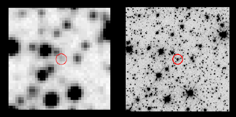
Figure 1: Each image represents a $25\arcsec\times 25\arcsec$ field centered on the lensed source object. The image on the left is from the 300 sec MACHO R-band template observation, and on the right is a 4 x 500 sec combined HST R-band image. The lensed source is in the center of each image, and is indicated by the circle. North is up and east is to the left.

Microlensing Alert MACHO 96-LMC-2 was detected and announced on Oct 3, 1996, with the MACHO object at an observed magnification of $A\sim 1.8$. The source for this event is located at $\alpha=$ 05:34:44.437, $\delta=-$70:25:07.37 (J2000), in the south-east extreme of the LMC bar. This object was constant at $V=19.42\pm 0.15,(V-R)=-0.03\pm 0.10$ in $\sim 700$ observations over the 4.2 years preceding this brightening, where these magnitude errors are dominated by uncertainty in the calibration of the MACHO database Alcock et al. (1999b). The MACHO ID number for this star is $11.8871.2108$. A $25\arcsec\times 25\arcsec$ postage stamp, taken from the MACHO R-band template observation of this field and centered around the lensed object, is presented in Figure 1.

Nightly observations were requested on the CTIO 0.9m telescope as part of the Global Microlensing Alert Network (GMAN) microlensing follow-up program (Alcock et al. (1997b, 1999a, 2000a)). Data were obtained in both $B$ and Kron-Cousins $R$ for the duration of this event. Final sets of baseline observations were made $\sim 800$ days ($\sim 8$ times the duration of the event) after the peak. An additional set of observations was made at the UTSO 0.6m telescope. However, closure of the telescope in 1997 prevented baseline measurements from this site.

After the event, cycle-7 HST images were taken with the target star centered in the Planetary Camera of HST instrument WFPC2. These integrations included four 500 second exposures in each of three bands $V$, $R$, and $I$. The images were combined using the IRAF routine imcombine, along with a sigma clipping algorithm to remove cosmic rays. Aperture photometry was performed on all stars using the DaoPhot package Stetson (1994a), with centroids derived from a PSF fit. We used a 0.25$\arcsec$ aperture, and corrected to a 0.5$\arcsec$ aperture using the brightest stars in the field. We corrected for the charge transfer effect and calibrate the magnitudes using the ?) calibrations. A portion of the combined R-band image of the WFPC2-imaged field around event 96-LMC-2 is presented in Figure 1.

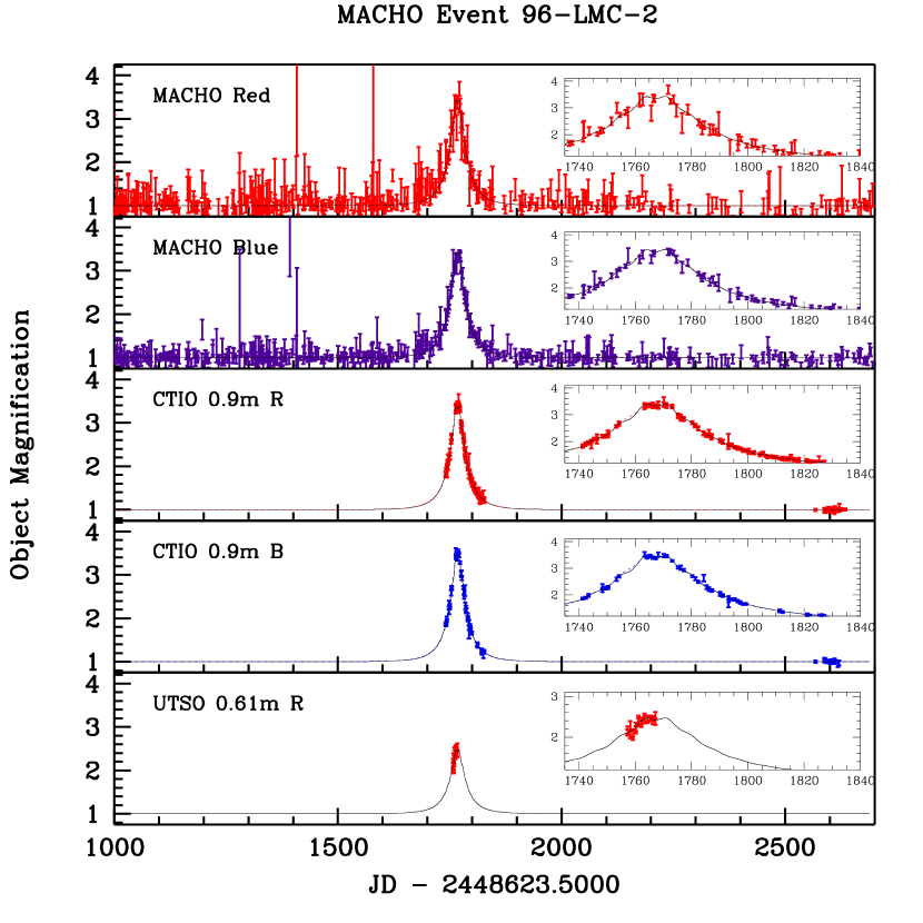
Figure 2: The light curve of event 96-LMC-2. The panels show the observed brightening as a function of time, with passbands and sites as indicated. The solid line represents the best “xallarap” fit X1, and the dotted line fit X2. Insets are provided to better view the region with the strongest binary source signal. The UTSO data are only plotted with the X1 fit curve.

The MACHO/GMAN data for 96-LMC-2 are presented in Figure 2. The MACHO data were reduced with MACHO’s standard photometry package SoDOPHOT, with minimum errors of 0.014 added in quadrature. The CTIO and UTSO data were simultaneously reduced with the ALLFRAME package Stetson (1994b), and the error estimates are multiplied by a factor of 1.5 to account for global systematics (such as flat-fielding errors and the swapping of CCD detectors) in the time series of data.

3 Microlensing Fits

3.1 Standard Microlensing

Standard microlensing fit parameters, including the effects of unlensed contributions to the source baseline flux, are presented in Table 1. These include

• $t_{\rm 0}$, the time of closest approach of lens to source-observer line of sight,

• $\widehat{t}$, the Einstein ring diameter crossing time,

• $u_{\rm min}$, the lens impact parameter in units of the Einstein ring radius.

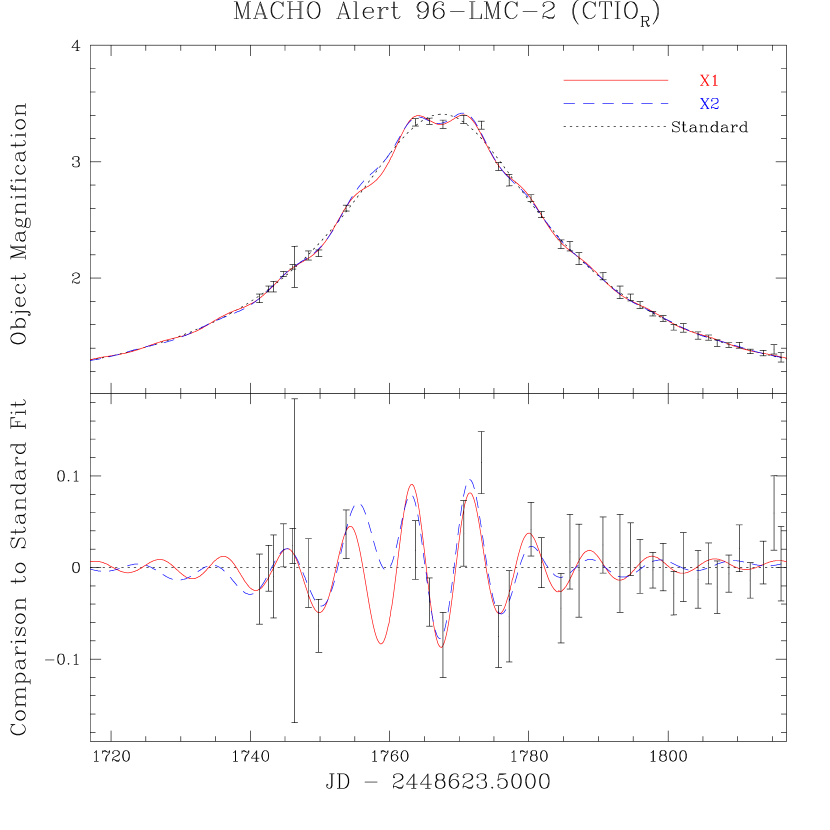
Figure 3: The CTIO R-passband light curve of 96-LMC-2. The top panel displays the 3 fits performed on the complete time-series of data, along with the CTIO R-band data in 1-day bins. The dotted line represents the best standard fit, and the solid and dashed lines the most significant and second most significant xallarap fits X1 and X2, respectively. The bottom panel indicates the residuals of each fit and the data around the standard microlensing fit.

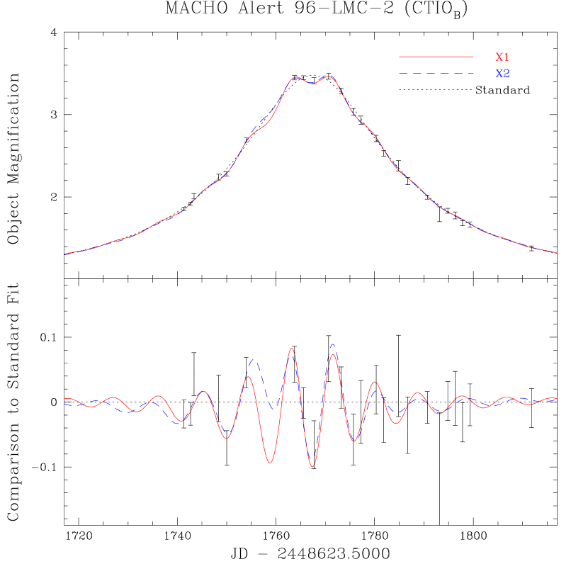
Figure 4: Same as Figure 3, except with the CTIO B-band light curve.

We also include 5 additional blending parameters, one $f$ for each passband of observations. In each case, $f$ represents the fraction of the object’s baseline flux which was lensed. The $\chi^{2}/d.o.f$ for this fit is 0.91, formally an acceptable fit. However, there are periodic residuals around this smooth fit, especially in the CTIO data. We have plotted these residuals for the CTIO R and B passbands in Figure 3 and Figure 4, respectively.

3.2 Binary Source (Xallarap) Microlensing

Fitting this event to an orbiting binary source does provide significant improvement over the standard blended fit. We follow the formalism of ?) for the binary source solution. In particular, we use the fit parameters:

• $\tilde{t}_{b}$, the time of closest approach of the lens to the source system center of mass,

• $t_{\rm E}$, the lens’ Einstein radius crossing time,

• $\tilde{b}$, the lens’ impact parameter with respect to the source system center of mass, in units of the lens’ Einstein radius projected into the source plane,

• $\tilde{\alpha}$, the angle between the lens trajectory and the $x$ source axis,

• $\tilde{f}_{1}$, the total binary flux fraction of source 1,

• $\tilde{m}_{1}$, the total binary mass fraction of source 1,

• $\tilde{\rho}$, the orbital semi-major axis in units of the lens’ projected Einstein radius,

• $\tilde{\beta}$, the orbital inclination,

• $\tilde{T}$, the orbital period in days,

• $\tilde{\xi}_{0}$, the orbital phase at time $\tilde{t}_{b}$,

and one $f$ for each passband of observations, an additional 8 parameters compared to the standard blended microlensing fit. Finally, we assume zero eccentricity circular orbits for the sources, meaning inclination angle $\tilde{\gamma}$ from ?) is redundant, and is set to zero in these fits.

We find 2 minima in this parameter space, separated by $\Delta\chi^{2}\sim 1$. Our most significant model is labeled X1, and our second most significant is X2. These fits are a further $\Delta\chi^{2}=72$ from the standard microlensing fit, which we are extremely unlikely to arrive at by chance, even given our additional 7 constraints. Xallarap fit parameters are presented in Table 2. Fit X1 indicates a primary which contributes $\sim 100\%$ of the light, a dark secondary, and an orbital period of $T=9.22\pm 0.21$ days. The second fit X2 yields a binary source of similar mass and brightness stars, and $T=21.2\pm 0.54$ days. These fits and the residuals of these fits around the standard microlensing fit are plotted along with the data for the CTIO R and B passbands in Figure 3 and Figure 4, respectively.

We have investigated whether or not the sources contribute significantly different flux fractions in the red and blue, by allowing different $\tilde{f}_{1}$ fractions for the red and blue passbands. Providing this additional constraint leads to a $\Delta\chi^{2}=-0.24(-0.50)$ for fit X1 (X2), indicating this improvement is formally significant at only the $37\%(52\%)$ confidence level. For the fit X1 class, the secondary source is dark in both red and blue, to within the reported accuracy of our photometry. For the X2 class, the best fit $\tilde{f}_{1r}/\tilde{f}_{1b}$ is 1.02. In the following we assume $\tilde{f}_{1r}=\tilde{f}_{1b}=\tilde{f}_{1}$.

The binary source fits for this event are plotted with the data in Figure 2. Due to the different blend fractions for these fits, the observed object magnification (as opposed to the lensed source magnification) is plotted as a function of time. It is apparent that without the GMAN follow-up photometry, there would be little support for the binary source interpretation. In fact, $80\%$ of the $\Delta\chi^{2}$ between the standard fit and fit X1 is contributed by the GMAN data.

3.2.1 Colors of the Lensed Objects

The source object’s brightness is well constrained with our $V,R,$ and $I$ HST images. We use the image subtraction method of ?) to locate the lensed source in the MACHO images to within 0.1” (2 PC pixels). Image registration allows us to uniquely determine the centroid of the lensed source in the HST image. This lensed flux aligns with an object with $V=19.46\pm 0.02,(V-R)=0.00\pm 0.03,(V-I)=0.12\pm 0.03$, where the errors represent the quadratic sum of Poisson noise and an adopted error of $2\%$ for our HST magnitudes. Within $1^{\prime\prime}$ of this source there are at least 2 neighbors, which contribute about $20\%$ of the flux within this region.

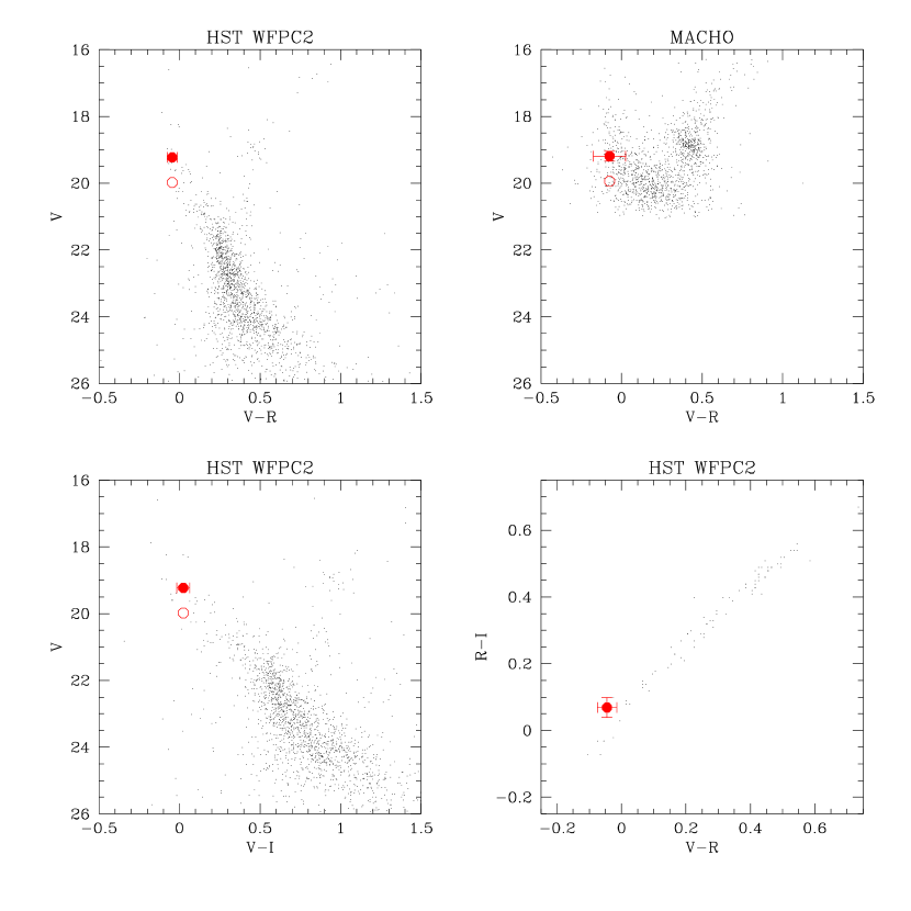
Figure 5: Color-magnitude and color-color diagrams of the field surrounding event 96-LMC-2. The lensed object is indicated with a filled circle. The HST CMDs are constructed from cycle-7 observations with the target star centered on the Planetary Camera chip of the WFPC2. The MACHO CMD is taken from a subsection of the template observation of this field. Error bars indicate the uncertainties in each respective CMD. This object resides near the upper main sequence of the LMC field. We indicate with an open circle the region of the CMD where 2 equal brightness stars must be drawn from to create the observed object.

Color-magnitude diagrams (CMDs) incorporating $\sim$1800 objects from the Planetary Camera chip of the WFPC2, and a region surrounding the lensed object in the MACHO focal plane, are displayed in Figure 5. The lensed object identified in each respective CMD is indicated with the filled circle. We have corrected the CMDs for reddening, using a characteristic LMC reddening in the bar of $E(B-V)=0.07\pm 0.01$ (e.g., Olsen (1999) and Holtzman et al. (1999)) and the Landolt extinction coefficients of ?). The intrinsic magnitude and colors of the source star are $V=19.23\pm 0.04,(V-R)=-0.04\pm 0.03,(V-I)=0.02\pm 0.03$.

The CMDs in Figure 5 indicate the source lies very close to the main sequence in this region of the LMC. There appears to be a slight excess of flux in the $I$ passband, as can be seen in the $(V-R),(R-I)$ and $(V-I),V$ diagrams. There is no apparent excess in the $(V-R),V$ diagram, suggesting this is an infrared excess. Given the direction of the reddening vector in the $V,R$, and $I$ passbands, this marginal excess cannot be a feature of reddening. This could possibly be due to the lens itself, or in the context of model X1, a signature of the dark companion to the primary. We also indicate in Figure 5 the region 0.75 mag below the lensed object with an open circle, which would be the location of a single component of this object if it were a blend of equal brightness stars, as model X2 suggests.

3.2.2 Properties of the Binary System

We next attempt to estimate the mass of an object with the colors determined above. Since this object appears on the upper main sequence, it is likely to have higher metallicity than the majority of the field stars in this location. Here we consider ?) isochrones for $z=0.008$. For model class X1, the best fits to the colors and apparent magnitude of the star come from objects with $\log({\rm age[yr]})=8.7-8.8$, $M=2.1\pm 0.1{\rm M}_{\odot}$. In the case of model X2, we require a single object $0.75$ mag dimmer than our observed object. Using the same isochrones, we find a wider range in acceptable star age, $\log({\rm age[yr]})=8.5-8.8$, and a range in mass of $M=1.9\pm 0.1{\rm M}_{\odot}$.

The original fits to model X1 yielded $\tilde{m}_{1}\sim\tilde{f}_{1}\sim 0$. In the case of $\tilde{f}_{1}=0$, we are not able to fit model parameters $\tilde{m}_{1}$ and $\tilde{\rho}$ individually, but can only constrain their product $\tilde{m}_{1}~{}*~{}\tilde{\rho}$. Therefore the fitting process was re–run, setting $\tilde{m}_{1}\equiv 0.1$ ($\tilde{m}_{1}=0$ or $\tilde{m}_{1}=1$ imply non–existent secondaries) and fitting for $\tilde{\rho}$. Therefore fit X1 has 1 more degree of freedom than X2. The product $\tilde{m}_{1}~{}*~{}\tilde{\rho}$ was similar to that found in the original model. To explore the range of companions to the $2.1{\rm M}_{\odot}$ primary, we consider a “light” dwarf secondary of $0.1{\rm M}_{\odot}$, henceforth fit X1a, and a “heavy” white dwarf or neutron star secondary of $1.4{\rm M}_{\odot}$, fit X1b. Making these assumptions fixes $\tilde{m}_{1}$ and allows us to extract an associated $\tilde{\rho}$. The resulting parameters $\tilde{m}_{1}$ and $\tilde{\rho}$ for fits X1a and X1b are also listed in Table 2.

Knowing the total mass of the system and orbital period allows us to solve for the physical Keplerian parameters of the binary source. We find semi-major axes of 0.11, 0.13, and 0.23 AU, and circular velocities of 132, 154, and 120 $\,{\rm km\,s^{-1}}$, for fits X1a, X1b, and X2, respectively.

3.2.3 Constraints on the Lensing Object

Xallarap fit parameter $\tilde{\rho}$ relates the scale of the lens’s projected Einstein radius ($\widehat{R}_{\rm E}$) to the binary’s semi-major axis. The derivation above allows us to express this value in AU, and the results are presented in Table 3. This effectively leads to a measurement of the lens proper motion

$$\mu={v_{\rm\perp}\over D_{l}}={\widehat{R}_{\rm E}\over t_{\rm E}D_{s}}.$$ (1)

To find the velocity of the lens projected to the LMC ($\widehat{v}$), we assume a LMC distance modulus of 18.5, or a distance of 50 kpc. We further assume the source is 1 scale height behind the midplane of the LMC disk (see below). The values of $\mu$ and $\widehat{v}$ for each of our fits are presented in Table 3. The error bars on these values do not incorporate uncertainty in the distance to the LMC.

The proper motion measurement allows a one-parameter family of solutions relating the lens mass and distance

$$M_{l}={\mu^{2}t_{\rm E}^{2}c^{2}\over 4G}{D_{s}x\over 1-x}\ ,$$ (2)

where $x$ is the ratio of lens to source distances, $D_{l}/D_{s}$.

With some knowledge of the kinematics of sources and lenses, we can estimate a most likely distance for the lensing object, given our measured $\widehat{v}$. This directly leads to an estimate of the lens mass from Equation (2). This is performed in a manner similar to ?) and ?) for each of the results from models X1a, X1b, and X2. We use the following representation of the Galactic-LMC system: the Galactic halo is represented by Model S of ?); we use the preferred LMC disk model of ?), with a scale-height of 300 pc, tilt of 30 $\deg$ from face-on, central surface density of 190 ${\rm M}_{\odot}$/pc², and we assume the source to be 1 scale height behind the midplane; the Solar velocity in Galactic X, Y, Z is (9, 231, 16) $\,{\rm km\,s^{-1}}$; the LMC velocity is (53, -160, 162) $\,{\rm km\,s^{-1}}$, with isotropic random velocities of 22 $\,{\rm km\,s^{-1}}$ (e.g., Graff et al. (2000)) in each direction. For the LMC halo, we assume a similar profile to the Galactic halo, with a central density of $0.0223{\rm M}_{\odot}{\rm pc}^{-3}$, core radius of $2\,{\rm kpc}$, and velocity dispersion of $50\,{\rm km\,s^{-1}}$. We truncate this halo at $11\,{\rm kpc}$. We note the details of the Galactic and LMC models do not qualitatively alter our conclusions.

We find in each analysis that a lens residing in the LMC is preferred to a Galactic halo lens, although only marginally so in fit X1b. In particular, for fit X1a the likelihood of measuring our value of $\widehat{v}_{X1a}=18.3\,{\rm km\,s^{-1}}$ is dominated by the LMC disk model. For this fit, a LMC disk lens is 7 times more likely than a LMC halo lens, and $>950$ times more likely than a Galactic halo lens. We also point out that secondaries less massive than $0.1{\rm M}_{\odot}$ become increasingly unlikely, as decreasing the mass of the secondary leads to a lower lens $\widehat{v}$. In this model, $\widehat{v}_{X1a}$ already is drawn from the low velocity tail of the LMC disk probability distribution. As an example, a secondary of approximately Jupiter mass would imply a lens velocity projected to the LMC of $\sim 0.2\,{\rm km\,s^{-1}}$, clearly in contradiction to the LMC disk likelihood profile in Figure 6. For fit X1b, we find $\widehat{v}_{X1b}=188\,{\rm km\,s^{-1}}$, which is most likely to come from our model of the LMC halo, although it is only 4 times as likely as a Galactic halo lens. In this case, a LMC disk lens is ruled out at high confidence. We note that such a LMC halo population has yet to be detected directly. Given the broad range in secondary mass, and hence the binary’s semi-major axis, explored between fits X1a and X1b, we conclude this model favors a lens associated with the LMC. With our model X2, we find $\widehat{v}_{X2}=39.6\pm 6.1\,{\rm km\,s^{-1}}$, whose likelihood is strongly dominated by the LMC disk. Figure 6 shows the probability distributions of $\widehat{v}$ for each component of our Galactic-LMC model. Our measured $\widehat{v}$ for each fit is also displayed with $1-\sigma$ errors. Only in model X1b does a Galactic halo lens appear reasonable.

Our likelihood analysis also yields a probable distance to the lens, and from Equation (2), a mass. These parameters are listed in Table 3 for each model. Model X1a allows the lightest lens mass, $0.057{+0.060\atop-0.036}{\rm M}_{\odot}$ , while models X1b and X2 imply heavier lenses, $0.24{+0.38\atop-0.18}$ and $0.28{+0.33\atop-0.20}{\rm M}_{\odot}$, respectively. We have referenced the low mass isochrones of ?) to determine the expected brightness of a main sequence M-dwarf lens. We use the isochrones for $z=0.004$, and an assumed lens age of 4 Gyr. We find for objects of $M=0.3{\rm M}_{\odot}$, and also for the upper $1-\sigma$ confidence limit $M=0.6{\rm M}_{\odot}$, absolute V magnitudes of 9.9 and 7.6, respectively. At the distances implied by the likelihood analysis, even the most luminous configuration provides negligible flux from the lens compared to the apparent brightness of the source object. A $0.6{\rm M}_{\odot}$ lens at $45\,{\rm kpc}$ leads to an apparent lens magnitude of $V=25.9$, or $0.2\%$ of the source brightness. The apparent I–band brightness of this lens is $I=24.7$, or less than $0.1\%$ of the source brightness in this band. The secondary source is therefore a more likely origin for the possible I–band excess seen in Figure 5. The small lens proper motion of $\lesssim 1$ milli-arcsecond year^-1 implies it will take the next generation of space telescopes to be able to resolve and image the lensing object.

We note that the lens’ location (and therefore its mass) can be more accurately determined with direct spectral observations of the source. In particular, the superposition of primary and secondary spectra can provide a discriminant between models X1 and X2, and lead to a better mass estimate for each object. Similarly, the orbital period can be precisely determined with radial velocity measurements. These observations will constrain the Keplerian parameters more directly than our (necessarily) more complicated microlensing analysis has allowed.

3.3 Alternate Models

In order to gauge the robustness of these conclusions, we have considered several alternate models, including placing the sources at larger distances behind the LMC, and increasing the amount of reddening to the sources.

?) predicts a strong excess in lensed source reddening for models where the LMC is strongly self–lensing. In these models, the source stars must preferentially lie at the back side of the LMC, and thus will have high interstellar reddenings. On the other hand, if the lenses are Galactic dark matter, the reddenings of the source stars will be statistically the same as surrounding stars along the same lines of sight. ?) use HST colors of 8 microlensed source stars to rule out, at the 85% confidence level, a model where all sources are located $\sim$7 kpc behind the LMC disk. However, it is possible that roughly half of the sources may be in the background. Therefore, we consider a model where the lensed sources are $7-9\,{\rm kpc}$ behind the LMC. This leads to an increase in source mass of $\sim 0.1{\rm M}_{\odot}$, and results in projected velocities of $\widehat{v}_{X1a}=18\,{\rm km\,s^{-1}},\widehat{v}_{X1b}=184\,{\rm km\,s^{-1}}$, and $\widehat{v}_{X2}=40\,{\rm km\,s^{-1}}$. The $\widehat{v}$ likelihood profiles for this source location differ significantly from those seen in Figure 6. Most notably, the LMC disk and LMC halo profiles allow a similar range in $\widehat{v}$, with the LMC halo generally preferred over the LMC disk, and median $\widehat{v}\sim 100\,{\rm km\,s^{-1}}$. For the lowest projected velocity (model X1a), the lens is consistent with neither the LMC nor the Galactic likelihood profiles. The LMC halo is the most likely location of the lens in all models, followed by the LMC disk in model X2, and by the Galactic halo in model X1b.

It is also possible the reddening to the sources is larger than our adopted value of $E(B-V)=0.07$. For example, the foreground reddening maps of ?) indicate $E(B-V)=0.12$, while ?) finds typical LMC source star reddenings of $E(B-V)\sim 0.10$. If we assume a higher reddening to the source object of $E(B-V)=0.12$, its intrinsic brightness and colors are $V=19.06,(V-R)=-0.08,(V-I)=-0.05$. For model X1, the primary source would weigh $\sim 2.3{\rm M}_{\odot}$, and for model X2 both sources would weigh $\sim 2.1{\rm M}_{\odot}$. Here we find $\widehat{v}_{X1a}=17\,{\rm km\,s^{-1}},\widehat{v}_{X1b}=181\,{\rm km\,s^{-1}}$, and $\widehat{v}_{X2}=41\,{\rm km\,s^{-1}}$, whose relative likelihoods can be evaluated using Figure 6. This change has more important implications for the source mass than for the projected velocities, and the likelihood results are similar to those from the standard analysis.

4 Conclusions

We have measured and characterized a periodic modulation in the lightcurve of microlensing event MACHO 96-LMC-2. We model this event using a single object microlensing a rotating binary source, which provides considerable improvement over a single source model. Possible alternate explanations to this modulation include a single source lensed by a rapidly rotating binary lens, or some variant of stellar pulsation. We do not consider such models. MACHO 96-LMC-2 is not the only time that binary source effects have been detected in a microlensing event. EROS-II event GSA2 Derue et al. (1999) exhibits a similar modulation around the standard microlensing fit. ?) also find a binary source model degeneracy similar to that between our models X1 (dominant source) and X2 (equal brightness sources).

We are able to constrain the projected Einstein radius of the lens ($\widehat{R}_{\rm E}$) in the most significant of our fits to be between 0.54 and 5.5 AU, and its velocity projected to the LMC $\widehat{v}$ to be between 18.3 and 188 $\,{\rm km\,s^{-1}}$. The weakness of this constraint (an order of magnitude!) is due to our lack of knowledge of the mass of the secondary component of the lensed binary system. In this model we have no means to constrain the secondary’s orbit due to its negligible contribution to the system’s brightness. We chose example secondaries separated by an order of magnitude in mass ($0.1{\rm M}_{\odot}$ to $1.4{\rm M}_{\odot}$), leading to order of magnitude constraints on $\widehat{R}_{\rm E}$ and $\widehat{v}$. However, in both cases, a LMC lens is preferred to a Galactic halo lens. For the larger velocity lens (model X1b) the object should come from an as yet undetected LMC halo population, and a Galactic halo lens is not strongly ruled out. The lack of direct evidence for an LMC halo population indicates model X1b is best able to constrain the location of the lens to be out of the LMC disk. Our second most significant model leads to $\widehat{R}_{\rm E}=1.24\pm 0.18$ AU, and $\widehat{v}=39.6\pm 6.1\,{\rm km\,s^{-1}}$. This model also prefers a lens in the LMC, with the likelihood heavily weighted towards the LMC disk. All 3 of these models suggest a sub-solar mass lens, consistent with an M-dwarf star. Our derived values of $\widehat{R}_{\rm E}$, $\widehat{v}$, $M_{l}$, and $D_{l}$ are in good agreement with the characteristic properties of LMC lenses presented in Table 1 of ?).

Alternate models for the source system, including one where the sources lie $7-9\,{\rm kpc}$ behind the LMC, and one where they are reddened by an additional $\Delta E(B-V)=0.05$, were also considered. By placing the sources far behind the LMC, we are unable to discriminate between the LMC disk and LMC halo population of lenses, and can only state that the lens is most likely associated with the LMC system. Additionally, the qualitative conclusions about the location of the lens are found not to be overly sensitive to the amount of reddening to the sources.

The identification of MACHO 96-LMC-2 with a LMC lens population is consistent with the expected LMC self-lensing signal. This single event microlensing optical depth is $\tau_{A}=1.1\times 10^{-8},\tau_{B}=8.5\times 10^{-9}$ for criteria “A” and “B” in ?), respectively. This is to be contrasted with an expected self-lensing optical depth of $\tau=1.6\times 10^{-8}$ for the LMC disk and $\tau=1.7\times 10^{-8}$ for the MACHO component of our model LMC halo Alcock et al. (2000b). It is also possible that MACHO LMC-9 is due to LMC self-lensing Alcock et al. (2000a), although we caution this interpretation is based on a caustic crossing resolved with only 2 observations, and other interpretations are possible. LMC-9 is excluded from event set A in ?), and has an optical depth of $\tau_{B}=9.3\times 10^{-9}$. The expected LMC self-lensing signal due to these 2 events is thus likely to lie within the range $1.1\times 10^{-8}<\tau<1.8\times 10^{-8}$. This is approximately half of the expected LMC self-lensing rate. Thus the combined optical depths alone do not implicate the LMC as the host for the majority of the microlenses, as originally suggested by ?).

?) take the ensemble of events LMC-9 and 98-SMC-1 and argue that the existence of even a few LMC self-lensing events suggests an LMC halo interpretation of all LMC microlensing. In this context, the appearance of another apparent LMC self-lensing event strengthens the case for significant LMC self-lensing. However, because of the importance of our result for the interpretation of LMC microlensing, we emphasize the bias a study such as this has against revealing a lens residing in our Galactic halo. In particular, a lensed LMC binary source is preferentially more likely to show xallarap modulations if the lens is also in the LMC. To identify Galactic halo lenses, a spectroscopic study of all Magellanic Cloud microlensed sources should be undertaken to assess whether or not the lensed object is, in fact, a binary system. In the case of a positive detection, we may set limits on xallarap modulation in the microlensing lightcurve, and from this a lower limit on the proper motion of the lensing object. As can be seen from Figure 6, Galactic halo lenses start to dominate the likelihood near $\widehat{v}=230\,{\rm km\,s^{-1}}$. A lower limit on $\widehat{v}$ near this value would be highly suggestive of a true halo lens, and thus detection of at least one component of the Galactic dark matter. We suggest such a study of the high magnification event MACHO 99-LMC-2 Becker (1999), whose lightcurve is well covered by the MACHO/GMAN, MOA, MPS, and OGLE microlensing teams.

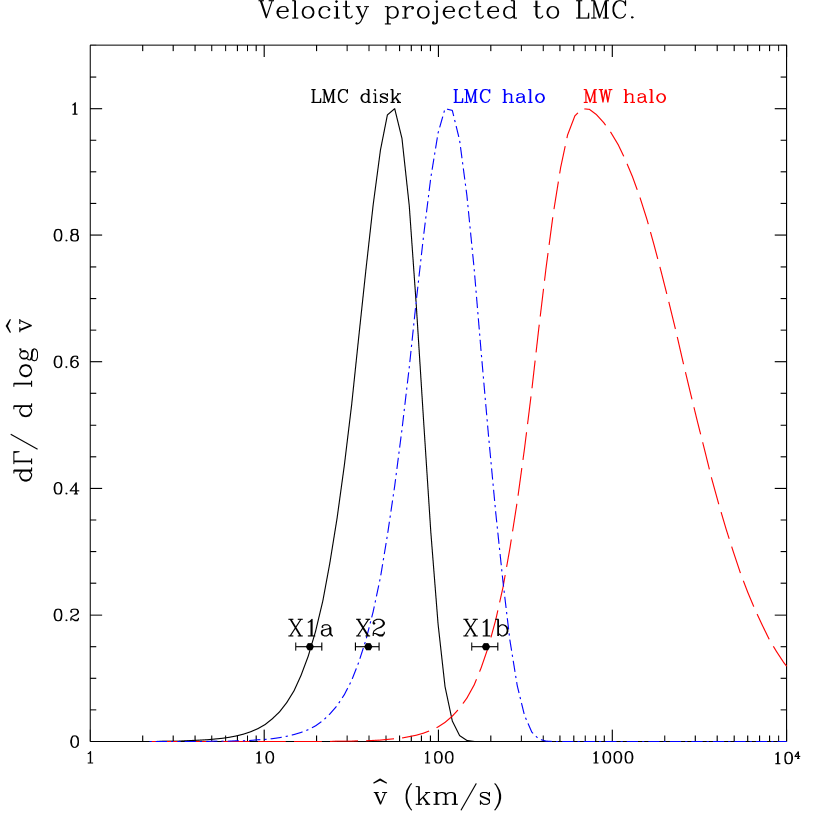
Figure 6: Probability distributions of $\widehat{v}$ for each component of our Galactic-LMC model, described in Sec. 3.2.3. The measured $\widehat{v}$ for models X1a, X1b, and X2 is also indicated, with respective $1-\sigma$ errors. Note in each case, a LMC lens is preferred over a Galactic halo lens, although this preference is weakest for model X1b.

Table 1: Standard Microlensing Fit Parameters

Fit Parameter
$\chi^{2}$ / d.o.f.	1872.31 / 2060
$t_{\rm 0}$	1767.51 (7)
$\widehat{t}$	98.7 (40)
$u_{\rm min}$	0.301 (17)
$f_{MACHO_{R}}$	1.00 (13)
$f_{MACHO_{B}}$	1.00 (13)
$f_{CTIO_{R}}$	0.99 (12)
$f_{CTIO_{B}}$	1.02 (13)
$f_{UTSO_{R}}$	0.76 (33)

Table 2: Xallarap Microlensing Fit Parameters

	X1	X1a	X1b	X2
$\chi^{2}$ / d.o.f.	1799.9 / 2054	$\cdots$	$\cdots$	1800.9 / 2053
$\tilde{t}_{b}$	1767.600 (79)	$\cdots$	$\cdots$	1767.80 (14)
$2*t_{\rm E}$	101.8 (42)	$\cdots$	$\cdots$	108.8 (53)
$\tilde{b}$	0.287 (16)	$\cdots$	$\cdots$	0.246 (19)
$\tilde{\alpha}$	-2.15 (37)	$\cdots$	$\cdots$	0.236 (77)
$\tilde{f}_{1}$	0.000 (29)	$\cdots$	$\cdots$	0.52 (19)
$\tilde{m}_{1}$	0.1	0.045	0.40	0.53 (19)
$\tilde{\rho}$	0.095 (15)	0.208 (33)	0.0237 (39)	0.188 (26)
$\tilde{\beta}$	1.00 (30)	$\cdots$	$\cdots$	1.43 (14)
$\tilde{T}$	9.22 (21)	$\cdots$	$\cdots$	21.22 (53)
$\tilde{\xi}_{0}$	-0.23 (37)	$\cdots$	$\cdots$	0.40 (12)
$f_{MACHO_{R}}$	0.94 (9)	$\cdots$	$\cdots$	0.80 (8)
$f_{MACHO_{B}}$	0.95 (9)	$\cdots$	$\cdots$	0.80 (8)
$f_{CTIO_{R}}$	0.93 (9)	$\cdots$	$\cdots$	0.79 (8)
$f_{CTIO_{B}}$	0.96 (9)	$\cdots$	$\cdots$	0.81 (8)
$f_{UTSO_{R}}$	0.58 (18)	$\cdots$	$\cdots$	0.86 (46)

Table 3: Properties of the Lensing Object

	X1a	X1b	X2
$\widehat{R}_{\rm E}$  (AU)	0.535 (88)	5.50 (91)	1.24 (18)
$\mu~{}~{}(\,{\rm km\,s^{-1}\,kpc^{-1}})$	0.364 (62)	3.73 (64)	0.79 (12)
$\widehat{v}~{}~{}(\,{\rm km\,s^{-1}})$	18.3 (31)	188 (32)	39.6 (61)
$M_{l}~{}~{}({\rm M}_{\odot})$	$5.7{+6.0\atop-3.6}\times 10^{-2}$	$2.4{+3.8\atop-1.8}\times 10^{-1}$	$2.8{+3.3\atop-2.0}\times 10^{-1}$
$D_{l}~{}~{}(\,{\rm kpc})$	$49.6{+0.3\atop-1.0}$	$38.5{+6.5\atop-15.7}$	$49.6{+0.4\atop-1.6}$

References

- Afonso et al. (1999) Afonso, C., et al. 1999, A&A, 344, L63
- Afonso et al. (2000) Afonso, C., et al. 2000, ApJ, 532, 340
- Alcock et al. (1995) Alcock, C., et al. 1995, ApJ, 454, L125
- Alcock et al. (1997a) Alcock, C., et al. 1997a, ApJ, 486, 697
- Alcock et al. (1997b) Alcock, C., et al. 1997b, ApJ, 491, 436
- Alcock et al. (1999a) Alcock, C., et al. 1999a, ApJ, 518, 44
- Alcock et al. (1999b) Alcock, C., et al. 1999b, PASP, 111, 1539
- Alcock et al. (2000a) Alcock, C., et al. 2000a, ApJ, 541, 270
- Alcock et al. (2000b) Alcock, C., et al. 2000b, ApJ, 542, 000
- Alcock et al. (2000c) Alcock, C., et al. 2000c, ApJ, Submitted
- Becker (1999) Becker, A. 1999, IAU Circ., 7188, 1
- Cardelli et al. (1989) Cardelli, J. A., Clayton, G. C., & Mathis, J. S. 1989, ApJ, 345, 245
- Derue et al. (1999) Derue, F., et al. 1999, A&A, 351, 87
- Dominik (1998) Dominik, M. 1998, A&A, 329, 361
- Girardi et al. (2000) Girardi, L., Bressan, A., Bertelli, G., & Chiosi, C. 2000, A&AS, 141, 371
- Gould (1992) Gould, A. 1992, ApJ, 392, 442
- Graff et al. (2000) Graff, D. S., Gould, A. P., Suntzeff, N., Schommer, R. A., & Hardy, E. 2000, ApJ, 540, 211
- Griest & Hu (1992) Griest, K., & Hu, W. 1992, ApJ, 397, 362
- Gyuk et al. (2000) Gyuk, G., Dalal, N., & Griest, K. 2000, ApJ, 535, 90
- Han & Gould (1997) Han, C., & Gould, A. 1997, ApJ, 480, 196
- Holtzman et al. (1995) Holtzman, J. A., Burrows, C. J., Casertano, S., Hester, J. J., Trauger, J. T., Watson, A. M., & Worthey, G. 1995, PASP, 107, 1065
- Holtzman et al. (1999) Holtzman, J. A., et al. 1999, AJ, 118, 2262
- Kerins & Evans (1999) Kerins, E. J., & Evans, N. W. 1999, ApJ, 517, 734
- Olsen (1999) Olsen, K. A. G. 1999, AJ, 117, 2244
- Sahu (1994) Sahu, K. C. 1994, Nature, 370, 275
- Schlegel et al. (1998) Schlegel, D. J., Finkbeiner, D. P., & Davis, M. 1998, ApJ, 500, 525
- Schwering & Israel (1991) Schwering, P. B. W., & Israel, F. P. 1991, A&A, 246, 231
- Stetson (1994a) Stetson, P. B. 1994a, User’s Manual for DAOPHOT II, Dominion Astrophysical Observatory
- Stetson (1994b) Stetson, P. B. 1994b, PASP, 106, 250
- Tomaney & Crotts (1996) Tomaney, A. B., & Crotts, A. P. S. 1996, AJ, 112, 2872
- Zaritsky (1999) Zaritsky, D. 1999, AJ, 118, 2824
- Zhao (2000) Zhao, H. S. 2000, ApJ, 530, 299