[

Position-Space Description of the Cosmic Microwave Background
and Its Temperature Correlation Function

Abstract

We suggest that the cosmic microwave background (CMB) temperature correlation function $C(\theta)$ as a function of angle provides a direct connection between experimental data and the fundamental cosmological quantities. The evolution of inhomogeneities in the prerecombination universe is studied using their Green’s functions in position space. We find that a primordial adiabatic point perturbation propagates as a sharp-edged spherical acoustic wave. Density singularities at its wavefronts create a feature in the CMB correlation function distinguished by a dip at $\theta\approx 1.2^{\circ}$. Characteristics of the feature are sensitive to the values of cosmological parameters, in particular to the total and the baryon densities.

]

The cosmic microwave background (CMB) radiation provides the best probe today of the early universe and a number of fundamental astrophysical constants [1, 2, 3, 4, 5, 6, 7]. Dynamical evolution of primordial perturbations manifests itself in the form of “acoustic peaks” in the CMB temperature angular power spectrum $C_{l}$. After over a decade of studies, the physical content of the peaks has become qualitatively understood [8, 9, 10, 11]. Nevertheless, one has to rely on standard numerical codes [12, 13] to establish a quantitative connection between the CMB anisotropy pattern and cosmological parameters. This connection is particularly important now that high-precision CMB measurements have become reality.

In this letter we show that previously unnoticed interesting phenomena are unraveled by considering the radiation-matter dynamics in position rather than Fourier space. Traditional CMB anisotropy analyses begin with the Fourier expansion of spatial inhomogeneities and studying time evolution of individual Fourier modes [16, 17, 18]. The position space approach, while offering a formally equivalent description, differs in its physical interpretation, associated calculational methods, and its implications for data analysis. As we show here, a new side of CMB physics is revealed in position space. One goal of our work is a deeper physical understanding of both the CMB power spectrum $C_{l}$ and the angular correlation function $C(\theta)$. We demonstrate that acoustic evolution of perturbations before recombination, as viewed in position space, produces sharp features in $C(\theta)$. These signatures not only provide a simple interpretation of the acoustic peaks, but they may also enable fast and accurate extraction of cosmological parameters directly from $C(\theta)$.

As a simplified model for the essential physical processes, we consider the evolution of potential and density perturbations in gravitationally interacting photon-baryon and cold dark matter fluids. We use the conformal Newtonian gauge [18, 19] to describe gravity and assume adiabatic (isentropic) primordial fluctuations as preferred by the present data [14, 15] and the simplest inflationary models. The photons are assumed to be tightly coupled to electrons and baryons by Thomson scattering until recombination at redshift $z_{\rm rec}\sim 1100$. Neutrinos are treated like photons. The disregard of neutrino free-streaming and photon diffusion introduces a $10\%-20\%$ error [20, 21] for CMB temperature anisotropy. This model is helpful for developing understanding. Our numerical results for the correlation function and the angular spectrum are obtained a full calculation with CMBFAST [12] including all relevant effects.

Long before recombination during the radiation era, the growing mode of gravitational potential perturbation is described in Fourier space by $\phi({\bf k},\tau)=3\left[\sin(q)/q^{3}-\cos(q)/q^{2}\right]\phi_{0}({\bf k})$, $q\equiv kc_{s}\tau$, where $\tau$ is conformal time, ${\bf k}$ is the wave vector corresponding to a comoving coordinate ${\bf r}$, and $c_{s}=1/\sqrt{3}$ is the speed of sound in the radiation era [16]. A delta function primordial perturbation $\phi({\bf r},\tau\to 0)=\delta^{(3)}({\bf r})$ is represented in $k$-space by constant initial amplitude $\phi_{0}({\bf k})=1$. Fourier transforming the resulting $\phi({\bf k},\tau)$ we obtain the three-dimensional Green’s function for the gravitational potential in the radiation dominated epoch,

$$\phi^{(3)}(r,\tau)={3\over 4\pi}\,(c_{s}\tau)^{-3}\,\theta(c_{s}\tau-r)\,,$$ (1)

where $\theta(x)\equiv\{1,\,x>0;~{}0\ \mbox{otherwise}\}$. Eq. (1) illustrates the essential property of the position-space Green’s functions—the perturbation is localized within the acoustic sphere, with a sharp edge at the sound horizon $r=S(\tau)\equiv\int_{0}^{\tau}c_{s}(\tau^{\prime})\,d\tau^{\prime}$.

When cold dark matter (CDM) and baryons are taken into account, we split the total gravitational potential $\phi=\phi_{r}+\phi_{c}$ into a part connected to the photon-baryon plasma, $\phi_{r}$, and a part due to the CDM, $\phi_{c}$ . The sources of the potentials $\phi_{r}$ and $\phi_{c}$ are given respectively by the radiation-baryon and CDM energy densities relative to the net zero-momentum hypersurfaces, the analogues of Bardeen’s [16] gauge-invariant density variable $\epsilon_{m}$. The potentials $\phi_{r}$ and $\phi_{c}$ unambiguously determine the values of all the density and velocity perturbations in our model [22]. Their evolution is described by a pair of coupled equations,

$$\ddot{\phi}_{r}+{\textstyle\sum\nolimits_{i=r,c}}(A_{ri}\dot{\phi}_{i}+B_{ri}\phi_{i}) = c_{s}^{2}\,\nabla^{2}\phi_{r}\ ,$$ (2)

$$\ddot{\phi}_{c}+{\textstyle\sum\nolimits_{i=r,c}}(A_{ci}\dot{\phi}_{i}+B_{ci}\phi_{i}) = 0$$ (3)

where $A_{ij}$ and $B_{ij}$ are simple rational functions of $\tau$ [22].

The first of eqs. (2) shows that a primordial isentropic perturbation at a point propagates as a spherical acoustic wave in the photon-baryon plasma with the sound speed $c_{s}^{2}=dp_{\gamma}/d(\rho_{\gamma}+\rho_{\rm b})=(1/3)/[1+(3\rho_{\rm b})/(4\rho_{\gamma})]$, where $\rho_{\gamma}$ and $\rho_{\rm b}$ are the photon and baryon mean energy densities. As the sound wave passes by, its gravitational effect perturbs the CDM causing it to evolve as described by the second of eqs. (2). Since perturbations propagate differently in the radiation and the CDM components, inhomogeneities do not remain isentropic for $\tau>0$ .

We integrate eqs. (2) numerically along their characteristics starting from the radiation-era solution (1) at $\tau_{\rm init}\simeq 10^{-4}\tau_{\rm rec}$, and increasing the space-time grid spacing with time in proportion to the acoustic horizon size $S(\tau)$. It is convenient to solve eqs. (2) in only one spatial dimension with the initial conditions $\phi^{(1)}(x)\to\delta(x)$ and vanishing entropy perturbation as $\tau\to 0$. The resulting one-dimensional, or plane-parallel, Green’s function for the total potential, $\phi^{(1)}(x,\tau)$, is related to the conventional transfer function $\phi(k,\tau)$ as $\phi(k,\tau)=\int\phi^{(1)}(x,\tau)\,e^{-ikx}dx$. The potential Green’s function in three dimensions equals $\phi^{(3)}(r,\tau)=-(2\pi r)^{-1}\partial\phi^{(1)}(r,\tau)/\partial r$. A superscript “$(1)$” will be used for any quantity (e.g. density perturbation or temperature anisotropy) obtained from the isentropic initial condition $\phi(x,\tau\to 0)=\delta(x)$, and such quantities will similarly be referred to as “Green’s functions.” The Fourier transform of any Green’s function gives the corresponding $k$-space transfer function.

Fig. 1 shows the result for an effective temperature Green’s function $\Delta^{(1)}_{\rm eff}(x)$ describing the combined intrinsic and gravitational redshift contributions to CMB temperature anisotropy.

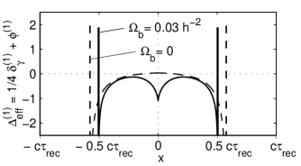
FIG. 1.: The position space transfer function for the intrinsic ($\frac{1}{4}\delta_{\gamma}$) plus gravitational redshift contributions to the CMB temperature anisotropy $\Delta T/T$ at recombination, for $\Omega_{\rm m}=0.35$, $\Omega_{\Lambda}=0.65$, and $h=0.65$. The vertical spikes represent the wave-front delta function singularities described in the text. Baryon drag effects are evident from comparing the solid and dashed lines.

Within our tight coupling assumption, it contains delta function singularities at the wave fronts given by $(3/4)\left[1+(3\rho_{\rm b})/(4\rho_{\gamma})\right]^{-1/4}\delta\left(|x|-S\right)$, where $S(\tau)\equiv\int_{0}^{\tau}c_{s}(\tau^{\prime})d\tau^{\prime}$. The contribution of the delta function to $\int\Delta^{(1)}_{\rm eff}(x,\tau_{\rm rec})\,dx$ exceeds the absolute value of the contribution from the regular part by $\sim 40\%$, showing that the singularities play a major role in CMB anisotropy.

The massive baryons coupled to the radiation fluid reduce the sound speed that decreases the acoustic horizon at recombination. They also drag radiation out of the $x=0$ region in Fig. 1 being repelled by a kink in CDM potential $\phi_{c}^{(1)}$ at $x=0$. This effect causes the prominent “gully” in the middle of the transfer function in Fig. 1.

The peculiar features of the position space transfer functions are manifested in the angular correlation function

$$C(\theta)\equiv\left\langle\Delta T({\bf\hat{n}}_{1})\Delta T({\bf\hat{n}}_{2})\right\rangle=\sum_{l}{(2l+1)\over 4\pi}\,C_{l}P_{l}(\cos\theta)\,,$$ (4)

where $\Delta T({\bf\hat{n}}_{i})$ is the temperature anisotropy in the direction ${\bf\hat{n}}_{i}$, and $\theta$ is the angle between ${\bf\hat{n}}_{1}$ and ${\bf\hat{n}}_{2}$ . The connection between $C(\theta)$ and the Green’s functions may be illustrated in the large angle limit when $\Delta T({\bf\hat{n}}_{i})/T\approx\Delta_{\rm eff}({\bf\hat{n}}_{i},\tau_{\rm rec})\equiv\frac{1}{4}\delta_{\gamma}+\phi$, $\delta_{\gamma}\equiv\delta\rho_{\gamma}/\rho_{\gamma}$, for $\theta$ exceeding a few degrees. Writing each $\Delta T({\bf\hat{n}}_{i})$ as the convolution of the Green’s function in Fig. 1 with a primordial potential field $\phi_{0}$, assuming that recombination occurs instantaneously, and averaging over the primordial fluctuations with power spectrum $\langle\phi_{0}({\bf k}_{1})\phi_{0}({\bf k}_{2})\rangle\propto\delta^{(3)}({\bf k}_{1}+{\bf k}_{2})k^{n_{s}-4}$, we get

$$C(\theta)\propto\int dx_{1}\,\Delta_{\rm eff}^{(1)}(x_{1})\int dx_{2}\,\Delta_{\rm eff}^{(1)}(x_{2})\,K(x_{1}+x_{2},\theta)\,,$$ (5)

where $K$ is an analytically known function of $x_{1}+x_{2}$, angle $\theta$, the comoving distance to CMB photosphere $R$, and the spectral index $n_{s}$ [22]. The exact formula for $C(\theta)$ applicable to subdegree scales should also include Doppler and integrated Sachs-Wolfe effects and integration along the line of sight [12]. Eq. (5) neglects these contributions but is sufficient to give a good qualitative description of the effects considered below.

From eq. (5), the delta function singularities produce a singular $C(\theta)$ behavior in the vicinity of $\theta_{s}\equiv 2\arcsin(S/R)$, where $S\equiv S(\tau_{\rm rec})\simeq 140$ Mpc is the acoustic horizon size at recombination. For a flat universe and the scale-invariant power spectrum $n_{s}=1$, $C(\theta)-C(\theta_{s})\sim-\Delta s\ln\left|\Delta s\right|$, $\Delta s\equiv\sin(\theta/2)-S/R$. When the two observed points come into acoustic contact at the critical angle $\theta_{s}$, $dC(\theta_{s})/d\theta=+\infty$ in the instantaneous recombination approximation. At this angular separation, a spherical sound wave emitted at $\tau=0$ from the point halfway between the observed points on the photosphere has, by recombination, just reached the two observed points separated by a distance $2S$.

Paradoxically, the initial acoustic contact anti-correlates the temperature fluctuations causing a dip in the correlation function just below $\theta_{s}$ . As evident from Fig. 2 , the dip is also present in the full result obtained from a CMBFAST calculation (wide solid line) although smoothed by the Silk damping [23] and the finite thickness of the recombination photosphere. An anomaly in the correlation function at this angular separation was pointed out earlier in [24] and [25]. At even smaller angles the correlation function rises steeply. The dip occurs when the comoving separation of the observed points on the photosphere is about $2S\simeq 280$ Mpc, providing a “standard ruler” in the early universe. The comoving distance to the photosphere $R$ and thus the observed angle $\theta_{s}$ are determined by the rate of the subsequent Hubble expansion and by the cosmic curvature, which both depend on the total density parameter $\Omega$.

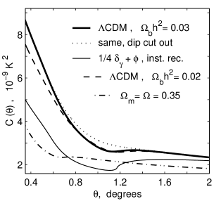
FIG. 2.: Angular CMB temperature correlation function. The parameters of the $\Lambda$CDM model are $\Omega_{\rm m}=0.35$, $\Omega_{\Lambda}=0.65$, $h=0.65$, $n_{s}=1$. For this set of parameters and the displayed $\Omega_{\rm b}h^{2}$ values, $\theta_{s}\simeq 1.17^{\circ}~{}\mbox{and}~{}1.22^{\circ}$. The thin solid curve is calculated using eq. (4). All the other plots are obtained in full CMBFAST calculation, except for the dotted line that artificially cuts the dip for its Fourier analysis in Fig. 4. The whole feature in $C(\theta)$ is shifted to smaller angles in the open model (dash-dotted line). Baryon density variation modifies the slope for $\theta<\theta_{s}/2$ (dashed vs. solid line).

The dash-dotted line in Fig. 2 demonstrates the shift in the visible location of the dip for an open model.

What is the physical origin of the dip in the correlation function at the acoustic contact? According to our earlier discussion, $\Delta_{\rm eff}^{(3)}(r)=-(2\pi r)^{-1}\partial\Delta_{\rm eff}^{(1)}/\partial r$, which contains the derivative of a delta function. When convolved with the primordial potential field $\phi_{0}$, $\delta^{\prime}(r-S)$ relates $\Delta T({\bf r})$ to the gradient of $\phi_{0}({\bf r})$. The vectorial nature of ${\bf\nabla}\phi_{0}$ results in contributions of opposite signs to the temperature of two points located at distance $S$ in opposite directions.

A larger primordial power spectrum $n_{s}$ leads to a greater magnitude of all small-scale features in the correlation function. In the instantaneous recombination approximation, $C(\theta)-C(\theta_{s})$ varies as $\Delta s/(1-n_{s})$ for $n_{s}<1$ and $\Delta s/|\Delta s|^{n_{s}-1}$ for $n_{s}>1$. Thus, the dip at $\theta=\theta_{s}$ is enhanced for $n_{s}>1$ and suppressed for $n_{s}<1$.

For $\theta\lesssim\theta_{s}/2$ the correlation function slope becomes sensitive to the baryon density $\Omega_{\rm b}$. This can be seen from comparing the dashed and the solid lines in Fig. 2. At such a small angular separation, the Doppler and ISW effects provide significant contribution to the temperature correlation. Nevertheless, the $\Omega_{\rm b}$ dependence is largely determined by the same intrinsic plus gravitational redshift contributions shown in Fig. 1. It is the interference of the baryon induced “gully” in the middle of one of the transfer functions in eq. (5) and the delta function contributions of the other that causes the steeper $C(\theta)$ rise at $\theta\lesssim\theta_{s}/2$. The effect is almost linearly proportional to $\Omega_{\rm b}h^{2}$ and may be useful for measuring the baryon density value using CMB data.

The finite extent of the position-space Green’s functions results in oscillations in their Fourier transforms, the $k$-space transfer functions. These oscillations appear as the famous acoustic peaks in the CMB angular spectrum $C_{l}$ . The characteristic period of the oscillations is $\Delta l=\pi R/S\simeq 300$ for $\Omega_{\rm m}=0.35$, $\Omega_{\Lambda}=0.65$, and $h=0.65$. The wavefront and $x=0$ Green’s function singularities in Fig. 1 do not map directly to a particular distinct feature in $C_{l}$ spectrum because they are completely delocalized by Fourier transformation.

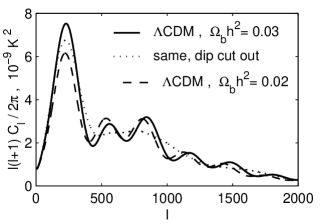
FIG. 3.: Angular power spectra for the $\Lambda$CDM models of Fig. 2. The dotted line gives $C_{l}$ corresponding to the correlation function of the first model with the dip cut out.

An interesting connection between features in $C(\theta)$ and the acoustic peaks in $C_{l}$ is established by artificially cutting out the dip in $C(\theta)$ and replacing it by a smooth interpolation with no local minimum as shown by the dotted line in Fig. 2. Fig. 3. shows that this operation eliminates all the acoustic peaks besides the first one. The first peak is closely connected with the sharp rise in $C(\theta)$ at $\theta<\theta_{s}$. Increasing the baryon density we increase the magnitude of the slope of $C(\theta)$. The magnitude of the first peak grows accordingly (dashed vs. solid lines in Fig. 3) leading to the known [10] reduction in the ratio of second to first acoustic peaks.

In conclusion, the Green’s function method provides a promising alternative to the conventional Fourier analysis of perturbations in the early universe. It offers new analytical methods and intuition for the familiar phenomena such as the acoustic oscillations and the dependence of peak ratios on $\Omega_{\rm b}h^{2}$. It also reveals new features that are localized and easily noticeable in position space but which were stretched over a multitude of wavenumbers in the Fourier domain. In particular, the singularities of the Green’s functions lead to potentially measurable features in the CMB angular correlation function.

Transfer functions are computed faster in position space than in Fourier space because the integration effort is concentrated within compact regions of space interior to the acoustic horizon. Computation of $\Delta^{(1)}_{\rm eff}(x,\tau_{\rm rec})$ in Fig. 1 takes less than one second for $0.01\%$ numerical accuracy on a PC. We are working to extend the method to integration of the Boltzmann equation for free-streaming neutrinos and for photons after recombination.

Experimental data are collected in position space. As we have attempted to demonstrate, position space is also more appropriate for describing the acoustic dynamics of CMB radiation. It may thus seem natural to remain in position space when comparing observational results with theoretical predictions. The utility of the correlation function $C(\theta)$ for data analysis has been recently considered by Szapudi et al. [26]. Data analysis using the correlation function is complicated by the covariance of observational estimates of $C(\theta)$ [27]. Such correlations are eliminated for estimates of $C_{l}$ made with uniformly-sampled all-sky maps. Nonetheless, the correlation function may still be a valuable experimental tool because it concentrates much of the cosmologically essential information into localized features. This may enable data processing efforts, and observing strategy, to be focused on the most relevant angular features.

We thank J. Bond, K. Burgess, D. Pogosyan, and A. Shirokov for helpful discussion and gratefully acknowledge the hospitality of CITA where part of this work was performed. We thank an anonymous referee for the suggestion to consider $n_{s}$ variation. Support was provided by NSF grant AST-9803137 and by the U. S. Department of Energy under cooperative research agreement DF-FC02-94ER40818.

REFERENCES

- [1] L. Knox and L. Page, Phys. Rev. Lett. 85, 1366 (2000).
- [2] A. H. Jaffe et al., Phys. Rev. Lett. 86, 3475 (2001).
- [3] M. Tegmark and M. Zaldarriaga, Phys. Rev. Lett. 85, 2240 (2000); M. Tegmark, M. Zaldarriaga, and A. J. Hamilton, Phys. Rev. D 63, 043007 (2001).
- [4] W. Hu et al., Astrophys. J. 549, 669 (2001).
- [5] S. Dodelson and L. Knox, Phys. Rev. Lett. 84, 3523 (2000).
- [6] N. Bahcall et al., Science 284, 1481 (1999).
- [7] J. R. Bond, G. Efstathiou, and M. Tegmark, MNRAS 291, L33 (1997).
- [8] W. Hu, N. Sugiyama, and J. Silk, Nature 386, 37 (1997).
- [9] W. Hu and M. White, Astrophys. J. 471, 30 (1996).
- [10] W. Hu and N. Sugiyama, Astrophys. J. 444, 489 (1995).
- [11] M. White, D. Scott, and J. Silk, Ann. Rev. Astron. Astrophys. 32, 319 (1994).
- [12] U. Seljak and M. Zaldarriaga, Astrophys. J. 469, 437 (1996).
- [13] A. Lewis, A. Challinor, and A. Lasenby, Astrophys. J. 538, 473 (2000).
- [14] P. de Bernardis et al., Nature (London) 404, 955 (2000).
- [15] S. Hanany et al., Astrophys. J Letters, 545, 5 (2000).
- [16] J. M. Bardeen, Phys. Rev. D22, 1882 (1980).
- [17] H. Kodama and M. Sasaki, Prog. Theor. Phys. Suppl. 78, 1 (1984), Int. J. Mod. Phys. A2, 491 (1987).
- [18] V. F. Mukhanov, H. A. Feldman, and R. H. Brandenberger, Phys. Rept. 215, 203 (1992).
- [19] C. Ma and E. Bertschinger, Astrophys. J. 455, 7 (1995).
- [20] U. Seljak, Astrophys. J. Lett. 435, L87 (1994).
- [21] W. Hu et al., Phys. Rev. D52, 5498 (1995).
- [22] S. Bashinsky and E. Bertschinger (to be published).
- [23] J. Silk, Astrophys. J. 151, 459 (1968).
- [24] A. A. Starobinskii, Sov. Astron. Lett. 14 3, 166 (1988).
- [25] H. E. Jorgensen et al., Astron. Astrophys. 294, 639 (1995).
- [26] I. Szapudi et al., Astrophys. J. 548, L115 (2001).
- [27] U. Seljak and E. Bertschinger, Astrophys. J. Lett. 417, L9 (1993).