Quintessence and the Separation of CMB Peaks

Abstract

We propose that it should be possible to use the CMB to discriminate between dark energy models with different equations of state, including distinguishing a cosmological constant from many models of quintessence. The separation of peaks in the CMB anisotropies can be parametrised by three quantities: the amount of quintessence today, the amount at last scattering, and the averaged equation of state of quintessence. In particular, we show that the CMB peaks can be used to measure the amount of dark energy present before last scattering.

1 Introduction

The idea of quintessence was born (Wetterich, 1988) from an attempt to understand the vanishing of the cosmological constant. It was proposed that the cosmological evolution of a scalar field may naturally lead to an observable, homogeneous dark energy component today. This contrasts with the extreme fine-tuning needed in order for a cosmological constant to become significant just at recent times. If quintessence constitutes a major part of the energy density of the Universe today, say $\Omega_{0}^{\phi}>0.5$, structure formation tells us that this cannot always have been so in the past (Peebles & Ratra, 1988; Ratra & Peebles, 1988; Ferreira & Joyce, 1997, 1998). Combining the phenomenology of a large quintessence component with the quest for naturalness (Hebecker & Wetterich, 2000) leads to cosmologies with an equation of state for quintessence changing in time, compatible with a universe accelerating today. In several aspects of phenomenology the models with a dynamical dark matter component resemble the cosmology with a cosmological constant (Huey et al., 1999). It is therefore crucial to find possible observations which allow us to discriminate between the dynamical quintessence models and a constant dark energy theory (i.e. a cosmological constant). The detailed structure of the anisotropies in the cosmic microwave background radiation (CMB) depends upon two epochs in cosmology: around the emission of the radiation (last scattering) and today. The CMB may therefore serve as a test to distinguish models where quintessence played a role at the time of last scattering from those where it was insignificant at this epoch. It may also reveal details of the equation of state of quintessence (characterised by $w=p^{\phi}/\rho^{\phi}$) in the present epoch.

The calculation of CMB spectra is, in general, an elaborate task (Seljak & Zaldarriaga, 1996; Hu & Sugiyama, 1995). However, the location of the peaks and, for our purpose, the spacing between the peaks can be estimated with much less detailed knowledge if adiabatic initial conditions and a flat universe are assumed. The oscillations of the primeval plasma before decoupling lead to pronounced peaks in the dependence of the averaged anisotropies on the length scale. When projected onto the sky today, the spacing between the peaks at different angular momentum $l$ depends, in addition, on the geometry of the universe at later time. It is given, to a good approximation, by the simple formula (Hu & Sugiyama, 1995; Hu et al., 1997)

$$\Delta l=\pi\frac{\tau_{0}-\tau_{\rm ls}}{s}=\pi\frac{\tau_{0}-\tau_{\rm ls}}{\bar{c}_{s}\tau_{\rm ls}}.$$ (1)

Here $\tau_{0}$ and $\tau_{\rm ls}$ are the conformal time today and at last scattering (which are equal to the particle horizons) and $\tau=\int{\rm d}t\ a^{-1}(t)$, with cosmological scale factor $a$. The sound horizon at last scattering $s$ is related to $\tau_{\rm ls}$ by $s=\bar{c}_{s}\tau_{\rm ls}$, where the average sound speed before last scattering $\bar{c}_{s}\equiv\tau_{\rm ls}^{-1}\int_{0}^{\tau_{\rm ls}}{\rm d}\tau\ c_{s}$ obeys $c_{s}^{-2}=3+(9/4)(\rho^{\rm b}(t)/\rho^{\rm r}(t))$, with $\rho^{\rm b}/\rho^{\rm r}$ the ratio of baryon to photon energy density. We note a direct dependence of $\Delta l$ on the present geometry through $\tau_{0}$ as well as an indirect one through the dependence of $\tau_{ls}$ on the amount of dark energy today (see Equation (7)).

The location of the $m-$th peak can be approximated by (Hu et al., 2000)

$$l_{m}=\Delta l\left(m-\phi\right),$$ (2)

where the phase-shift $\phi$ is typically less than $0.4$ and is determined predominantly by recombination physics. By taking the ratio of two peak locations (say $l_{1}/l_{2}$), the factor $\Delta l$ and with it the dependence on post-recombination physics drops out and we are in principle able to probe pre-recombination dark energy directly. If the other cosmological parameters were known the dependence of $\phi$ on the amount of dark energy at last scattering could provide a direct test of this aspect of quintessence models. Unfortunately, $\phi$ also depends on other cosmological parameters including the baryon density and spectral index and there is no known analytic formula for $\phi$ (and in fact $\phi$ does have some $m-$dependence). We first concentrate on the peak spacing $\Delta l$ for which an analytic formula can be given.

The equation of state of a hypothetical dark energy component influences the expansion rate of the Universe and thus the locations of the CMB peaks (Ferreira & Joyce, 1997, 1998; Coble et al., 1997; Caldwell et al., 1998; Amendola, 2000). In particular the horizons at last scattering and today are modified, leaving an imprint in the spacing of the peaks. The influence of dark energy on the present horizon and therefore on the CMB has been discussed in (Brax et al., 2000). A likelihood analysis on combined CMB, large scale structure and supernovae data (Efstathiou, 1999; Bond et al., 2000) can also give limits on the equation of state. Several of these analysis concentrate on models where the dark energy component is negligible at last scattering. In contrast, we are interested particularly in getting information about dark energy in early cosmology. Therefore, the amount of dark energy at last scattering is an important parameter in our investigation.

Figure 1: The CMB Spectrum for $\Lambda$-CDM (model C), leaping kinetic term (model A) and inverse power law (model B) quintessence universes with $\Omega_{0}^{\phi}=0.6$. The data points from the Boomerang (de Bernadis et al., 2000) and Maxima (Hanany et al., 2000) experiments are shown for reference.

We present here a quantitative discussion of the mechanisms which determine the spreading of the peaks. A simple analytic formula permits us to relate $\Delta l$ directly to three characteristic quantities for the history of quintessence, namely the fraction of dark energy today, $\Omega_{0}^{\phi}$, the averaged ratio between dark pressure and dark energy, $\overline{w}_{0}=\langle p^{\phi}/\rho^{\phi}\rangle_{0}$, and the averaged quintessence fraction before last scattering, $\overline{\Omega}_{\rm ls}^{\phi}$ (for details of the averaging see below). We compare our estimate with an explicit numerical solution of the relevant cosmological equations using CMB-FAST (Seljak & Zaldarriaga, 1996). For a given model of quintessence the computation of the relevant parameters $\Omega_{0}^{\phi},\overline{w}_{0}$ and $\overline{\Omega}_{\rm ls}^{\phi}$ requires the solution of the background equations. Our main conclusion is that future high-precision measurements of the location of the CMB-peaks can discriminate between different models of dark energy if some of the cosmological parameters are fixed by independent observations. It should be noted here that a likelihood analysis of the kind performed in (Bond et al., 2000), where $w$ is assumed to be constant throughout the history of the Universe, would not be able to extract this information as it does not allow $\overline{\Omega}_{ls}^{\phi}$ to vary. We point out that for time-varying $w$ there is no direct connection between the parameters $\overline{w}_{0}$ and $\overline{\Omega}_{ls}^{\phi}$, i.e. a substantial $\overline{\Omega}_{ls}^{\phi}$ (say 0.1) can coexist with rather large negative $\overline{w}_{0}$. We perform therefore a three parameter analysis of quintessence models and our work goes beyond the investigation for constant $w$ in (Huey et al., 1999).

2 CMB Peaks in Quintessence Models

We wish first to illustrate the impact of different dark energy models on the fluctuation spectrum of the CMB by comparing three examples. The first corresponds to a ‘leaping kinetic term quintessence’ (Hebecker & Wetterich, 2000) (A), the second to ‘inverse power-law quintessence’ (Peebles & Ratra, 1988; Ratra & Peebles, 1988) (B) and the third to a cosmological constant (C). The three examples, whose parameters are chosen such that $\Omega_{0}^{\phi}=0.6$ for each, give similar predictions for many aspects of cosmological observation (we assume everywhere a flat universe $\Omega_{\rm total}=1$). Details of the models can be found below in Section 5. We solve the cosmology using CMB-FAST for a flat initial spectrum with parameters specified in Table 3. Figure 1 clearly demonstrates that the fluctuation spectra of the three models are distinguishable by future high-precision measurements. This can be traced back to different values of $\overline{\Omega}_{\rm ls}^{\phi}$ and $\overline{w}_{0}$, namely $\overline{\Omega}_{\rm ls}^{\phi}=(0.13,0,0)$ and $\overline{w}_{0}=(-0.45,-0.37,-1)$ for models (A,B,C). These quantities enter a simple analytic formula (derived below in Section 3) for the spacing between the peaks

$$\Delta l=\pi\bar{c}_{s}^{-1}\left[\frac{F(\Omega_{0}^{\phi},\overline{w}_{0})}{\sqrt{1-{\overline{\Omega}_{\rm ls}^{\phi}}}}\left\{\sqrt{a_{\rm ls}+{\Omega_{0}^{\rm r}\over 1-\Omega_{0}^{\phi}}}-\sqrt{{\Omega_{0}^{\rm r}\over 1-\Omega_{0}^{\phi}}}\right\}^{-1}-1\right],$$ (3)

with

$$F(\Omega_{0}^{\phi},\overline{w}_{0})=\frac{1}{2}\int_{0}^{1}\textrm{d}a\left(a+\frac{\Omega_{0}^{\phi}}{1-\Omega_{0}^{\phi}}\,a^{(1-3\overline{w}_{0})}+\frac{\Omega_{0}^{\rm r}(1-a)}{1-\Omega_{0}^{\phi}}\right)^{-1/2},$$ (4)

and today’s radiation component $\Omega_{0}^{\rm r}=9.89\times 10^{-5},a_{\rm ls}^{-1}=1100$ and $\overline{c}_{s}=0.52$. In Table 1 we evaluate Equation (3) for quintessence models with various parameters, together with the locations $l_{1},l_{2}$ of the first two peaks computed by CMB-FAST. The last entry contains the peak spacing averaged over 6 peaks for the numerical solution. This demonstrates that an accurate measurement of the peak spacing $\Delta l$ is a powerful tool for the discrimination between different dark matter models!

3 Analytic Estimate of Peak Spacing

We derive next the formula (3). Our first task is to estimate the sound horizon at decoupling. We assume that the fraction of quintessential energy $\Omega^{\phi}(\tau)$ does not change rapidly for a considerable period before decoupling and define an effective average ${\overline{\Omega}_{\rm ls}^{\phi}}\equiv\tau_{\rm ls}^{-1}\int_{0}^{\tau_{\rm ls}}\Omega^{\phi}(\tau)\textrm{d}\tau$. We note that this average is dominated for $\tau$ near $\tau_{\rm ls}$ whereas very early cosmology is irrelevant. Approximating $\Omega^{\phi}$ by the constant average ${\overline{\Omega}_{\rm ls}^{\phi}}$ for the period around last scattering, the Friedmann equation for a flat universe reads

$$3M_{\bar{P}}^{2}H^{2}(t)(1-{\overline{\Omega}_{\rm ls}^{\phi}})=\rho^{\rm m}(t)+\rho^{\rm r}(t)=\rho^{\rm m}_{0}a(t)^{-3}+\rho^{\rm r}_{0}a(t)^{-4}.$$ (5)

Here $M_{\bar{P}}=(8\pi G_{N})^{(-1/2)}$ is the reduced Planck mass, $H(t)$ is the Hubble parameter and $\rho^{\rm m}_{0}$ and $\rho^{\rm r}_{0}$ are the matter and relativistic (photons and 3 species of neutrinos) energy densities today.

Today, neglecting radiation, we have $3M_{\bar{P}}^{2}H_{0}^{2}(1-\Omega_{0}^{\phi})=\rho^{\rm m}_{0}$, which we insert in Equation (5) to obtain

$$\left(\frac{\textrm{d}a}{\textrm{d}\tau}\right)^{2}=H_{0}^{2}(1-{\overline{\Omega}_{\rm ls}^{\phi}})^{-1}\left[(1-\Omega_{0}^{\phi})a(\tau)+\Omega_{0}^{\rm r}\right],$$ (6)

where we have changed from coordinate time $t$ to conformal time $\tau$. Separating the variables and integrating gives

$$\tau_{\rm ls}=2H_{0}^{-1}\sqrt{\frac{1-{\overline{\Omega}_{\rm ls}^{\phi}}}{1-\Omega_{0}^{\phi}}}\left\{\sqrt{a_{\rm ls}+\frac{\Omega_{0}^{\rm r}}{1-\Omega_{0}^{\phi}}}-\sqrt{\frac{\Omega_{0}^{\rm r}}{1-\Omega_{0}^{\phi}}}\right\},$$ (7)

which is well known for vanishing ${\overline{\Omega}_{\rm ls}^{\phi}}$. For fixed $H_{0},\ \Omega_{0}^{\phi},\ \Omega_{0}^{\rm r}$ and $a_{\rm ls}$ (see Table 3 for the values used in this paper), we see that $\tau_{\rm ls}=\tau_{\rm ls}^{\rm vac}\,(1-{\overline{\Omega}_{\rm ls}^{\phi}})^{(1/2)}$, where $\tau_{\rm ls}^{\rm vac}$ is the last scattering horizon for a $\Lambda$-CDM universe (which we treat here to be just a special realisation of dark energy with $w=-1$). To estimate the sound horizon, we also need $\bar{c}_{s}$, which may be obtained numerically and in our model universe is $0.52$.

Turning to the horizon today, we mimic the steps of above, this time assuming some equation of state $p^{\phi}(t)=w(t)\rho^{\phi}(t)$ for quintessence.

We define an averaged value $\overline{w}_{0}$ by

$$\overline{w}_{0}=\int_{0}^{\tau_{0}}\Omega^{\phi}(\tau)w(\tau)\textrm{d}\tau\times\left(\int_{0}^{\tau_{0}}\Omega^{\phi}(\tau)\textrm{d}\tau\right)^{-1}.$$ (8)

It is $\Omega^{\phi}$-weighted, reflecting the fact that the equation of state of the dark energy component is more significant if the dark energy constitutes a higher proportion of the total energy of the Universe (see Figure 2).

In the limiting case that the equation of state did not change during the recent history of the Universe, the average is of course equal to $w$ today. Nevertheless, the difference between the average $\overline{w}_{0}$ and today’s value $w_{0}$ can be substantial for certain models, as can be seen from Table 2.

Figure 2: Equation of state $w(\tau)$, $\tilde{w}(\tau)\equiv\Omega^{\phi}(\tau)w(\tau)\tau_{0}/\int_{0}^{\tau_{0}}\Omega^{\phi}(\tau^{\prime})\textrm{d}\tau^{\prime}$ and averaged equation of state $\overline{w}_{0}$ for the leaping kinetic term model with $\overline{\Omega}_{\rm ls}^{\phi}=0.13$ and $\overline{\Omega}_{\rm ls}^{\phi}=0.22$.

Integrating the cosmological equation with constant $\overline{w}_{0}$

$$\left(\frac{\textrm{d}a}{\textrm{d}\tau}\right)^{2}=H_{0}^{2}\left\{(1-\Omega_{0}^{\phi}-\Omega_{0}^{\rm r})a(\tau)+\Omega_{0}^{\phi}a^{(1-3\overline{w}_{0})}+\Omega_{0}^{\rm r}\right\},$$ (9)

gives

$$\tau_{0}=2H_{0}^{-1}(1-\Omega_{0}^{\phi})^{-\frac{1}{2}}F(\Omega_{0}^{\phi},\overline{w}_{0}),$$ (10)

with $F$ given by Equation (4). Substituting Equations (7) and (10) into Equation (1), we obtain the final result (3).

The integral $F$ of Equation (4) can be solved analytically for special values of $\overline{w}_{0}$, e.g.

$$F(\Omega_{0}^{\phi},\overline{w}_{0}=0)=\sqrt{1-\Omega_{0}^{\phi}}\left(1-\sqrt{\Omega_{0}^{\rm r}}\right)+O(\Omega_{0}^{\rm r}).$$ (11)

Since the integral (4) is dominated by $a$ close to one (typically $\overline{w}_{0}\leq 0$) only the present epoch matters, consistent with the averaging procedure (8). From this we regain on inserting in Equation (10) the trivial result that the age of the Universe is the same for a cold dark matter and a pressureless dark energy universe. We plot $F(\Omega_{0}^{\phi},\overline{w}_{0})$ for various values of $\Omega_{0}^{\phi}$ in Figure 3.

Figure 3: $F(\Omega_{0}^{\phi},\overline{w}_{0})$ as a function of $\overline{w}_{0}$ of the dark energy component, for $\Omega_{0}^{\phi}$ between 0.2 and 0.7. Between the limiting cases of $\overline{w}_{0}=-1$ (cosmological constant) and $\overline{w}_{0}=0$ (corresponding to pressureless dust), the age of the Universe varies considerably.

For $\Omega_{0}^{\phi}\lower 3.01385pt\hbox{$\;\stackrel{{\scriptstyle\textstyle<}}{{\sim}}\;$}0.6$, Equation (3) to good approximation (better than one percent) can be written

$$\Delta l=\pi\bar{c}_{s}^{-1}\left[\frac{F(\Omega_{0}^{\phi},\overline{w}_{0})}{\sqrt{a_{\rm ls}(1-{\overline{\Omega}_{\rm ls}^{\phi}})}}\left\{1+\left(\frac{\Omega_{0}^{\rm r}}{a_{\rm ls}\left(1-\Omega_{0}^{\phi}\right)}\right)^{1/2}+\frac{\Omega_{0}^{\rm r}}{2a_{\rm ls}\left(1-\Omega_{0}^{\phi}\right)}\right\}-1\right].$$ (12)

The precision of our analytic estimate for $\Delta l$ can be inferred from Table 1. Similarly, we show in Table 2 the accuracy of the estimates of $\tau_{\rm ls}$ (7) and $\tau_{0}$ (10) by comparison with the numerical solution. This demonstrates that our averaging prescriptions are indeed meaningful. We conclude that the influence of a wide class of different quintessence models (beyond the ones discussed here explicitly) on the spreading of the CMB-peaks can be characterised by the three quantities $\Omega_{0}^{\phi},\ {\overline{\Omega}_{\rm ls}^{\phi}}$ and $\overline{w}_{0}$.

4 Ratios of peak locations

An alternative to the spacing between the peaks is the ratio of any two peak (or indeed trough) locations. After last scattering the CMB anisotropies simply scale according to the geometry of the Universe – taking the ratio of two peak locations factors out this scaling and leaves a quantity which is sensitive only to pre-last-scattering physics. As can be seen in Table 1, (spatially-flat) models with negligible $\overline{\Omega}_{ls}^{\phi}$ all have $l_{2}/l_{1}\approx 2.41$ for the parameters given in Table 3. The dependence of this ratio on the other cosmological parameters can be computed numerically (Doran & Lilley, 2001). If the other parameters can be fixed by independent observations, the ratios of peak locations are fixed uniquely for models with vanishing $\overline{\Omega}_{ls}^{\phi}$. A deviation from the predicted value would be a hint of time-varying quintessence. It may also be possible to make a direct measurement of $\overline{\Omega}_{ls}^{\phi}$ from ratios of successive peak locations.

5 Specific Quintessence Models

Different models of quintessence may be characterised by the potential $V(\phi)$ and the kinetic term of the scalar ‘cosmon’-field $\phi$

$$\mathcal{L}(\phi)={1\over 2}\left(\partial_{\mu}\phi\right)^{2}k^{2}\left(\phi\right)+V(\phi).$$ (13)

For practical purposes, a variable transformation allows us to work either with a standard kinetic term $k(\phi)=1$ or a standard potential, i.e. $\bar{V}(\phi)=M_{\bar{P}}^{4}\exp(-\phi/M_{\bar{P}})$. A cosmological constant corresponds to the limit $V(\phi)=\lambda,\ k(\phi)=0$. It is also mimicked by $k(\phi)\to\infty$. We consider four types of model.

A.

A ‘leaping kinetic term’ model (Hebecker & Wetterich, 2000), with

$$V(\phi)=\bar{V}(\phi)=M_{\bar{P}}^{4}\exp(-\phi/M_{\bar{P}})$$ (14)

and kinetic term

$$k\left(\phi\right)=k_{\rm min}+\tanh\left[\left(\phi-\phi_{1}\right)/M_{\bar{P}}\right]+1.$$ (15)

We have taken $k_{\rm min}=0.05,\,0.1,\,0.2$ and $0.26$ and $\phi_{1}$ is adjusted to $\approx 277$ in order to obtain $\Omega_{0}^{\phi}=0.6$. The value of ${\overline{\Omega}_{\rm ls}^{\phi}}$ is determined by these parameters.

B.

An inverse power law potential (Peebles & Ratra, 1988; Ratra & Peebles, 1988), with $k(\phi)=1$ and

$$V(\phi)=A\phi^{-\alpha},$$ (16)

We have chosen $\alpha=6,22$ and $40$, and $A$ adjusted such that $\Omega_{0}^{\phi}=0.6$. Once again, ${\overline{\Omega}_{\rm ls}^{\phi}}$ follows.

C.

A cosmological constant tuned such that $\Omega_{0}^{\phi}\equiv\Omega_{0}^{\Lambda}=0.6$.

D.

The original exponential potential (Wetterich, 1988, 1995), with $k(\phi)=1$ and

$$V(\phi)=M_{\bar{P}}^{4}\exp(-\sqrt{2}\alpha\phi/M_{\bar{P}}),$$ (17)

where $\alpha=\sqrt{3/2\Omega_{0}^{\phi}}$.

For the models (A) and (D), quintessence is not negligible at last scattering. The pure exponential potential requires $\Omega_{0}^{\phi}\leq 0.2$ for consistency with nucleosynthesis and structure formation. It does not lead to a presently accelerating universe. We quote results for $\Omega_{0}^{\phi}=0.6$ for comparison with other models and in order to demonstrate that a measurement of $\Delta l$ can serve as a constraint for this type of models, independently of other arguments. The inverse power law models (B) are compatible with a universe accelerating today only if ${\overline{\Omega}_{\rm ls}^{\phi}}$ is negligible. Again, our parameter list includes cases which are not favoured by phenomenology. As an illustration we quote in Table 1 the value of $\sigma_{8}$, which should typically range between $0.6$ and $1.1$ for the models considered. For example, the exponential potential model with large ${\overline{\Omega}_{\rm ls}^{\phi}}$ is clearly ruled out by its tiny value of $\sigma_{8}$. The main interest for listing also phenomenologically disfavored models arises from the question to what extent the location of the peaks can give independent constraints. From the point of view of naturalness, only the models (A) and (D) do not involve tiny parameters or small mass scales.

The horizons and $\Delta l$ for the models considered are shown in Tables 2 and 1. We note that the estimate and the exact numerical calculation are in very good agreement. A different choice of $a_{\rm ls}$, say $a_{\rm ls}^{-1}=1150$, would have affected the outcome on the low-percent level. Also, the average spacing obtained from CMB-FAST varies slightly (at most $2\%$) when averaging over $4,\,5$ or $6$ peaks. For a fixed value of the equation of state, $\overline{w}_{0}=-0.7$, we plot the peak spacing as a function of $\Omega_{0}^{\phi}$ and ${\overline{\Omega}_{\rm ls}^{\phi}}$ in Figure 4.

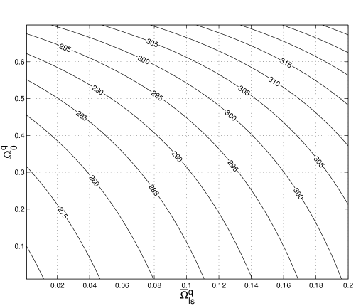
Figure 4: Contours of equal peak spacing $\Delta l$ as a function of $\Omega_{0}^{\phi}$ and ${\overline{\Omega}_{\rm ls}^{\phi}}$.The average equation of state is kept fixed, $\overline{w}_{0}=-0.7$. Increasing ${\overline{\Omega}_{\rm ls}^{\phi}}$ leads to a pronounced stretching of the spacing.

For fixed $\overline{w}_{0}$ and $\Omega_{0}^{\phi}$, we see from Equation (3) that $\Delta l\propto(1-{\overline{\Omega}_{\rm ls}^{\phi}})^{(-1/2)}$. Hence, when combining bounds on $\Omega_{0}^{\phi}$ and $\overline{w}_{0}$ from the structure of the Universe, supernovae redshifts and other sources with CMB data, the amount of dark energy in a redshift range of $z\sim 10^{5}$ to last scattering $z\sim 1100$ may be determined.

From Figure 2, we see that the averaged equation of state of the quintessence field for the present epoch is, in principle, a very influential quantity in determining the spreading of the peaks. Since combined large scale structure, supernovae and CMB analysis in (Bond et al., 2000) suggest $\overline{w}_{0}\lower 3.01385pt\hbox{$\;\stackrel{{\scriptstyle\textstyle<}}{{\sim}}\;$}-0.7$, the difference between a cosmological constant and quintessence may be hard to spot if ${\overline{\Omega}_{\rm ls}^{\phi}}$ is negligible. However, even with the data currently available, the first peak is determined to be at $l=212\pm 7$ (Bond et al., 2000). Once the third and fourth peak have been measured, the measurement of the spacing between the peaks becomes an averaging process with high precision. We can then hope to distinguish between different scenarios.

6 Conclusions

The influence of quintessence on the spacing between the CMB peaks is determined by three quantities: $\Omega_{0}^{\phi}$, $\overline{\Omega}_{\rm ls}^{\phi}$, and $\overline{w}_{0}$. When the location of the third peak is accurately measured, we can hope to be able to discriminate between a pure cosmological constant and a form of dark energy that has a non-trivial equation of state – possibly, and most likely, changing in time. The peak ratios will help determining $\overline{\Omega}_{\rm ls}^{\phi}$ which in principle can also be extracted from $\Delta l$, if $\Omega_{0}^{\phi}$ and $\overline{w}_{0}$ are measured by independent observations. With $\overline{\Omega}_{\rm ls}^{\phi}$ fixed, the peak spacing can be used to constrain $\Omega_{0}^{\phi}$ and $\overline{w}_{0}$. This can permit consistency checks for the quintessence scenario. Together with bounds on $\Omega^{\phi}$ for the period of structure formation ($5\lower 3.01385pt\hbox{$\;\stackrel{{\scriptstyle\textstyle<}}{{\sim}}\;$}z\lower 3.01385pt\hbox{$\;\stackrel{{\scriptstyle\textstyle<}}{{\sim}}\;$}10^{4}$) and the bound $\Omega_{BBN}^{\phi}<0.2$ from big bang nucleosynthesis (Wetterich, 1988, 1995; Birkel & Sarkar, 1997) ($z\sim 10^{9}$) we will post a few milestones in our attempt to trace the cosmological history of quintessence.

Table 1: Location and spacing of the CMB peaks for several models

${\overline{\Omega}_{\rm ls}^{\phi}}$	$\overline{w}_{0}$	$l_{1}$	$l_{2}$	$l_{2}/l_{1}$	$\Delta l^{\rm estim.}$	$\Delta l^{\rm num.}$	$\sigma_{8}$
Leaping kinetic term (A), $\Omega_{0}^{\phi}=0.6$
$8.4\times 10^{-3}$	$-0.76$	$215$	$518$	$2.41$	$292$	$291$	$0.86$
$0.03$	$-0.69$	$214$	$520$	$2.43$	$294$	$293$	$0.78$
$0.13$	$-0.45$	$211$	$523$	$2.48$	$299$	$300$	$0.47$
$0.22$	$-0.32$	$207$	$524$	$2.53$	$302$	$307$	$0.29$
Inverse power law potential (B), $\Omega_{0}^{\phi}=0.6$
$8.4\times 10^{-8}$	$-0.37$	$199$	$480$	$2.41$	$271$	$269$	$0.61$
$9.9\times 10^{-2}$	$-0.13$	$178$	$443$	$2.49$	$252$	$252$	$0.18$
$0.22$	$-8.1\times 10^{-2}$	$172$	$444$	$2.58$	$257$	$257$	$0.09$
Pure exponential potential, $\Omega_{0}^{\phi}=0.6$
$0.70$	$7\times 10^{-3}$	$190$	$573$	$3.02$	$368$	$377$	$0.01$
Pure exponential potential, $\Omega_{0}^{\phi}=0.2$
$0.22$	$4.7\times 10^{-3}$	$194$	$490$	$2.53$	$282$	$281$	$0.38$
Cosmological constant (C), $\Omega_{0}^{\phi}=0.6$
$0$	$-1$	$219$	$527$	$2.41$	$296$	$295$	$0.97$
Cold Dark Matter - no dark energy, $\Omega_{0}^{\phi}$ = 0
$0$	$\cdots$	$205$	$496$	$2.42$	$269$	$268$	$1.49$

Table 2: Horizons in Mpc at last scattering and today for various kinds of quintessence.

${\overline{\Omega}_{\rm ls}^{\phi}}$	$w_{0}$	$\overline{w}_{0}$	$\tau_{0}^{\rm estim.}$	$\tau_{0}^{\rm num.}$	$\Delta\tau_{0}$	$\tau_{\rm ls}^{\rm estim.}$	$\Delta\tau_{\rm ls}$
Leaping kinetic term (A), $\Omega_{0}^{\phi}=0.6$
$8.4\times 10^{-3}$	$-0.79$	$-0.76$	$13073$	$13060$	$0.1\%$	$266$	$0.3\%$
$0.03$	$-0.79$	$-0.69$	$12971$	$13000$	$0.2\%$	$263$	$0.3\%$
$0.13$	$-0.78$	$-0.45$	$12470$	$12590$	$1.0\%$	$248$	$0.2\%$
$0.22$	$-0.75$	$-0.32$	$12012$	$12175$	$1.3\%$	$236$	$0.0\%$
Inverse power law potential (B), $\Omega_{0}^{\phi}=0.6$
$8.4\times 10^{-8}$	$-0.32$	$-0.37$	$12205$	$12147$	$0.5\%$	$267$	$0.0\%$
$9.9\times 10^{-2}$	$-0.16$	$-0.13$	$10774$	$10798$	$0.2\%$	$253$	$0.2\%$
$0.22$	$-0.1$	$-8.1\times 10^{-2}$	$10241$	$10273$	$0.3\%$	$236$	$0.2\%$
Pure exponential potential, $\Omega_{0}^{\phi}=0.6$
$0.70$	$0.00$	$7\times 10^{-3}$	$9014$	$9049$	$0.4\%$	$146$	$2.3\%$
Pure exponential potential, $\Omega_{0}^{\phi}=0.2$
$0.22$	$5\times 10^{-5}$	$4.7\times 10^{-3}$	$9107$	$9120$	$0.1\%$	$191$	$0.3\%$
Cosmological constant (C), $\Omega_{0}^{\phi}$ = 0.6
$0$	$-1$	$-1$	$13330$	$13325$	$0.0\%$	$267$	$0.0\%$
Cold Dark Matter - no dark energy, $\Omega_{0}^{\phi}$ = 0
$0$	$\cdots$	$\cdots$	$9133$	$9133$	$0.0\%$	$201$	$0.5\%$

Table 3: Symbols, their meanings and numerical values used in this paper.

Symbol	Meaning	Value
$M_{\bar{P}}$	reduced Planck mass $M_{\bar{P}}^{-2}\equiv 8\pi G$	$\cdots$
$a(\tau)$	scale factor, normalised to unity today	$\cdots$
$a_{\rm ls}$	scale factor at last scattering	$1100^{-1}$
$h_{0}$	Hubble parameter today $H_{0}=100\,h_{0}\,\textrm{km s}^{-1}{\rm Mpc}^{-1}$	$0.65$
$\Omega_{0}^{\rm r}$	relativistic $\Omega$ today	$9.89\times 10^{-5}$
$\Omega_{0}^{\rm b}$	baryon $\Omega$ today	$0.05$
$\bar{c}_{s}$	$\tau$-averaged sound speed until last scattering	$0.52$
$n$	spectral index of initial perturbations	$1$

References

- Amendola (2000) Amendola, L., MNRAS, 312, 521
- de Bernadis et al. (2000) de Bernardis, P. et al. 2000, Nature, 404, 955
- Birkel & Sarkar (1997) Birkel, M., & Sarkar, S. 1997, Astropart. Phys., 6, 197
- Bond et al. (2000) Bond, J. R. et al. 2000, preprint (astro-ph/0011379)
- Brax et al. (2000) Brax, P., Martin, J., & Riazuelo, A. 2000, Phys. Rev. D, 62, 103505
- Caldwell et al. (1998) Caldwell, R. R., Dave, R., & Steinhardt, P. J. 1998, Phys. Rev. Lett., 80, 1852
- Coble et al. (1997) Coble, K., Dodelson, S., & Frieman, J. 1997, Phys. Rev. D, 55, 1851
- Doran & Lilley (2001) Doran, M., and Lilley, M., in preparation
- Efstathiou (1999) Efstathiou, G. 1999, preprint (astro-ph/9904356)
- Ferreira & Joyce (1997) Ferreira, P. G., & Joyce, M. 1997, Phys. Rev. Lett., 79, 4740
- Ferreira & Joyce (1998) Ferreira, P. G., & Joyce, M. 1998, Phys. Rev. D, 58, 023503
- Hanany et al. (2000) Hanany, S. et al. 2000, ApJ, 545, L5
- Hebecker & Wetterich (2000) Hebecker, A., & Wetterich, C. 2000, Phys. Lett. B, 497, 281
- Hu et al. (2000) Hu, W., Fukugita, M., Zaldarriaga, M., & Tegmark, M., preprint (astro-ph/0006436)
- Hu & Sugiyama (1995) Hu, W., & Sugiyama, N. 1995, ApJ, 444, 489
- Hu et al. (1997) Hu, W., Sugiyama, N, & Silk. J 1997, Nature, 386, 37
- Huey et al. (1999) Huey, G., Wang, L., Dave, R., Caldwell, R. R., & Steinhardt, P. J. 1999, Phys. Rev. D, 59, 063005
- Peebles & Ratra (1988) Peebles, P. J. E., & Ratra, B. 1988, ApJ, 325, L17
- Ratra & Peebles (1988) Ratra, B., & Peebles, P. J. E. 1988, Phys. Rev. D, 37, 3404
- Seljak & Zaldarriaga (1996) Seljak, U., & Zaldarriaga, M. 1996, ApJ, 469, 437
- Wetterich (1988) Wetterich, C. 1988, Nucl. Phys. B, 302, 668
- Wetterich (1995) Wetterich, C. 1995, A&A, 301, 321