Dynamical variations of the differential rotation in the solar convection zone

Abstract

Recent analyses of helioseismological observations seem to suggest the presence of two new phenomena connected with the dynamics of the solar convective zone. Firstly, there are present torsional oscillations with periods of about 11 years, which penetrate significantly into the solar convection zone and secondly, oscillatory regimes exist near the base of the convection which are markedly different from those observed near the top, having either significantly reduced periods or being non-periodic.

Recently spatiotemporal fragmentation / bifurcation has been proposed as a possible dynamical mechanism to account for such observed multi-mode behaviours in different parts of the solar convection zone. Evidence for this scenario was produced in the context of an axisymmetric mean field dynamo model operating in a spherical shell, with a semi–open outer boundary condition and a zero order angular velocity obtained by the inversion of the MDI data, in which the only nonlinearity was the action of the Lorentz force of the dynamo generated magnetic field on the solar angular velocity.

Here we make a detailed study of the robustness of this model with respect to plausible changes to its main ingredients, including changes to the $\alpha$ and $\eta$ profiles as well as the inclusion of a nonlinear $\alpha$ quenching. We find that spatiotemporal fragmentation is present in this model for different choices of the rotation data and as the details of the model are varied. Taken together, these results give strong support to the idea that spatiotemporal fragmentation is likely to occur in general dynamo settings.

1 Introduction

Recent analyses of the helioseismological data, from both the Michelson Doppler Imager (MDI) instrument on board the SOHO spacecraft (Howe et al. 2000a) and the Global Oscillation Network Group (GONG) project (Antia & Basu 2000) have provided strong evidence to indicate that the previously observed time variation of the differential rotation on the solar surface – the so called ‘torsional oscillations’ with periods of about 11 years (e.g. Howard & LaBonte 1980; Snodgrass, Howard & Webster 1985; Kosovichev & Schou 1997; Schou et al. 1998) – penetrates into the convection zone, to a depth of at least 9 percent of the solar radius. Torsional oscillations are thought to be a consequence of the nonlinear interactions between the magnetic fields and the solar differential rotation. A number of attempts have been made to model these oscillations. These include modelling the dynamical feedback of the large scale magnetic field on the turbulent Reynolds stresses that generate the differential rotation in the convection zone (the ‘nonlinear $\Lambda$–effect’: Kitchatinov 1988; Rüdiger & Kitchatinov 1990; Kitchatinov et al. 1994; Küker et al. 1996; Kitchatinov & Pipin 1998; Kitchatinov et al. 1999), as well as models in which the nonlinearity is through the direct action of the azimuthal component of the Lorentz force of the dynamo generated magnetic field on the solar angular velocity (e.g. Schuessler 1981; Yoshimura 1981; Brandenburg & Tuominen 1988; Jennings 1993; Covas et al. 2000a,b; Durney 2000).

Further studies of these data have produced intriguing, but rather contradictory results. Howe et al. (2000b) find evidence for the presence of such oscillations around the tachocline near the bottom of the convection zone, but with markedly shorter periods of about $1.3$ years. On the other hand, Antia & Basu (2000) do not find such oscillations at the bottom of the convective zone. Whatever the true dynamical behaviour at these lower levels may be, the crucial point about these recent results is that they both seem to indicate the possibility that the variations in the differential rotation can have different dynamical modes of behaviour at different depths in the solar convection zone: oscillations with a very different period in the former case and non-periodic behaviour in the latter.

Clearly, further observations are required to clarify this situation. However, whatever the outcome of such observations, it is of interest to ask whether such different variations can in principle occur in different spatial locations in the convection zone and, if so, what could be the possible mechanism(s) for their production. This is of particular interest given the inevitable errors in helioseismological inversions, especially as depth increases.

Recently, spatiotemporal fragmentation/bifurcation has been proposed as a possible dynamical mechanism to account for the observed multi-mode behaviour at different parts of the solar convection zone (Covas et al. 2000b) (hereafter CTM). This occurs when dynamical regimes which possess different temporal behaviours coexist at different spatial locations, at given values of the control parameters of the system. The crucial point is that these different dynamical modes of behaviour can occur without requiring changes in the parameters of the model, in contrast to the usual temporal bifurcations which result in identical temporal behaviour at each spatial point, and which occur subsequent to changes in the model parameters. Also, as we shall see below, spatiotemporal fragmentation/bifurcation is a dynamical mechanism, the occurrence of which does not depend upon the detailed physics at different spatial locations.

Evidence for the occurrence of this mechanism was produced in CTM in the context of a two dimensional axisymmetric mean field dynamo model operating in a spherical shell, with a semi–open outer boundary condition, in which the only nonlinearity is the action of the azimuthal component of the Lorentz force of the dynamo generated magnetic field on the solar angular velocity. The zero order angular velocity was chosen to be consistent with the most recent helioseismological (MDI) data. Despite the success of this model in producing spatiotemporal fragmentation, a number of important questions remain. Firstly, there are error bars due to the nature of the observational data as well as inversion schemes used. Secondly, the model used by CTM is approximate and includes many simplifying assumptions. As a result, to be certain that spatiotemporal fragmentation can in fact be produced as a result of such nonlinear interactions, independently of the details of the model employed, it is necessary that it is robust, i.e. that it can produce such behaviour independently of these details.

The aims of this paper are twofold. Firstly, we make a systematic study of of this mechanism by making a comparison of the cases where the zero order rotational velocity are given by the inversions of the MDI and GONG data respectively. Given the detailed differences between these rotation profiles, this amounts to studying the robustness of the mechanism with respect to small changes in the zero order rotation profile.

Secondly, we study the robustness of this model (in producing spatiotemporal fragmentation) with respect to a number of plausible changes to its main ingredients, and demonstrate that the occurrence of this mechanism is not dependent upon the details of our model.

We show that in addition to producing butterfly diagrams which are in qualitative agreement with the observations as well as displaying torsional oscillations that penetrate into the convection zone, as recently observed by Howe et al. (2000a) and Antia & Basu (2000), and studied by Covas et al. (2000a), the model can produce qualitatively different forms of spatiotemporal fragmentary behaviours, which could in principle account for either of the contradictory types of dynamical behaviour observed by Howe et al. (2000b) and Antia & Basu (2000) at the bottom of the convection zone.

The structure of the paper is as follows. In the next section we outline our model. Section 3 contains our detailed results for both MDI and GONG data. In section 4 we study the robustness of spatiotemporal fragmentation with respect to various changes in the details of our model and finally section 5 contains our conclusions.

2 The model

We shall assume that the gross features of the large scale solar magnetic field can be described by a mean field dynamo model, with the standard equation

$$\frac{\partial{\bf B}}{\partial t}=\nabla\times({\bf u}\times{\bf B}+\alpha{\bf B}-\eta\nabla\times{\bf B}),$$ (1)

where $\@vec{B}$ and $\@vec{u}$ are the mean magnetic field and the mean velocity respectively. The quantities $\alpha$ (the $\alpha$ effect) and the turbulent magnetic diffusivity $\eta_{t}$, appear in the process of the parameterisation of the second order correlations between the velocity and magnetic field fluctuations ($\@vec{u}^{\prime}$ and $\@vec{B}^{\prime}$). Here ${\bf u}=v\mathbf{\hat{\@vec{\phi}}}-\frac{1}{2}\nabla\eta$, the term proportional to $\nabla\eta$ represents the effects of turbulent diamagnetism, and the velocity field is taken to be of the form $v=v_{0}+v^{\prime}$, where $v_{0}=\Omega_{0}r\sin\theta$, $\Omega_{0}$ is a prescribed underlying rotation law and the component $v^{\prime}$ satisfies

$$\frac{\partial v^{\prime}}{\partial t}=\frac{(\nabla\times{\bf B})\times{\bf B}}{\mu_{0}\rho r\sin\theta}.\mathbf{\hat{\@vec{\phi}}}+\nu D^{2}v^{\prime},$$ (2)

where $D^{2}$ is the operator $\frac{\partial^{2}}{\partial r^{2}}+\frac{2}{r}\frac{\partial}{\partial r}+\frac{1}{r^{2}\sin\theta}(\frac{\partial}{\partial\theta}(\sin\theta\frac{\partial}{\partial\theta})-\frac{1}{\sin\theta})$ and $\mu_{0}$ is the induction constant. The assumption of axisymmetry allows the field ${\bf B}$ to be split simply into toroidal and poloidal parts, ${\bf B}={\bf B}_{T}+{\bf B}_{P}=B\hat{\@vec{\phi}}+\nabla\times A\hat{\@vec{\phi}}$, and Eq. (1) then yields two scalar equations for $A$ and $B$. Nondimensionalizing in terms of the solar radius $R$ and time $R^{2}/\eta_{0}$, where $\eta_{0}$ is the maximum value of $\eta$, and putting $\Omega=\Omega^{*}\tilde{\Omega}$, $\alpha=\alpha_{0}\tilde{\alpha}$, $\eta=\eta_{0}\tilde{\eta}$, ${\bf B}=B_{0}\tilde{\bf B}$ and $v^{\prime}=\Omega^{*}R\tilde{v}^{\prime}$, results in a system of equations for $A,B$

$$\frac{\partial A}{\partial\tau} = w_{r}B_{\theta}-w_{\theta}B_{r}+R_{\alpha}\tilde{\alpha}B+\tilde{\eta}D^{2}A,$$ (3)

$$\frac{\partial B}{\partial\tau} = R_{\omega}r\sin\theta{\bf B}.\nabla\Omega-\frac{1}{r}\frac{\partial}{\partial r}(rw_{r}B)$$

$$- \frac{1}{r}\frac{\partial}{\partial\theta}(w_{\theta}B)+\frac{1}{r^{2}\sin\theta}\frac{\partial\tilde{\eta}}{\partial\theta}(B\sin\theta)$$

$$+ R_{\alpha}\left(-\tilde{\alpha}D^{2}\alpha+\frac{\partial\tilde{\alpha}}{\partial r}B_{\phi}-\frac{1}{r}\frac{\partial\tilde{\alpha}}{\partial\theta}B_{r}\right)$$

$$+ \frac{1}{r}\frac{\partial\tilde{\eta}}{\partial r}\frac{\partial}{\partial r}(rB)+\tilde{\eta}D^{2}B,$$

where ${\bf w}=-\frac{1}{2}\nabla\eta$. The dynamo parameters are $R_{\alpha}=\alpha_{0}R/\eta_{0}$, $R_{\omega}=\Omega^{*}R^{2}/\eta_{0}$, $P_{r}=\nu_{0}/\eta_{0}$, and $\tilde{\eta}=\eta/\eta_{0}$, where $\Omega^{*}$ is the solar surface equatorial angular velocity. Here $\nu_{0}$ and $\eta_{0}$ are the values of the turbulent magnetic diffusivity and viscosity respectively and $P_{r}$ is the turbulent Prandtl number. The density $\rho$ is assumed to be uniform.

For our inner boundary conditions we chose $B=0$ on $r=r_{0}$ (which enforces angular momentum conservation in the dynamo region, as discussed in Moss & Brooke 2000). At the outer boundary, we used an open boundary condition $\partial B/\partial r=0$ on $B$, and vacuum boundary conditions for ${\bf B}_{P}$ (as in CTM). The motivation for the former condition is that the surface boundary condition is ill-defined, and there is some evidence that the more usual $B=0$ condition may be inadequate. This issue has recently been discussed at length by Kitchatinov, Mazur & Jardine (2000), who derive ‘non-vacuum’ boundary conditions on both $B$ and ${\bf B}_{P}$.

Equations (2), (3) and (2) were solved using the code described in Moss & Brooke (2000) (see also Covas et al. 2000a,b) together with the above boundary conditions, over the range $r_{0}\leq r\leq 1$, $0\leq\theta\leq\pi$. We set $r_{0}=0.64$; with the solar convection zone proper being thought to occupy the region $r\;\raise 1.29167pt\hbox{$>$\kern-7.5pt\raise-4.73611pt\hbox{$\sim$ }}\;\hskip-2.0pt0.7$, the region $r_{0}\leq r\;\raise 1.29167pt\hbox{$<$\kern-7.5pt\raise-4.73611pt\hbox{$\sim$ }}\;\hskip-2.0pt0.7$ can be thought of as an overshoot region/tachocline. In the following simulations we used a mesh resolution of $61\times 101$ points, uniformly distributed in radius and latitude respectively.

The model employed in CTM had the following ingredients. In the interval $0.64\leq r\leq 1$, $\Omega_{0}$ was given by the inversion of the MDI data obtained from 1996 to 1999 by Howe et al. (2000a). Here, in addition to this, we shall for comparison also use the $\Omega_{0}$ given by the inversion of the GONG data obtained from 1995 to 1999 by Howe et al. (2000b). The form of $\alpha$ was taken as

$$\tilde{\alpha}=\alpha_{r}(r)f(\theta),$$ (5)

where $f(\theta)=\sin^{4}\theta\cos\theta$ (cf. Rüdiger & Brandenburg 1995). The model possessed radial dependence in both $\alpha$ and the turbulent diffusion coefficient $\eta$: the $\alpha$ profile was chosen by setting $\alpha_{r}=1$ for $0.7\leq r\leq 0.8$ with cubic interpolation to zero at $r=r_{0}$ and $r=1$, with the convention that $\alpha_{r}>0$ and $R_{\alpha}<0$. The $\eta$ profile was chosen in order to take into account the likely decrease of $\eta$ in the overshoot region, by allowing a simple linear decrease in $\tilde{\eta}$ from $\tilde{\eta}=1$ at $r=0.8$ to $\tilde{\eta}=0.5$ in $r<0.7$.

In the following sections we shall, in addition to these particular profiles, also consider variations to them in order to study the robustness of the model (in producing spatiotemporal fragmentation) with respect to such changes. Also for the sake of comparison, we shall use the interpolation on the GONG data for the rotation law as well as allowing other changes.

3 Torsional oscillations and fragmentation using the MDI and GONG data sets

In this section, we study the presence of spatiotemporal fragmentation and torsional oscillations, using the zero order angular velocity obtained by the inversion of the GONG data (see Fig. 1). This allows a detailed comparison to be made with the results of CTM which employed the corresponding MDI data (see Fig. 2), including the magnetic field structure and strengths as well as the nature of torsional oscillations, as a function of depth and latitude.

Figure 1: Isolines of the time average of the angular velocity of the solar rotation, obtained by inversion techniques using the GONG data (Howe et al. 2000b). Contours are labelled in units of nHz.

Figure 2: Isolines of the time average of the angular velocity of the solar rotation, obtained by inversion techniques from the MDI data (Howe et al. 2000a). Contours are labelled in units of nHz.

To begin with, we calibrated our model in each case so that near marginal excitation the cycle period was about 22 years. This determined $R_{\omega}$ to be $44000$, corresponding to $\eta_{0}\approx 3.4\times 10^{11}$ cm² sec^-1, given the known values of $\Omega^{*}$ and $R$.

In both cases, the first solutions to be excited in the linear theory are limit cycles with odd (dipolar) parity with respect to the equator, with marginal dynamo numbers $R_{\alpha}\approx-3.05$ and $-3.11$ respectively for the GONG and MDI data. The even parity (quadrupolar) solutions are also excited at similar marginal dynamo numbers of $R_{\alpha}\approx-3.20$ and $-3.22$, respectively. We note that these marginal dynamo numbers are slightly different from those reported in CTM as we have used here $f(\theta)=\sin^{4}\theta\cos\theta$ for the $\theta$–dependence of the $\alpha$ effect, whilst CTM used the prescription $f(\theta)=\sin^{2}\theta\cos\theta$.

Also, to be consistent with CTM, we chose the value of the Prandtl number in this section to be $P_{r}=1.0$. For the parameter range that we investigated, the even parity solutions can be nonlinearly stable. Given that the Sun is observed to be close to an odd (dipolar) parity state, and that previous experience shows that small changes in the physical model can cause a change between odd and even parities in the stable nonlinear solution, we chose to impose dipolar parity on our solutions, effectively solving the equations in one quadrant, $0\leq\theta\leq\pi/2$, and imposing appropriate boundary conditions at the equator $\theta=\pi/2$.

With these parameter values, we found that this model, with the underlying zero order angular velocity chosen to be consistent with either the MDI or the GONG data, is capable of producing butterfly diagrams which are in qualitative agreement with the observations, as can be seen in Figs. 3 and 4. We note that the butterfly diagrams in the GONG case tend to be smoother and to have weaker polar branches, presumably because the MDI inversion is respectively less smooth and has a distinctive polar jet close to $r=0.95R_{\odot}$.

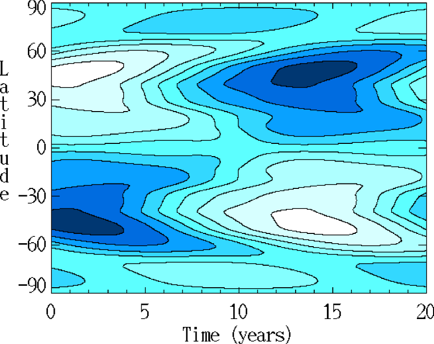
Figure 3: Butterfly diagram of the toroidal component of the magnetic field $\@vec{B}$ at fractional radius $r=0.95$ for the MDI data. Dark and light shades correspond to positive and negative values of $B_{\phi}$ respectively. Parameter values are $R_{\alpha}=-11.0$, $P_{r}=1.0$ and ${R_{\omega}}=44000$.

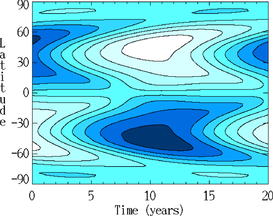
Figure 4: Butterfly diagram of the toroidal component of the magnetic field $\@vec{B}$ at fractional radius $r=0.95$ for the GONG data. Dark and light shades correspond to positive and negative values of $B_{\phi}$ respectively. Parameter values are $R_{\alpha}=-9.0$, $P_{r}=1.0$ and ${R_{\omega}}=44000$.

The model can also produce torsional oscillations in both cases (see Figs. 5 and 6), that penetrate into the convection zone, in a manner similar to those deduced from recent helioseismological data (Howe et al. 2000a; Antia & Basu 2000) and studied in Covas et al. (2000a,b).

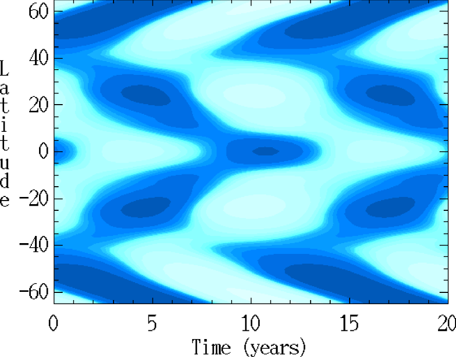
Figure 5: Variation of the perturbation to the zero order rotation rate in latitude and time, revealing the migrating banded zonal flows, taken at fractional radius $r=0.95$, with the MDI data. Parameter values are as in Fig. 3

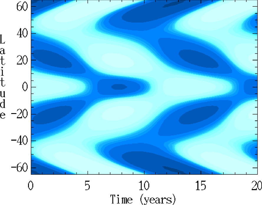
Figure 6: Variation of the perturbation to the zero order rotation rate in latitude and time, revealing the migrating banded zonal flows, taken at fractional radius $r=0.95$ with the GONG data. Parameter values are as in Fig. 4.

We also found the model to be capable of producing spatiotemporal fragmentation near the base of the convection zone, i.e. we found there different dynamical modes of behaviour in the differential rotation, including oscillations with reduced periods, as well as non-periodic variations as in CTM. These coexist with the near-surface torsional oscillations of the form shown in Figs. 5 and 6). To demonstrate this, we have plotted in Figs. 7 and 8 the radial contours of the angular velocity residuals $\delta\Omega$ as a function of time for a cut at latitude $30^{\circ}$. To demonstrate the period halving produced by the fragmentation more clearly, we have also plotted in Fig. 9 the residuals $\delta\Omega$ at different values of $R_{\alpha}$.

We also find that, in all cases, torsional oscillations with the same period persist in all the regions above the fragmentation level as can, for example, be seen from Figs. 7 and 8. The butterfly diagrams for the toroidal magnetic field, on the other hand, keep the same period and qualitative form throughout the convection zone, including the spatial regions that experience fragmentation, as shown in Figs. 10 and 11. Thus the fragmentation in the angular velocity residuals do not seem to be present in the magnetic field. Fig. 11 shows clearly that the fragmentation only occurs in $\delta\Omega$ and that the magnetic field retains its typical 22 year cycle throughout the dynamo region.

We also made a detailed study of the magnetic field evolution and the magnitude of torsional oscillations in each case. Fig. 12 summarises the results of the average magnetic energy as a function of $R_{\alpha}$, for both the MDI and the GONG data, and demonstrates that both data sets produce almost the same average magnetic energy for a given $R_{\alpha}$. Similarly, we have plotted in Fig. 13, the maxima (of the absolute value) of the residuals of the differential rotation, $\delta\Omega$, as a function of $R_{\alpha}$, for both MDI and the GONG data, which shows that for large values of $|R_{\alpha}|$, the GONG data produce larger residuals.

We end this section by summarising the qualitative modes of spatiotemporal behaviour our detailed numerical results have produced, for both MDI and GONG data. Our results show that our model is capable of producing three qualitatively different spatiotemporal modes of behaviour: (i) regimes in which there is no deformation of the torsional oscillation bands in the ($r,t$) plane, and hence no changes in phase or period through the convection zone; (ii) regimes in which there is deformation in the oscillatory bands in the ($r,t$) plane, resulting in changes in the phase of the oscillations, but no changes in their period and (iii) regimes with spatiotemporal fragmentation, resulting in changes both in phase as well as in period/behaviour of oscillations. An example of the difference between such regions is given in Fig. 7, which shows a spatiotemporal fragmentation resulting in period halving, as well as a phase change between the oscillations near the surface and those deeper down in the convection zone. We should emphasise that by period we mean here the time between the maxima (minima), rather than time between repeated sequences. We note that given the presence of noise, the error bars induced by the inversion and the shortness of the observational interval, the time between the maxima (minima) is the most relevant quantity from the point of view of comparison with observations.

Our results also show that using the zero order rotation produced by both the MDI and GONG data gives rise to qualitatively similar results regarding both the spatiotemporal fragmentation and the torsional oscillations. There are, however, detailed quantitative differences. An example of this relates to the case (ii) above, where the location of where the fragmentation occurs is higher for MDI than for GONG at higher values of $|R_{\alpha}|$ (see Fig. 14). Furthermore, the phase shift is less pronounced for the MDI case than for the GONG case, specially at higher $|R_{\alpha}|$ values (see Fig. 15).

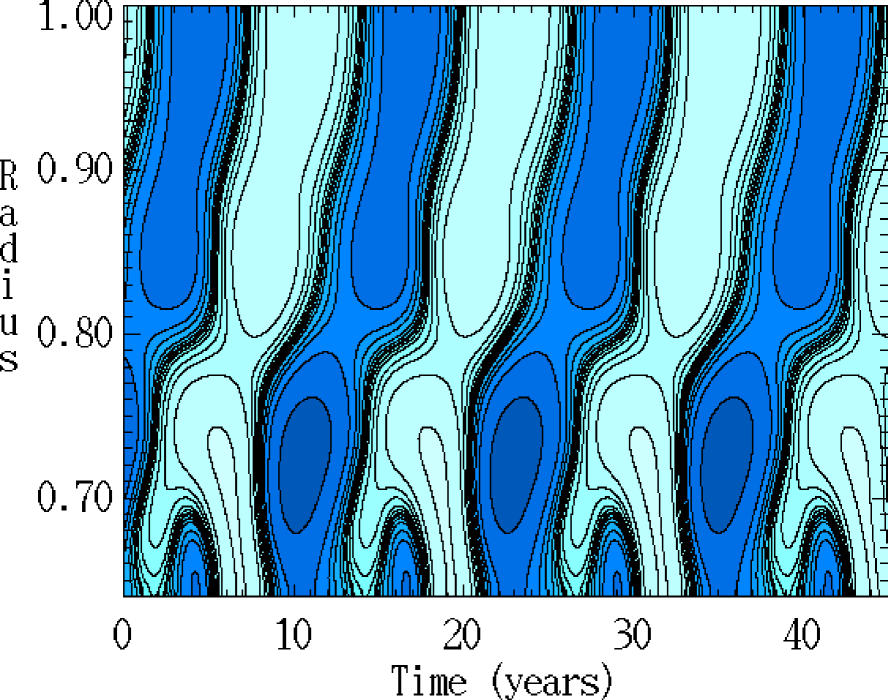
Figure 7: Radial contours of the angular velocity residuals $\delta\Omega$ as a function of time for a cut at latitude $30^{\circ}$, with the MDI data. Parameter values are as in Fig. 3.

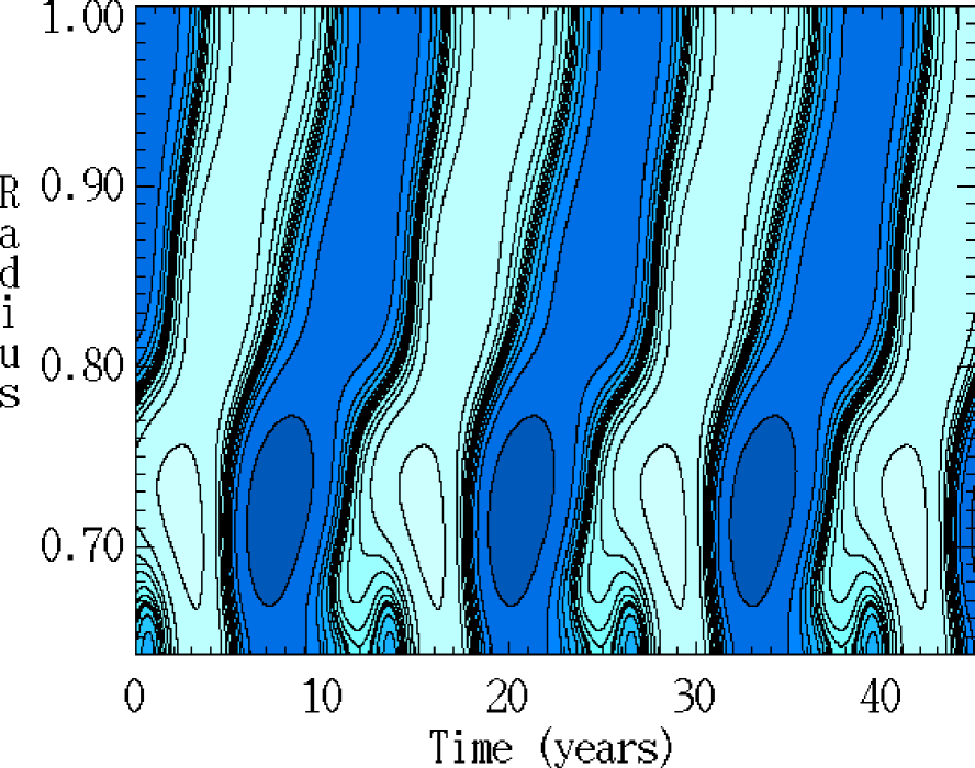
Figure 8: Radial contours of the angular velocity residuals $\delta\Omega$ as a function of time for a cut at latitude $30^{\circ}$, for the GONG data. Parameter values are as in Fig. 4.

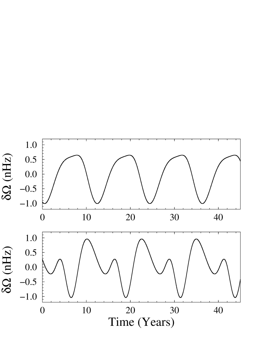
Figure 9: ‘Period halving’ at $r=0.68$ and latitude $30^{\circ}$. The panels correspond, from top to bottom, to $R_{\alpha}=-6.0$ and $-11.0$ respectively, and display increasing relative amplitudes of the secondary oscillations. The remaining parameter values are as in Fig. 3.

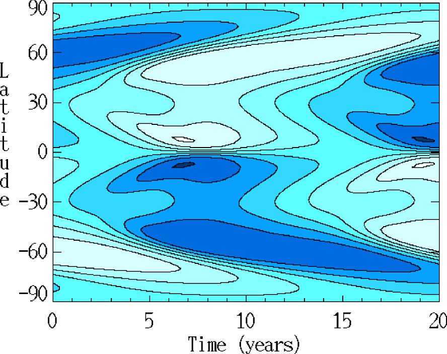
Figure 10: Butterfly diagram of the toroidal component of the magnetic field $\@vec{B}$ at fractional radius $r=0.68$ for the MDI data, showing no signs of fragmentation. Parameter values are as in Fig. 3.

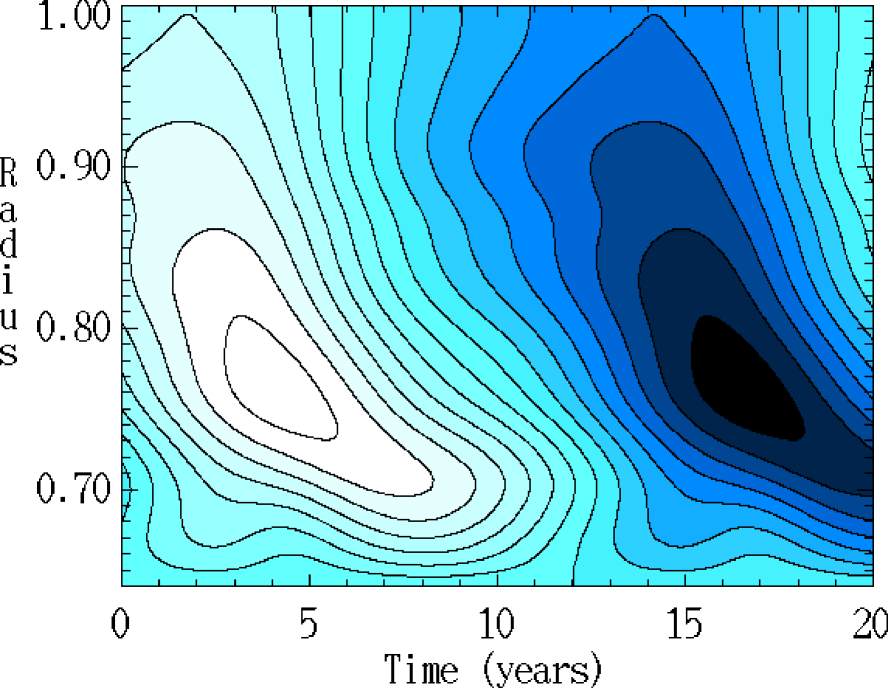
Figure 11: Radial contours of the toroidal component of the magnetic field $\@vec{B}$ as a function of time for a cut at latitude $30^{\circ}$, for the MDI data, showing no signs of fragmentation. This is the counterpart of the Fig. 8 and clearly shows that the fragmentation occurs only for $\delta\Omega(r,\theta,t)$ and that the magnetic field retains its typical 22 year cycle. Parameter values are as in Fig. 3.

Figure 12: The average magnetic energy $E_{M}$ as a function of $R_{\alpha}$, for both MDI and the GONG data. The parameter values are $P_{r}=1.0$ and ${R_{\omega}}=44000$.

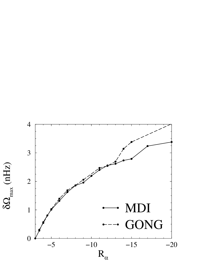
Figure 13: Comparison of the maximum of $\delta\Omega(r=0.95R_{\odot},\theta)$ for both the MDI and the GONG data sets. The parameter values are $P_{r}=1.0$ and ${R_{\omega}}=44000$.

Figure 14: Variation of fragmentation level (the maximum radius for which more than one fundamental period exists) as a function of the control parameter $R_{\alpha}$ for both the MDI and the GONG data sets. The parameter values are $P_{r}=1.0$ and ${R_{\omega}}=44000$.

Figure 15: Variation of phase shift $\phi$ as a function of the control parameter $R_{\alpha}$ for both the MDI and the GONG data sets. The phase shift evaluated by comparing the residual time series $\delta\Omega(r=0.95R_{\odot},\theta=30^{\circ})$ and $\delta\Omega(r=0.75R_{\odot},\theta=30^{\circ})$. A positive phase shift $\phi$ indicates a forward shift of the torsional oscillation bands (top to bottom) and a negative phase shift an opposite one. The parameter values are $P_{r}=1.0$ and ${R_{\omega}}=44000$.

4 Robustness of the model

As noted above, the model of the solar dynamo used by CTM to demonstrate the presence of torsional oscillations and spatiotemporal fragmentation is inevitably approximate in nature and contains major simplifications and parameterizations. It is therefore important to ask to what extent the spatiotemporal fragmentation, as well as the qualitative features of torsional oscillations found in CTM, depend on the details of the model employed.

In order to go some way towards answering these questions, we shall in this section study the robustness of this model with respect to plausible changes to its main ingredients, considering these changes one by one.

A feature of the model considered by CTM is the presence of radial variations in both $\alpha$ and $\eta$, and in particular the fact that $\alpha$ was taken to be zero in $r\leq 0.70$. An obvious question is whether this variation is the source of the fragmentation described above, for example does it cause the dynamo region essentially to consist of two disparate parts, each with its own set of properties? This is perhaps unlikely, as there is no independent dynamo action in $r\leq 0.7$, as $\alpha=0$ there. Nevertheless, to resolve this issue, we study the effects of changes in the radial variations of both $\alpha$ and $\eta$ and subsequently examine a model in which neither vary radially.

Given the qualitative similarity of the results produced using the MDI and the GONG data, and in order to keep the extent of the computations within tractable bounds, we consider only the MDI data in the following sections.

4.1 Robustness with respect to changes in the $\alpha$ profile

We studied this by setting $\alpha_{r}=1$ throughout the computational region, which changes the $\alpha$ profile substantially. In spite of this, we found qualitatively similar forms of butterfly diagrams, torsional oscillations and spatiotemporal fragmentation in this case as in the case of CTM. An example of such fragmentation in the radial contours of $\delta\Omega$ is given in Fig. 16.

We note that the change in the $r$-dependence of $\alpha$ does not change the calibration of $R_{\omega}$ required to produce a cycle period of 22 years. It does, however, seem to change the details of the surface torsional oscillations, making them somewhat less realistic. It also, importantly from the point of view of observations, enhances the phase shift between the torsional oscillations at the top and below the deformation, to a phase change of $\phi=-\pi$ as can be seen from Fig. 27. Note, however, that the phase shift $\phi$ changes continuously with $R_{\alpha}$.

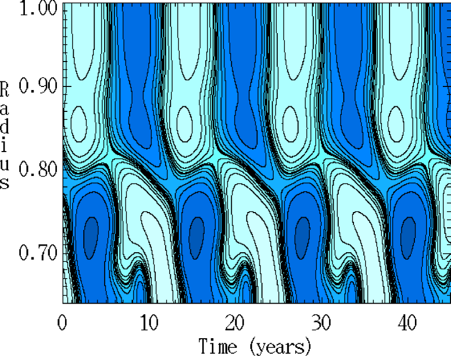
Figure 16: Radial contours of the angular velocity residuals $\delta\Omega$ as a function of time for a cut at latitude $30^{\circ}$. The parameter values are $R_{\omega}=44000$, $R_{\alpha}=-11.0$ and $Pr=1.0$ with $\alpha_{r}(r)=1$.

4.2 Robustness with respect to $\eta$ profile

To obtain some idea of the sensitivity of the model to the chosen radial dependence of the turbulent diffusion coefficient $\eta$, we then examined a model in which $\tilde{\eta}(r)=1$ throughout. In this way we removed from the model the inhomogeneity associated with $\eta$ at the base of the convection zone.

We found that with this form of $\eta$, $R_{\omega}$ needs to be recalibrated to $R_{\omega}=60000$ in order to produce toroidal field butterfly diagrams at the surface with a period of 22 years.

With this value of $R_{\omega}$, we again found qualitatively similar forms of spatiotemporal fragmentation in this case, to those obtained by CTM. An example is given in Fig. 17.

We note that, compared with the behaviour of the original model depicted in Figs. 4, this model produces more realistic torsional oscillations at the surface than the model with the radial dependence of $\alpha$ removed. However, the butterfly diagrams of the toroidal magnetic field near the surface look slightly less realistic than those for the original model shown in Fig. 3. But, it must be borne in mind that in the absence of a definitive sunspot model, it is not obvious at which depth the toroidal field patterns correspond to the observed butterfly diagram. Furthermore, as a result of the removal of the radial variation of $\eta$ in this model, the effective magnetic turbulent diffusivity changes and consequently the range of $R_{\alpha}$ values for spatiotemporal fragmentation are somewhat higher than for the model employed by CTM. We note also that the fragmentation is now present at higher radius and is in this case detached from the lower boundary.

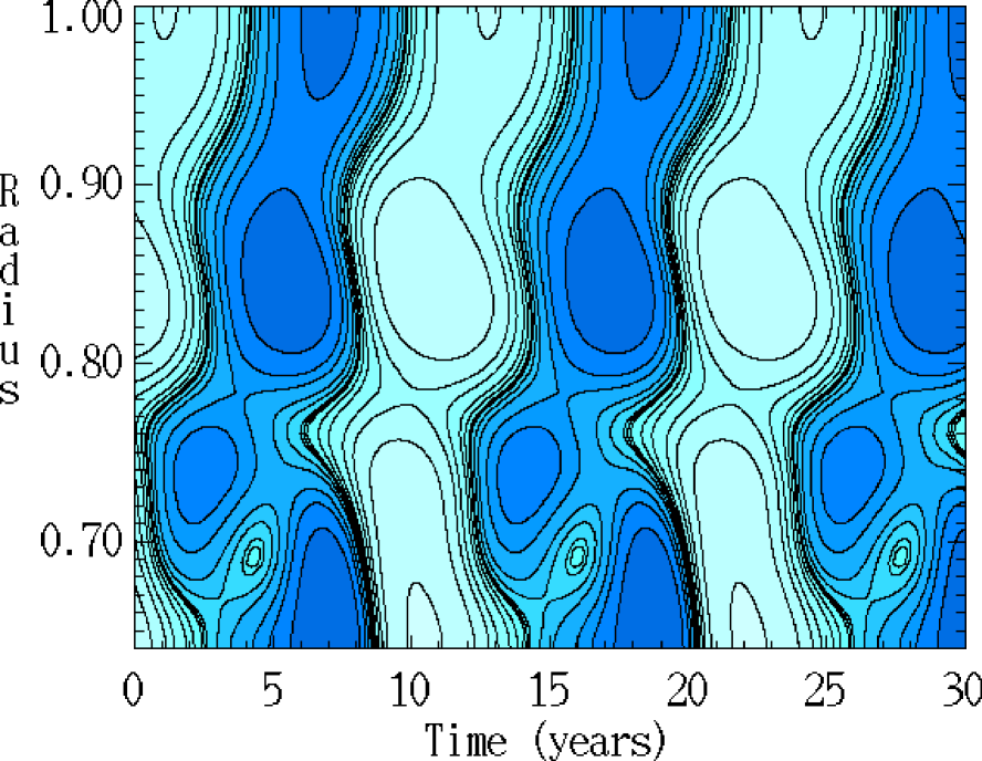
Figure 17: Radial contours of the angular velocity residuals $\delta\Omega$ as a function of time for a cut at latitude $30^{\circ}$. The parameter values are $R_{\omega}=60000$, $R_{\alpha}=-16.0$ and $Pr=1.0$ with $\tilde{\eta}(r)=1$.

4.3 Robustness to simultaneous removal of radial dependence of $\alpha$ and $\eta$

In the last two sections we studied the robustness of the spatiotemporal fragmentation and the torsional oscillations with respect to the removal of the radial dependence of $\alpha$ and $\eta$ in turn. Interestingly, in both cases we found the spatiotemporal fragmentation to persist. Here we investigate a model in which both $\alpha$ and $\eta$ are independent of radius, so that (unrealistically) the convective region and overshoot layer are only distinguished by the nature of the given zero order rotation law. Thus we considered a modification of the model considered by CTM, given by taking $\alpha_{r}=\tilde{\eta}(r)=1$. Perhaps surprisingly, we still found spatiotemporal fragmentation, as can be seen in Fig. 18.

We note, however, that in this case both the butterfly diagrams of the toroidal field and the torsional oscillations near the surface look less realistic than the original model of Sect. 3. Our point is however that spatiotemporal fragmentation appears to be a general property of the type of dynamo models studied, and is not crucially dependent on imposed spatial structures in the coefficients $\alpha$ and $\eta$, that might be thought to distinguish the lower part of the dynamo region from the subsurface layers. We also note that again the fragmentation region is detached from the lower boundary (suggesting that this is a feature related to the $\eta$ profile) and extends to an even greater height, $r=0.71R_{\odot}$. It is interesting that, within our limited experimentation, the details of the fragmentation, but not its existence, seem to be quite sensitive to the $\eta$ profile.

We also studied the average magnetic energy and the residuals, $\delta\Omega$, as a function of $R_{\alpha}$ with different $\alpha$ and $\eta$ profiles and these are depicted in Figs. 19 and 20. As can be seen, the values of $\delta\Omega$ are larger for the case with radial variations of both $\alpha$ and $\eta$ present, whereas the average magnetic energy is largest for the case with uniform $\eta$.

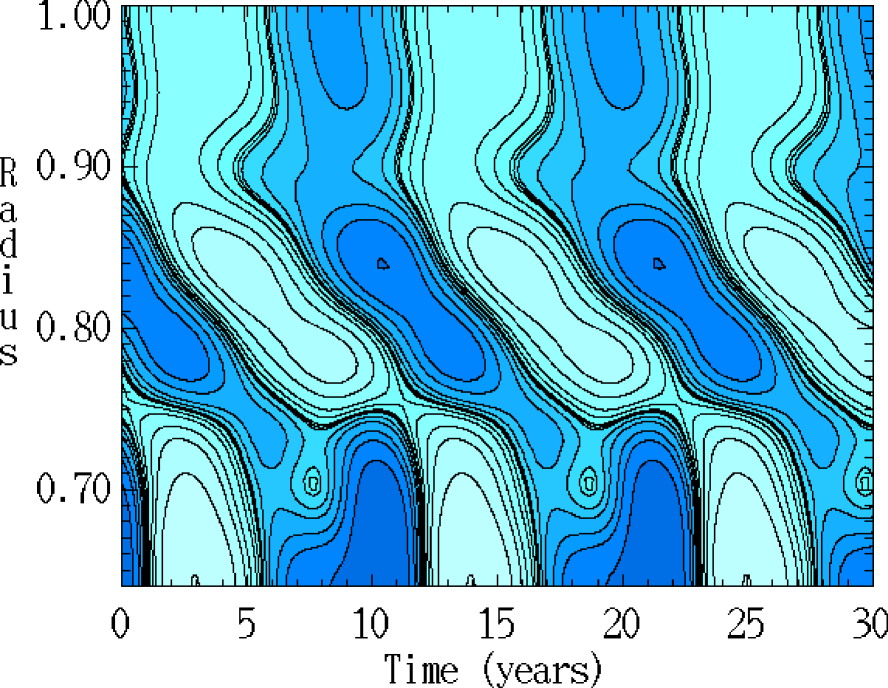
Figure 18: Radial contours of the angular velocity residuals $\delta\Omega$ as a function of time for a cut at latitude $30^{\circ}$. Parameter values are $R_{\omega}=60000$, $R_{\alpha}=-15.0$ and $Pr=1.0$ with $\eta(r,\theta)=1$ and $\alpha_{r}(r)=1$.

Figure 19: Comparison of the average magnetic energy $E_{M}$ as a function of $R_{\alpha}$ for models with different $\alpha$ profiles. The parameter values are $P_{r}=1.0$ and ${R_{\omega}}=44000$. The continuous curve represents the results of the model with $\alpha_{r}=f(r),\eta(r,\theta)=\eta(r)$, the long-dashed curve the model with $\alpha_{r}=1=\eta(r,\theta)$, the short-dashed curve the model with $\eta(r,\theta)=1$ and the dotted-dashed curve the model with $\alpha_{r}=1$.

Figure 20: Comparison of the maximum of $\delta\Omega(r=0.95R_{\odot},\theta)$ for models with different $\alpha$ profiles. The parameter values and the characterisation of the curves is as in Fig. 19.

4.4 Robustness with respect to $\alpha$ quenching

Even though the model used by CTM was nonlinear (via the Lorentz force and the subsequent $v^{\prime}$ term in the induction equation), the magnitude of $\alpha$ was fixed ab initio. We note that the form of $\alpha_{r}$ in the original model was initially chosen to represent implicit strong $\alpha$-quenching occurring in the overshoot layer, in that $\alpha=0$ in $r\leq 0.7$. In this section we study the effects of having an additional nonlinearity in the form of an $\alpha$ quenching given by

$$\tilde{\alpha}=\alpha_{r}(r)\frac{\sin^{4}\theta\cos\theta}{1+g|{\bf B}^{2}|}$$ (6)

where $g$ is a quenching factor, in addition to the nonlinearity given by Eq. (2).

In this connection it may be noted that there is an ongoing controversy regarding the nature and strength of $\alpha$-quenching. This is not the place to rehearse the arguments for and against ‘strong’ alpha-quenching; the issue is unresolved, and we use (6) as a commonly adopted nonlinearity.

We found that for values of $g\;\raise 1.29167pt\hbox{$<$\kern-7.5pt\raise-4.73611pt\hbox{$\sim$ }}\;\hskip-2.0pt0.1$ (depending somewhat on $R_{\alpha}$ and $P_{r}$), the model continues to produce torsional oscillations and spatiotemporal fragmentation.

4.5 Robustness with respect to the Prandtl number $P_{r}$

In the results obtained by CTM, the Prandtl number was taken as $P_{r}=1$. In this section we study the effects of changing $P_{r}$ on the nature of spatiotemporal fragmentation and torsional oscillations.

Our studies show that, for our model, both spatiotemporal fragmentation and torsional oscillations persist for values of Prandtl number given by $P_{r}\;\raise 1.29167pt\hbox{$>$\kern-7.5pt\raise-4.73611pt\hbox{$\sim$ }}\;\hskip-2.0pt0.4$ (depending on $R_{\alpha}$). Around $P_{r}\approx 0.4$, however, a sudden transition seems to occur, such that below this value spatiotemporal fragmentation as well as coherent surface torsional oscillations seem to be absent.

We also made a detailed study of the magnetic field strength as well as of the magnitude of the torsional oscillations, for different values of Prandtl number $P_{r}$. Figs. 21 and 22 show the behaviours of the average magnetic energy and the residuals of the differential rotation, $\delta\Omega$, for fixed $R_{\alpha}$, for different values of Prandtl number $P_{r}$. This is in agreement with the results of Küker et al. 1996, who studied solar torsional oscillations in a model with magnetic quenching of the Reynolds stresses (the ‘$\Lambda$-effect’), with both studies showing a linear growth of the amplitude of the torsional oscillations as a function of (small) Prandtl number. In their case the amplitudes of the torsional oscillations for $P_{r}\;\raise 1.29167pt\hbox{$<$\kern-7.5pt\raise-4.73611pt\hbox{$\sim$ }}\;\hskip-2.0pt1$ are weaker than observed, whereas in our model they are within physically more reasonable ranges, $\delta\Omega\approx 0.5$–$1$ nHz. However, the restriction to uniform density makes it uncertain how important these amplitude differences really are.

Finally we also studied the average magnetic energy and the maximum value of the residuals, $\delta\Omega$, as a function of $R_{\alpha}$ for a number of cases, including a nonlinearly quenched $\alpha$, as shown in Figs. 23 and 24. The decrease in $P_{r}$ results in the reduction of the average magnetic energy and the residuals, as can be seen from these figures.

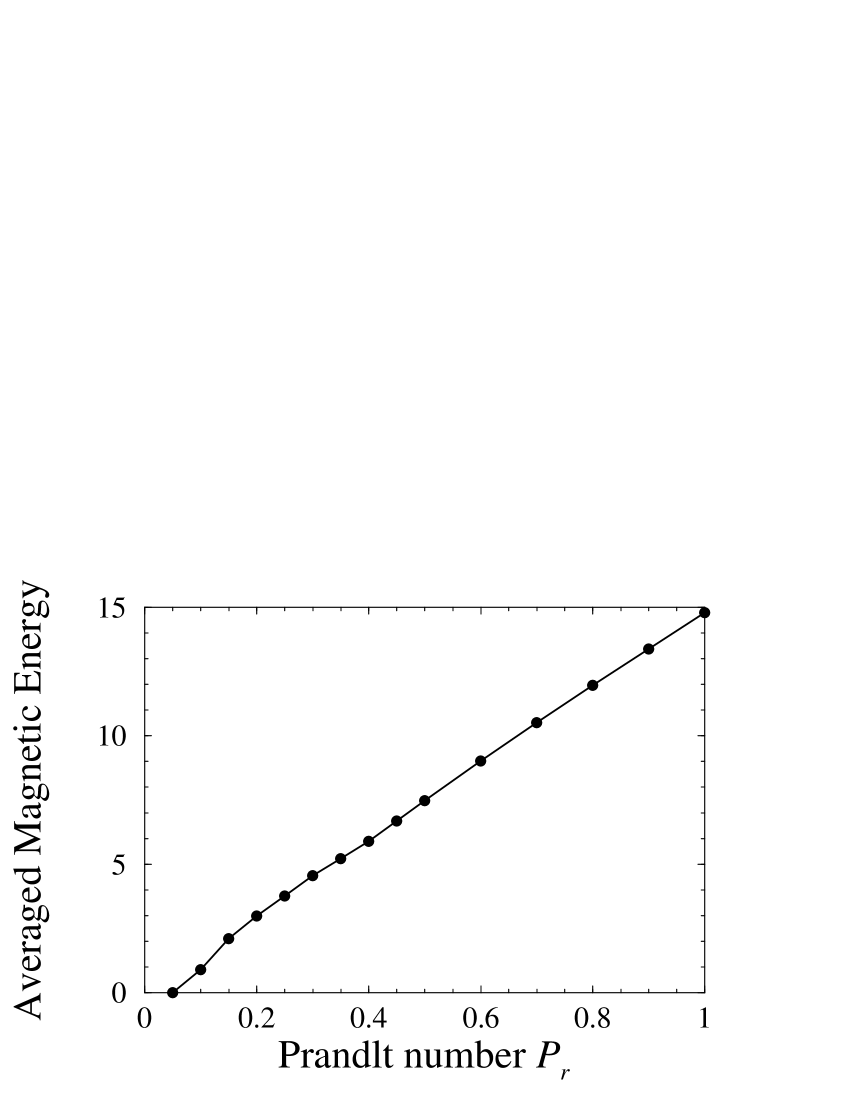
Figure 21: The average magnetic energy $E_{M}$ as a function of $P_{r}$. The parameter values are $R_{\omega}=44000$, $R_{\alpha}=-15.0$ and $Pr=0.5$.

Figure 22: The maximum of $\delta\Omega(r=0.95R_{\odot},\theta)$ as a function of $P_{r}$ when $R_{\omega}=44000$, $R_{\alpha}=-15.0$.

Figure 23: Comparison of the average magnetic energy $E_{M}$ for models with $\alpha$–quenching and smaller $P_{r}$. In this figure, ${R_{\omega}}=44000$, the continuous curve corresponds to the model with $\alpha_{r}=f(r),\eta(r,\theta)=\eta(r),P_{r}=1.0$, the dot–dashed line is for the model with $\alpha$–quenching and the dashed curve for the model with $P_{r}=0.5$ and no $\alpha$-quenching.

Figure 24: Comparison of the maximum of $\delta\Omega(r=0.95R_{\odot},\theta)$ for models with $\alpha$–quenching and smaller values of $P_{r}$. In this figure, ${R_{\omega}}=44000$, the continuous curve corresponds the model with $\alpha_{r}=f(r),\eta(r,\theta)=\eta(r)$, $P_{r}=1.0$, the dot–dashed line represents the model with $\alpha$–quenching and the dashed curve the model with $P_{r}=0.5$.

4.6 Variations in fragmentation level and phase

Finally, in this section we briefly summarise our detailed results concerning the variations in the spatiotemporal fragmentation level (i.e. the maximum radius at which more than one period exists) as well as changes in the phase $\phi$, as a function of the control parameters $R_{\alpha}$ and $P_{r}$ for models with different $\alpha$ and $\eta$ profiles as well as those with nonlinear $\alpha$–quenching.

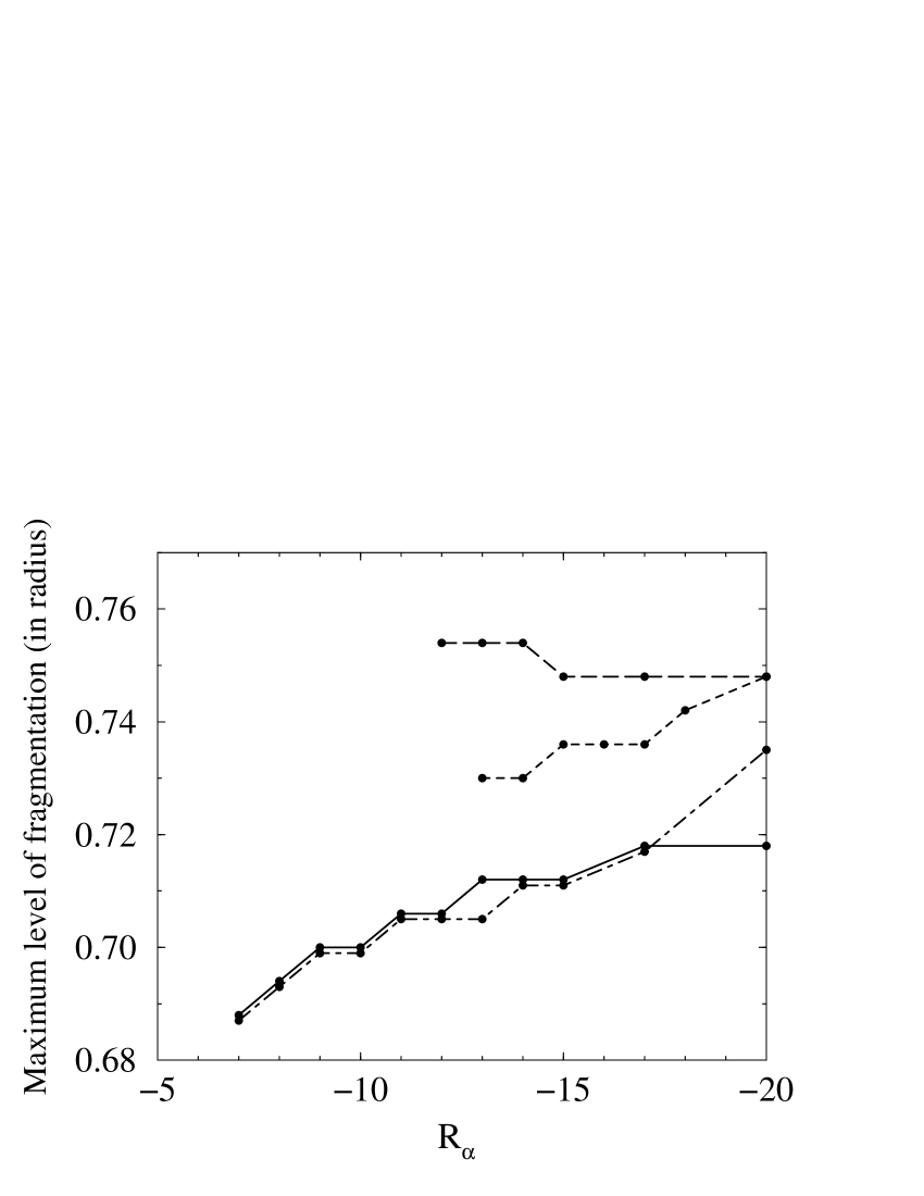
Figure 25: Variation of spatiotemporal fragmentation level for different $\alpha$ and $\eta$ profiles. Here $\Omega(r,\theta)$ is given by the MDI data, $P_{r}=1.0$, $R_{\omega}=44000$ and the continuous curve gives the results for the model with $\alpha_{r}=f(r),\eta(r,\theta)=\eta(r)$, the long-dashed curve the model with $\alpha_{r}=\eta(r,\theta)=1$, the short-dashed curve the model with $\eta(r,\theta)=1$ and the dotted-dashed curve the model with $\alpha_{r}=1$ (slightly displaced downwards for clarity).

Figure 26: Variation of fragmentation level as a function of $R_{\alpha}$, in the presence of $\alpha$–quenching as $P_{r}$ is reduced. Here ${R_{\omega}}=44000$ and the continuous curve gives the results for the model with $\alpha_{r}=f(r),\eta(r,\theta)=\eta(r),P_{r}=1.0$ (slightly displaced upwards for clarity), the dot–dashed line represents the model with $\alpha$–quenching and the dashed curve the model with $P_{r}=0.5$.

Fig. 25 shows the radius of the upper boundary of the region of spatiotemporal fragmentation as a function of $R_{\alpha}$ for different $\alpha$ and $\eta$ profiles at $P_{r}=1$. As can be seen, for intermediate values of $|R_{\alpha}|$, the models with uniform $\eta$ have a higher fragmentation level. Also they also have fragmentation at values of $|R_{\alpha}|$ significantly larger than for the model with a radial dependence of $\eta$. The higher upper boundary of the fragmentation region for such models is associated with the position of the fragmented cells, which are now detached from the bottom boundary, unlike the basic models described earlier (cf. Figs. 7, 17 and 18). At small values of $|R_{\alpha}|$ the removal of the radial dependence on the $\alpha$ profile does not change the maximum height at which fragmentation occurs, and even at higher $|R_{\alpha}|$ it does so only slightly.

We have also studied the position of the boundary of the fragmentation region in models with $\alpha$–quenching as well as lower values of $P_{r}$ and the results are shown in Fig. 26. It can clearly be seen that the quenching of $\alpha$ changes significantly the position and amplitude of the fragmentation. Not only does it start at higher $|R_{\alpha}|$ but it also extends closer to the bottom boundary. The dependence on the Prandtl number is somehow less pronounced. Fragmentation again sets in starts at higher values of $|R_{\alpha}|$ but the position of the fragmentation region is almost the same as that of the basic model with $P_{r}=1$.

Figure 27: Variation of the phase shift $\phi$ as a function of $R_{\alpha}$ for different $\alpha$ and $\eta$ profiles. Here $\Omega(r,\theta)$ is given by the MDI data, $P_{r}=1.0$, $R_{\omega}=44000$ and the continuous curve gives the results for the model with $\alpha_{r}=f(r),\eta(r,\theta)=\eta(r)$, the short-dashed curve the model with $\eta(r,\theta)=1$ and the dotted-dashed curve the model with $\alpha_{r}=1$. We were unable to calculate uniquely the phase shift for the case without radial dependence in both the $\alpha$ and $\eta$ profiles and so we have omitted it.

Further, we studied the shift in phase, $\phi$, between the oscillations near the top and bottom of the dynamo region. Fig. 27 shows the phase shift $\phi$ as a function of $R_{\alpha}$, for different $\alpha$ and $\eta$ profiles. As can be seen, the phase shift can be negative or positive. For the models with $\alpha_{r}=1$, $\phi$ can be either positive or negative, while for the other models it is always positive. We note that the phases shifts for small enough $|R_{\alpha}|$ are correspondingly small, that is the torsional oscillations are all in phase throughout the convection zone.

In Fig. 28 we have plotted the phase shifts for the $\alpha$–quenched models. This shows that $\alpha$–quenching does not dramatically change the behaviour (and the sign) of the phase shifts (apart from reducing it somewhat), for nearly all values of $R_{\alpha}$.

Figure 28: Variation of phase shift $\phi$ as a function of $R_{\alpha}$ in the presence of $\alpha$–quenching. Here ${R_{\omega}}=44000$, the solid line gives the results for the model with $\alpha$ quenching and the dashed line those for the model with $\alpha$–quenching with $g=10^{-2}$.

5 Discussion

We begin by acknowledging the considerable uncertainties and simplifications which are associated with all solar dynamo models, including our own. In particular, in the present context our assumption of uniform density may be important.

We have made a detailed study of a recent proposal in which the recent results of helioseismic observations regarding the dynamical modes of behaviour in the solar convection zone are accounted for in terms of spatiotemporal fragmentation. Originally, support for this scenario came from the study of a particular two dimensional axisymmetric mean field dynamo model operating in a spherical shell, with a semi–open outer boundary condition, which inevitably involved a number of simplifying and somewhat arbitrary assumptions. To demonstrate, to a limited extent at least, the independence of our proposed mechanism from the details of our model, we have shown that this scenario is robust with respect to a number of of plausible changes to the main ingredients of the model, including the $\alpha$ and $\eta$ profiles as well as the inclusion of nonlinear quenching and changes in the Prandtl number. We have also shown the persistence of spatiotemporal fragmentation with respect to the zero order angular velocity (by considering both the MDI and the GONG data sets), as well as under changes in the form of the factor $f(\theta)$ that prescribes the latitudinal dependence of $\alpha$ (by considering $f(\theta)=\sin^{4}\theta\cos\theta$). We further found our model to be capable of producing butterfly diagrams which are in qualitative agreement with the observations. In this way we have found evidence that spatiotemporal fragmentation is not confined to our original model only and that it can occur in more general dynamo models.

Concerning our model, we should note that all our calculations were done with semi–open outer boundary conditions on the toroidal magnetic field (i.e. $\partial B/\partial r=0$). In spite of relatively extensive searches, we have so far been unable to find spatiotemporal fragmentation with pure vacuum boundary conditions ($B=0$). It is interesting to note in this connection that some examples of spatiotemporal bifurcations in the literature (albeit in coupled maps) also have open boundary conditions (see e.g. Willeboordse & Kaneko 1994, Frankel et al. 1994). This may therefore be taken as some tentative support for the idea that spatiotemporal fragmentation may require some sort of open boundary conditions, or that at least it is easier to occur in such settings.

We also made an extensive study of the spatial magnetic field structure as well as the nature of dynamical variations in the differential rotation, including amplitudes and phases, as a function of depth and latitude. Our results demonstrate the presence of three main qualitative spatiotemporal regimes: (i) regimes where there is no deformation of the torsional oscillations bands in the ($r,t$) plane, and hence no changes in phase or period through the convection zone; (ii) regimes where there is spatiotemporal deformation in the oscillatory bands in the ($r,t$) plane, resulting in changes in the phase of the oscillations, but no changes in their period, and (iii) regimes with spatiotemporal fragmentation, resulting in changes both in phase as well as period/behaviour of oscillations, including regimes that are markedly different from those observed at the top, having either significantly reduced periods or non-periodic modes of behaviour. In all three cases, we found that torsional oscillations, resembling those found near marginal excitation, persisted above the fragmentation level.

These modes of behaviour can in principle explain a number of features that have been observed recently. These include:

(a)

Deformations of the type (ii) with or without fragmentation of type (iii), can account for the reversal of the phase of the oscillatory behaviour above and below the tachocline, as reported by Howe et al. (2000a).

(b)

Spatiotemporal fragmentation can explain latitudinal dependence, as fragmentation occurs in both radius/time as well as in latitude/time plots. In particular, it can explain the possibility of oppositely signed tachocline shear at low and high latitudes, as has been found in observations by Howe et al. (2000a). To demonstrate this, we have plotted in Figs. 29 and 30 , the residuals of the differential rotation rate with respect to the radius and the latitude.

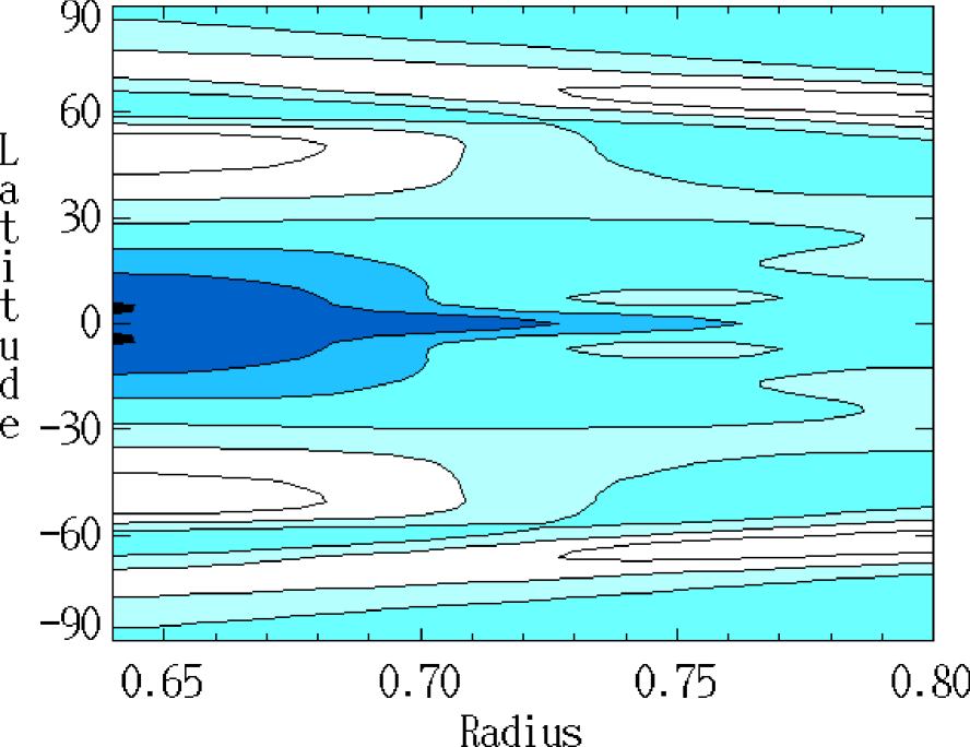
Figure 29: Variation of the perturbation to the zero order rotation rate in latitude and time, revealing the migrating banded zonal flows, after the transients have died out, using the MDI data. Observe that residuals with different signs can occur over small latitude or radii bands. Parameter values are as in Fig. 3.

Figure 30: Variation of the perturbation to the zero order rotation rate in latitude and time, revealing the migrating banded zonal flows, after the transients have died out. Parameter values are as in Fig. 3.

(c)

We observe the penetration of coherent torsional oscillations into all the regions above the fragmentation level, with the penetration extending to slightly greater depths in the case of the GONG data.

(d)

Spatiotemporal fragmentation/bifurcation can in principle explain, purely dynamically, the relationship between the $11$ year and possible $1.3$ year oscillations near the top and bottom of the convection zone. In this connection, note that $11=2^{3}\times 1.3$ years (compatible with the result of Howe et al. 2000a being connected with three period halvings)! It can also explain non-periodic dynamical behaviour (compatible with the findings of Antia & Basu 2000).

Finally, apart from providing a possible theoretical framework for understanding such phenomena, this scenario could, by demonstrating the different qualitative dynamical regimes that can occur in the dynamo models, also be of help in devising strategies for future observations.

- (1) Antia H. M., Basu S., 2000, ApJ, 541, 442
- (2) Brandenburg A., Tuominen I., 1988, Symposium on Solar and Middle Atmosphere Variability, Advances in Space Research, vol. 8, no. 7, 185
- (3) Covas E., Tavakol R., Moss D., Tworkowski A., 2000a, A&A 360, L21
- (4) Covas E., Tavakol R., Moss D., 2000b, A&A 363, L13, also available at http://www.eurico.web.com
- (5) Durney B. R. 2000, Sol. Phys., 196, 1
- (6) Frankel M. L., Roytburd V., Sivashinsky G., 1994, SIAM J. Appl. Math., 54, 1101
- (7) Howard R., LaBonte B. J., 1980, ApJ, 239, L33
- (8) Howe R., et al., 2000a, ApJ Lett., 533, L163
- (9) Howe R., et al., 2000b, Science 287, 2456
- (10) Jennings R. L., 1993, Sol. Phys., 143, 1
- (11) Kichatinov, L. L. 1988, Astronomische Nachrichten, 309, 197
- (12) Kitchatinov, L. L., Rüdiger, G., Küker, M., A&A, 292, 125
- (13) Kitchatinov L. L., Pipin V. V., 1998 Astronomy Reports, 42, 808
- (14) Kitchatinov L. L., Pipin V. V., Makarov V. I., and Tlatov A.G., 1999, Sol. Phys., 189, 227
- (15) Kitchatinov L. L., Mazur M. V., Jardine M., 2000, A&A 359,531
- (16) Küker M., Rüdiger G., Pipin V. V., 1996, A&A, 312, 615
- (17) Kosovichev A. G., Schou J. 1997, ApJ, 482, L207
- (18) Moss D., Brooke J., 2000, MNRAS, 315, 521
- (19) Rüdiger R., Kitchatinov L. L., 1990, A&A 236, 503
- (20) Rüdiger R., Brandenburg A., 1995, A&A 296, 557
- (21) Schuessler, M., 1981, A&A, 94, L17
- (22) Schou J., Antia H. M., Basu S. et al., 1998, ApJ, 505, 390
- (23) Snodgrass H. B., Howard R. F., Webster L., 1985, Sol. Phys., 95, 221
- (24) Willeboordse F. H., Kaneko K., 1994, Phys. Rev. E., 73, 533
- (25) Yoshimura H., 1981, ApJ, 247, 1102