Abstract

We review the main neutrino emission mechanisms in neutron star crusts and cores. Among them are the well-known reactions such as the electron-positron annihilation, plasmon decay, neutrino bremsstrahlung of electrons colliding with atomic nuclei in the crust, as well as the Urca processes and neutrino bremsstrahlung in nucleon-nucleon collisions in the core. We emphasize recent theoretical achievements, for instance, band structure effects in neutrino emission due to scattering of electrons in Coulomb crystals of atomic nuclei. We consider the standard composition of matter (neutrons, protons, electrons, muons, hyperons) in the core, and also the case of exotic constituents such as the pion or kaon condensates and quark matter. We discuss the reduction of the neutrino emissivities by nucleon superfluidity, as well as the specific neutrino emission produced by Cooper pairing of the superfluid particles. We also analyze the effects of strong magnetic fields on some reactions, such as the direct Urca process and the neutrino synchrotron emission of electrons. The results are presented in the form convenient for practical use. We illustrate the effects of various neutrino reactions on the cooling of neutron stars. In particular, the neutrino emission in the crust is critical in setting the initial thermal relaxation between the core and the crust. Finally, we discuss the prospects of exploring the properties of supernuclear matter by confronting cooling simulations with observations of the thermal radiation from isolated neutron stars.

1 Overview

1.1 Introduction

Neutron stars are the most fascinating stars known in the Universe. Indeed, measured masses of these tiny stars are around $M\simeq 1.4\,M_{\odot}$, but they are expected to have very small radii, $R\simeq 10$ km. Accordingly, they possess an enormous gravitational energy, $GM^{2}/R\sim 5\times 10^{53}$ erg $\sim 0.2\,Mc^{2}$, and surface gravity, $GM/R^{2}\sim 2\times 10^{14}$ cm s^-2. Since the gravitational energy constitutes a large fraction of the rest-mass energy, neutron stars are relativistic objects; space-time is essentially curved within and around them, implying they can behave as strong gravitational lenses (e.g., Zavlin et al. 1995). Neutron stars are very dense. Their mean density $\bar{\rho}\simeq 3M/(4\pi R^{3})\simeq 7\times 10^{14}$ g cm^-3 is several times the standard nuclear density, $\rho_{0}=2.8\times 10^{14}$ g cm^-3. The central density is larger, reaching up to (10–20) $\rho_{0}$. Thus, the cores of neutron stars are composed of a strongly compressed nuclear matter. This compression, which cannot be reproduced in laboratory, is provided by the very strong gravitational force. Accordingly, neutron stars can be treated as unique astrophysical laboratories of superdense matter. The main constituents of neutron star cores are thought to be strongly degenerate neutrons with the admixture of protons and electrons, although other particles may also be available.

Observationally, neutron stars manifest themselves in different ways, for instance, as radio pulsars, X-ray pulsars, anomalous X-ray pulsars (e.g., Mereghetti et al. 1998), X-ray bursters (e.g., Lewin et al. 1995), X-ray transients (e.g., Campana et al. 1998), sources of quasiperiodic X-ray oscillations (e.g., Psaltis et al. 1998, Kluzniak 1998), and soft-gamma repeaters (e.g., Cline et al. 1999 and references therein). They are the sources of electromagnetic radiation in all wavelength bands, from radio to hardest gamma-rays, and they are known to work as efficient accelerators of highly energetic particles. Their birth in supernova explosions is accompanied by the most powerful neutrino outburst. One of them was detected by the underground neutrino detectors as a signal of the 1987A supernova explosion in the Large Magellanic Cloud (e.g., Imshennik and Nadezhin 1988, Burrows 1990). Evolution of orbital parameters of the double neutron star binary containing PSR 1913+16, the Hulse–Taylor pulsar, indicates that the binary system emits gravitational waves. Merging neutron stars are thought to be among the best candidates for direct detection of gravitational waves.

In other words, neutron stars are extremely interesting to observe and study theoretically. Their main “mystery” is the equation of state of dense matter in their cores. It cannot be derived from first principles since the exact calculation would require the exact theory of nuclear interactions and the exact many-body theory to account for in-medium effects. While lacking both of these theories, many model equations of state have been constructed in the last decades (e.g., Shapiro and Teukolsky 1983, Glendenning 1996, Weber 1999, Lattimer and Prakash 2000). They vary widely from the soft to the moderate and stiff ones and produce very different structure of neutron stars. This opens a possibility to constrain the equation of state by comparing theory with observations in many ways. The majority of methods are based on the determination (constraint) of the stellar mass and/or radius and the comparison with the mass-radius diagrams for different equations of state. In particular, one can use the data obtained from the mass measurements in close binaries containing neutron stars, the minimum spin periods of the millisecond pulsars, the identification of the kilohertz quasi-periodic oscillations with the orbital frequency in the last stable orbit, and from other related methods. Unfortunately, no decisive argument has been given so far in favor of the stiff, moderate or soft equations of state. One can definitely rule out only the ultra-soft equations of state which give the maximum stellar mass lower than $1.44\,M_{\odot}$, the accurately measured mass of the Hulse–Taylor pulsar (Thorsett and Chakrabarty 1999).

In this review we focus on another method to explore the internal structure of neutron stars — by comparing the theory of neutron star cooling with observations of the thermal radiation from the surfaces of isolated neutron stars. For about $10^{5}$–$10^{6}$ years after their birth in supernova explosions, neutron stars cool mainly via neutrino emission from their interiors. Although their matter is very dense, they become fully transparent for neutrinos about 20 seconds after the birth (e.g., Burrows and Lattimer 1986, Prakash et al. 1997). Thus, the neutrinos produced in numerous reactions leave neutron stars freely, providing a powerful source of cooling. Therefore, it is important to study the whole variety of neutrino reactions in different neutron star layers in order to analyze the cooling. Some mechanisms have been reviewed not long ago by Bisnovatyi-Kogan (1989), Pethick (1992), Itoh et al. (1996), and Yakovlev et al. (1999b). More references to the original and review papers are given in subsequent chapters.

The present review differs from other papers in several respects. First, we discuss the neutrino mechanisms in all neutron star layers, from the crust to the inner core, paying attention to open theoretical problems. Second, we consider the neutrino emission in the non-superfluid and non-magnetized matter as well as in the presence of superfluidity of baryons and the possible strong magnetic field. In particular, we analyze the neutrino emission due to Cooper pairing of baryons, which is forbidden in non-superfluid matter, and the synchrotron neutrino emission of electrons forbidden without the magnetic field. Third, we present the results in a unified form, convenient for use in neutron star cooling codes. Fourth, we discuss the relative importance of all these neutrino reactions for the various stages of the cooling.

The review is organized as follows. In the next section, we describe briefly the structure of neutron stars. In Chapt. 2 we analyze various neutrino reactions in neutron star crusts. In Chapt. 3 we describe neutrino processes in non-superfluid and non-magnetized neutron star cores. In Chapt. 4 we consider the reactions in superfluid and magnetized cores. Finally, in Chapt. 5 we discuss the efficiency of various reactions for neutron star cooling, present new results of cooling simulations and compare them with observations.

1.2 Structure of neutron stars

A neutron star can be subdivided into the atmosphere and four internal regions: the outer crust, the inner crust, the outer core, and the inner core.

The atmosphere is a thin layer of plasma which determines the spectrum of thermal electromagnetic radiation of the star. In principle, this radiation contains valuable information on the stellar parameters (temperature, gravitational acceleration and chemical composition of the surface, magnetic field, etc.) and, as a result, on the internal structure. Geometrical depth of the atmosphere varies from some ten centimeters in a hot star down to some millimeters in a cold one.

Neutron star atmospheres have been studied theoretically by many authors (see, e.g., review papers by Pavlov et al. 1995, Pavlov and Zavlin 1998, and references therein). Construction of the atmosphere models, especially for cold stars with the effective surface temperature $T_{s}\;\raise 1.29167pt\hbox{$<$\kern-7.5pt\raise-4.73611pt\hbox{$\sim$}}\;10^{6}$ K and strong magnetic fields 10¹¹–10¹⁴ G, is incomplete owing to serious theoretical problems concerned with the calculation of the equation of state and spectral opacity of the atmospheric plasma.

The outer crust (outer envelope) extends from the bottom of the atmosphere to the layer of density $\rho_{\rm d}\approx 4\times 10^{11}$ g cm^-3 and has a depth of a few hundred meters (Shapiro and Teukolsky 1983). It is composed of ions and electrons. A very thin (no more than several meters in a hot star) surface layer contains non-degenerate electron gas but in the deeper layers the electrons are degenerate. At $\rho\;\raise 1.29167pt\hbox{$<$\kern-7.5pt\raise-4.73611pt\hbox{$\sim$}}\;10^{4}$ g cm^-3 the electron plasma may be non-ideal and the ionization may be incomplete. At higher densities the electron gas is almost ideal and the atoms are fully ionized, being actually bare atomic nuclei. As the electron Fermi energy grows with $\rho$, the nuclei capture electrons and become neutron-rich (Sect. 2.7). At the base of the outer crust ($\rho=\rho_{\rm d}$) the neutrons start to drip from the nuclei and form a free neutron gas.

The state of the degenerate electrons is characterized by the Fermi momentum $p_{{\rm F}e}$ or the relativistic parameter $x_{r}$:

$$p_{{\rm F}e}=\hbar(3\pi^{2}n_{e})^{1/3},\quad x_{r}={p_{{\rm F}e}\over m_{e}c}\approx 100.9\left({\rho_{12}Y_{e}}\right)^{1/3},$$ (1)

where $Y_{e}=n_{e}/n_{b}$ is the number of electrons per baryon, $n_{e}$ is the number density of electrons, $n_{b}$ the number density of baryons, and $\rho_{12}$ is the mass density in units of $10^{12}$ g cm^-3. The electron degeneracy temperature is

$$T_{\rm F}=(\sqrt{1+x_{r}^{2}}-1)\,T_{0},\quad T_{0}\equiv{m_{e}c^{2}\over k_{\rm B}}\approx 5.930\times 10^{9}~{}~{}{\rm K},$$ (2)

where $k_{\rm B}$ is the Boltzmann constant. The chemical potential of strongly degenerate electrons equals $\mu_{e}=m_{e}\,(1+x_{r}^{2})^{1/2}$. The electrons become relativistic at $x_{r}\gg 1$, i.e., at $\rho\gg 10^{6}$ g cm³.

The state of the ions (nuclei) in a one-component ion plasma is determined by the ion-coupling parameter

$$\Gamma={Z^{2}e^{2}\over ak_{\rm B}T}\,\approx\,0.225\,x_{r}\,{Z^{5/3}\over T_{8}},$$ (3)

where $Ze$ is the nuclear charge, $a=[3/(4\pi n_{i})]^{1/3}$ is ion–sphere (Wigner–Seitz cell) radius, $n_{i}$ is the number density of ions, and $T_{8}$ is the temperature in units of $10^{8}$ K. For the densities and temperatures of interest for neutrino reactions (Chapt. 2) the ions constitute either a strongly coupled Coulomb liquid ($1<\Gamma<\Gamma_{m}$), or a Coulomb crystal ($\Gamma>\Gamma_{m}$), where $\Gamma_{m}\approx 172$ corresponds to the solidification of a classical one-component Coulomb liquid into the body centered cubic (bcc) lattice (Nagara et al. 1987). The corresponding melting temperature is

$$T_{m}={Z^{2}e^{2}\over ak_{\rm B}\Gamma_{m}}\approx 1.32\times 10^{7}Z^{5/3}\left({\rho_{12}Y_{e}}\right)^{1/3}~{}~{}{\rm K}.$$ (4)

An important parameter of a strongly coupled ion system is the ion plasma temperature

$$T_{p}={\hbar\omega_{p}\over k_{\rm B}}\approx 7.83\times 10^{9}\left({ZY_{e}\rho_{12}\over A_{i}}\right)^{1/2}~{}{\rm K},$$ (5)

determined by the ion plasma frequency $\omega_{p}=\left({4\pi Z^{2}e^{2}n_{i}/m_{i}}\right)^{1/2}$, where $m_{i}\approx A_{i}m_{u}$ is the ion mass and $m_{u}=1.66055\times 10^{-24}$ g is the atomic mass unit. The plasma temperature characterizes thermal vibrations of the ions. If $T\;\raise 1.29167pt\hbox{$>$\kern-7.5pt\raise-4.73611pt\hbox{$\sim$}}\;T_{p}/8$, the vibrations can be treated classically, while at $T\ll T_{p}$ they are essentially quantum. In the layers of interest for neutrino reactions, the transition from the classical to the quantum-mechanical regime takes place at temperatures lower than $T_{m}$.

Vibrational properties of the bcc Coulomb crystal of ions immersed in the uniform electron gas are well known (e.g., Pollock and Hansen 1973). The spectrum contains three phonon branches. Generally, the phonon frequencies are $\omega_{s}(k)\sim\omega_{p}$ ($s=$ 1, 2, 3). At large wavelengths, $k\to 0$, two branches behave as transverse acoustic modes ($\omega_{s}\propto k$ for $s=1$ or 2), while the third is longitudinal and optical ($\omega_{s}\to\omega_{p}$). However, because of the compressibility of the electron gas, the optical mode turns into the acoustic one at very small $k$.

The inner crust (inner envelope) extends from the density $\rho_{\rm d}$ at the upper boundary to $\sim 0.5\rho_{0}$ at the base. Its thickness can be as large as several kilometers. The inner crust is composed of the electrons, free neutrons and neutron-rich atomic nuclei (Negele and Vautherin 1973, Pethick and Ravenhall 1995). The fraction of free neutrons increases with density. At the bottom of the crust, in the density range from $10^{14}$ to $1.5\times 10^{14}$ g cm^-3, the nuclei can be non-spherical and form clusters (Lorenz et al. 1993; Pethick and Ravenhall 1995). The nuclei disappear completely at the crust-core interface.

The free neutrons $n$ in the inner crust may be superfluid. The superfluidity is thought to be produced by Cooper pairing via the attractive part of the singlet-state neutron-neutron interaction. Superfluidity occurs when temperature falls below the critical temperature $T_{cn}$. References to the numerous microscopic calculations of $T_{cn}$ can be found, for instance, in Yakovlev et al. (1999b). The results are very sensitive to the model of $nn$-interaction and the many-body theory employed. The most important common feature is that $T_{cn}$ increases with density at $\rho\;\raise 1.29167pt\hbox{$>$\kern-7.5pt\raise-4.73611pt\hbox{$\sim$}}\;\rho_{\rm d}$, reaches maximum (from $10^{8}$ to $10^{11}$ K, depending on the microscopic model) at subnuclear densities, and decreases to zero at $\rho\sim\rho_{0}$. The initial increase is associated with the growth of the effective $nn$ interaction strength with increasing density. The decrease of $T_{cn}$ occurs where the effective singlet-state $nn$ attraction turns into repulsion. In the models which take into account in-medium (polarization) effects $T_{cn}$ is typically several times lower than in the models which ignore these effects. The critical temperature is sensitive to the values of the effective neutron mass which determines the density of states of neutrons near the Fermi surface: the lower the effective mass the smaller $T_{cn}$. Note, that the bound nucleons within atomic nuclei can also be in superfluid state.

The outer core occupies the density range $0.5\rho_{0}\;\raise 1.29167pt\hbox{$<$\kern-7.5pt\raise-4.73611pt\hbox{$\sim$}}\;\rho\;\raise 1.29167pt\hbox{$<$\kern-7.5pt\raise-4.73611pt\hbox{$\sim$}}\;2\rho_{0}$ and can be several kilometers deep. It is composed mainly of neutrons with some admixture (several percent by number) of protons $p$ and electrons $e$ (the so called standard nuclear composition). For $\rho\;\raise 1.29167pt\hbox{$>$\kern-7.5pt\raise-4.73611pt\hbox{$\sim$}}\;\rho_{0}$, where the electron chemical potential $\mu_{e}>m_{\mu}c^{2}=105.7$ MeV, a small fraction of muons ($\mu$) appear. The composition of $npe$-matter at densities below the muon threshold is determined by the conditions of electric neutrality and beta-equilibrium with respect to the reactions $n\to p+e+\bar{\nu}_{e}$, $\;p+e\to n+\nu_{e}$, where $\nu_{e}$ and $\bar{\nu}_{e}$ stand for electron neutrino and antineutrino, respectively. The electric neutrality requires the electron and proton number densities be equal, $n_{p}=n_{e}$. Beta equilibrium implies then the following relationship between chemical potentials of the particles: $\mu_{n}=\mu_{p}+\mu_{e}$. The neutrino chemical potential is ignored here since neutron stars are transparent for neutrinos. In the presence of muons the condition of electric neutrality reads $n_{p}=n_{e}+n_{\mu}$, and the equilibrium with respect to the weak processes involving muons implies $\mu_{e}=\mu_{\mu}$, in addition to the beta-equilibrium condition $\mu_{n}=\mu_{p}+\mu_{e}$. All $npe\mu$-plasma components are strongly degenerate. The electrons and muons form almost ideal Fermi-gases. The electrons are ultrarelativistic, while the muons are nonrelativistic near the threshold of their appearance and become moderately relativistic at higher densities. The neutrons and protons, which interact via nuclear forces, constitute a strongly non-ideal, non-relativistic Fermi-liquid.

With increasing density, the particle Fermi energies grow, so that new particles can be created. The appearance of new particles in the inner core is discussed below.

Let us emphasize that a self-consistent quantum theory of matter of supernuclear density has not been constructed yet. Many theoretical equations of state have been proposed (e.g., Lattimer and Prakash 2000) which can be divided conventionally into the soft, moderate and stiff with respect to the compressibility of matter. These equations of state vary considerably from one another.

Almost all microscopic theories predict the appearance of neutron and proton superfluids in neutron star cores (see Yakovlev et al. 1999b for references). These superfluids are believed to be produced by the $nn$ and $pp$ Cooper pairing due to the attractive part of the nuclear potential and can be characterized by the critical temperatures $T_{cn}$ and $T_{cp}$. The proton superfluidity is accompanied by superconductivity (most likely, of second type) and affects the evolution of the internal magnetic field (see, e.g., Ruderman 1991).

Owing to a sufficiently low concentration of protons, the proton pairing is produced by the singlet-state attractive part of the $pp$ interaction. Although the singlet-state $nn$ interaction in neutron star cores is repulsive, as discussed above, some part of the triplet-state $nn$ interaction is attractive leading to neutron pairing. As in the crust, the microscopic theories give very model-dependent values of $T_{cn}$ and $T_{cp}$. According to these theories, the density dependence of $T_{cn}$ has a maximum at supranuclear density. The maximum values vary from $10^{8}$ K to about $10^{10}$ K in different models. Usually, the dependence $T_{cp}(\rho)$ also has a maximum at some supernuclear density. The maximum values fall in the same range as $T_{cn}$.

The critical temperatures $T_{cn}$ and $T_{cp}$ are much more sensitive to the microscopic models of dense matter than the pressure, the main ingredient of the equation of state. There is no direct link between these quantities: the pressure is the bulk property determined by the entire Fermi-seas of the particles, while the superfluidity is the phenomenon occurring near the Fermi surfaces. However, both the superfluidity and pressure depend on the repulsive core of the nucleon-nucleon interaction. For a less repulsive (more attractive) core, one has a softer equation of state and higher $T_{c}$. Therefore, the superfluid state of neutron star cores is related in some way to the equation of state. As in the crust, $T_{c}$ in the stellar core is sensitive to in-medium effects.

The outer core of a low-mass neutron star extends all the way to the center. More massive stars possess also the inner core. It can be several kilometers in radius and have a central density as high as $(10-15)\rho_{0}$. The composition and equation of state of the inner core are poorly known. Several hypotheses have been discussed in the literature and it is impossible to reject any of them at present:

(1) Large proton fraction ($>11\%$) and/or hyperonization of matter — the appearance of $\Sigma$, $\Lambda$ and other hyperons (see, e.g., Shapiro and Teukolsky 1983, Balberg and Barnea 1998, Balberg et al. 1999). The fractions of $p$ and $e$ may become so high that the powerful $npe$ direct Urca process of neutrino emission becomes allowed (Lattimer et al. 1991) as well as the similar reactions involving hyperons (Prakash et al. 1992). In these cases the neutrino luminosity of the star is enhanced by 5–6 orders of magnitude (Sect. 3.3) compared to the standard neutrino luminosity produced mainly by the modified Urca processes (Sect. 3.4). This accelerates considerably the cooling of neutron stars.

(2) The second hypothesis, proposed in different forms by Bahcall and Wolf (1965a, b), Migdal (1971), Sawyer (1972), and Scalapino (1972), assumes the appearance of pion condensation. The condensates soften the equation of state and enhance the neutrino luminosity by allowing the reactions of the direct Urca type (Sect. 3.8). However, many modern microscopic theories of dense matter predict weakly polarized pionic degrees of freedom which are not in favor of pion condensation (Pethick, 1992).

(3) The third hypothesis predicts a phase transition to the strange quark matter composed of almost free $u$, $d$ and $s$ quarks with small admixture of electrons (see Weber 1999 for review). In these cases the neutrino luminosity is thought to be considerably higher than the standard luminosity due to switching on the direct Urca processes involving quarks (Sect. 3.8).

(4) Following Kaplan and Nelson (1986), Nelson and Kaplan (1987) and Brown et al. (1988), several authors considered the hypothesis of kaon condensation. Similarly to pion condensates, kaon condensates may also enhance the neutrino luminosity by several orders of magnitude (Sect. 3.8). A critical analysis of the theories of kaon condensation was given by Pandharipande et al. (1995). The present state of the theories has been reviewed, for instance, by Ramos et al. (2000).

We see that the composition of dense matter affects the neutrino emission and, hence, neutron star cooling. These effects are discussed in the next chapters. Notice that in all cases the matter can be in superfluid state. For instance, Takatsuka and Tamagaki (1993, 1997a, b, c) calculated the neutron and proton superfluid gaps in the matter with pion condensates. The same authors (Takatsuka and Tamagaki 1995) studied nucleon superfluidity in the presence of kaon condensation. The pion or kaon condensates mix strongly the neutron and proton states and may induce the triplet-state pairing of quasi-protons. If hyperons appear in the $npe$-matter, they can also be superfluid (Balberg and Barnea 1998). In all these cases the critical temperatures are of the same order of magnitude as $T_{cn}$ and $T_{cp}$ in ordinary $npe$ matter. Some authors discussed the superfluidity of quark matter (e.g., Bailin and Love 1984, Iwasaki 1995, Schaab et al. 1996, 1997a, Schaäfer and Wilczek 1999, Rajagopal 1999). In this case the situation is more intriguing since the theoretical models predict two possibilities. The first is pairing of like quarks leading to the superfluid gaps of a few MeV and critical temperatures of a few times $10^{10}$ K, not much higher than $T_{c}$ in $npe$ matter. The second is pairing of different quarks ($ud$, $us$, $ds$) which could be much more efficient producing $k_{\rm B}T_{c}$ up to 50 MeV, about one-tenth of the quark Fermi energy ($\sim 500$ MeV). This pairing requires the Fermi momenta of different quarks to be sufficiently close; it weakens with increasing the difference of these Fermi momenta. If realized the pairing leads to the strongest superfluidity and superconductivity of dense matter (often referred to as color superconductivity since Cooper pairs of quarks possess color). Cooling of neutron stars containing quark matter with superfluidity of two types has been analyzed recently in several papers (e.g., Page et al. 2000).

Another complication comes from the possible existence of strong magnetic fields in neutron star interiors. It is widely accepted that the field on the surfaces of radio pulsars can be as large as $10^{13}$ G. Thompson and Duncan (1996) predicted theoretically the existence of the so-called magnetars, neutron stars with the magnetic fields several orders of magnitude stronger than in ordinary radio pulsars. Some of the soft-gamma repeaters or anomalous X-ray pulsars may be magnetars (e.g., Colpi et al. 2000), although this interpretation requires further confirmation (e.g., Harding et al. 1999). It is natural to assume that the internal magnetic field can be even higher than that on the surface. The internal field can be confined in the crust or be distributed over the entire star. If protons or hyperons are superfluid (superconducting) in the core, the magnetic field would likely exist in the form of fluxoids (the quantized magnetic flux tubes, Sect. 4.10). In the absence of superconductivity, the magnetic field is thought to be microscopically uniform. A strong magnetic field can affect the neutrino reactions and stellar cooling. In particular, a quasi-uniform magnetic field opens a new neutrino reaction, the synchrotron neutrino emission by electrons (Sect. 2.4), which is forbidden without the magnetic field. The effects of magnetic fields on the neutrino reactions in the crust and core are studied in Chapts. 2, and 4, respectively. Some of the magnetic field effects on neutron star cooling are analyzed in Chapt. 5.

2 Neutrino emission from neutron star crusts

2.1 Main neutrino reactions

(a) Reactions and their properties

In this chapter we consider various neutrino reactions in neutron star crusts. These reactions are important sources of energy loss in a cooling neutron star at initial stages of the thermal relaxation in the stellar interior (first 10-100 years of the neutron star life, Chapt. 5). In addition, studying neutrino emission from the stellar crusts is an excellent introduction to the problem of neutrino reactions in the stellar cores (Chapts. 3 and 4).

While considering neutron star crusts, we deal with an extremely rich spectrum of physical conditions ranging from an “ordinary” electron-ion plasma in the outermost surface layers to the strongly coupled plasma of atomic nuclei (or their clusters), electrons and free neutrons near the crust-core interface (Sect. 1.2). The problem is complicated further by the possible presence of very strong magnetic fields and nucleon superfluidity (of free neutrons and nucleons within atomic nuclei) in the inner crust. Accordingly, there is a variety of neutrino emission mechanisms that may be important in different crust layers for certain temperature intervals. In order to simplify our consideration, we mainly restrict ourselves only to those mechanisms which may affect the thermal evolution of neutron stars (Chapt. 5). Therefore we will not consider in detail the neutrino emission from the outer layers of density $\rho\;\raise 1.29167pt\hbox{$<$\kern-7.5pt\raise-4.73611pt\hbox{$\sim$}}\;10^{10}$ g cm^-3. These layers contain a negligible fraction of the neutron star mass and cannot be the sources of significant neutrino energy losses. Moreover, we will consider temperatures $T\;\raise 1.29167pt\hbox{$<$\kern-7.5pt\raise-4.73611pt\hbox{$\sim$}}\;10^{10}$ K which are expected in the crusts of cooling neutron stars older than, say, one minute. At such temperatures, neutron stars become fully transparent to neutrinos. In addition, there is no need to study too low temperatures, $T\;\raise 1.29167pt\hbox{$<$\kern-7.5pt\raise-4.73611pt\hbox{$\sim$}}\;3\times 10^{6}$ K, because the neutrino emission becomes too weak to affect the stellar evolution.

Therefore, under the conditions of study, the electrons constitute strongly degenerate, ultrarelativistic, almost ideal electron gas. This greatly simplifies our treatment of the neutrino emission. The atomic nuclei mainly form strongly coupled Coulomb liquid or crystal, and may form a liquid crystal near the crust base. Free neutrons which appear in the inner crust constitute a strongly interacting Fermi liquid. All of these properties of the matter affect the neutrino emission.

Our primary goal is to obtain the neutrino emissivity $Q$ (energy carried away by neutrinos and antineutrinos per second per unit volume) in various reactions. It is the total emissivity which is the most important for the thermal evolution of neutron stars (Chapt. 5). Thus, we will study neither the spectrum, nor the angular distribution of the emitted neutrinos, nor the neutrino scattering and propagation in the plasma (which would be most important for proto-neutron stars, see, e.g., Prakash et el. 1997).

The calculations of the emissivities are based on the Weinberg-Salam-Glashow theory of electroweak interactions (e.g., Okun’ 1984). Typical energies of the emitted neutrinos are of the order of the thermal energy, $k_{\rm B}T$, or higher. For temperatures of practical interest, $T\;\raise 1.29167pt\hbox{$>$\kern-7.5pt\raise-4.73611pt\hbox{$\sim$}}\;3\times 10^{6}$ K, these energies are higher than the possible neutrino masses. Accordingly, one can employ the approximation of massless neutrinos while calculating the neutrino emissivity. In practical expressions we will take into account the generation of neutrinos and antineutrinos of three flavors ($\nu_{e}$, $\nu_{\mu}$, and $\nu_{\tau}$) although the expressions will be presented in the form ready to incorporate any number of neutrino flavors. On the other hand, the thermal energies of interest are much smaller than the intermediate boson mass, $\sim$ 80 GeV. This enables us to use the reduced 4-tail Feynman weak interaction diagrams instead of the more complicated pairs of three-tail diagrams tied by the intermediate-boson exchange line.

The neutrino processes in the crusts of cooling neutron stars have much in common with those in normal stars at the late stages of their evolution (particularly, in presupernovae) or in the cores of white dwarfs. These processes have been studied since the beginning of the 1960s in a number of seminal papers (see, e.g., Pinaev 1963, Fowler and Hoyle 1964, Beaudet et al. 1967, and references therein, as well as references in subsequent sections of this chapter). The early studies were conducted in the framework of an old, simplified Fermi theory of weak interactions and required revision in the 1970s after the Weinberg-Salam-Glashow theory was widely accepted. However, the revision consisted only of simple replacements of the weak interaction normalization constants associated with the inclusion of neutral currents. It did not destroy the earlier results. Thus, we will not put special emphasis on the type of the weak interaction theory, used in the references, assuming the reader will not be confused by the somewhat different normalization constants. The general neutrino processes in stellar interior have been reviewed by several authors, for instance, by Imshennik and Nadyozhin (1982), Bisnovatyi-Kogan (1989), Itoh et al. (1996).

The main neutrino reactions in neutron star crusts are listed in Table 1. The electron-positron pair annihilation, plasmon decay, electron synchrotron neutrino emission, and photoneutrino emission involve electrons (positrons) and collective electromagnetic modes (associated mainly with electrons). The appropriate neutrino emissivities can be calculated precisely as a function of two parameters, the temperature and electron number density. We can precisely determine these emissivities for any given model of dense matter.

The next reaction in Table 1 is the neutrino bremsstrahlung due to scattering of electrons off atomic nuclei. It is the process based solely on weak and electromagnetic interactions but its emissivity depends on the correlations between the nuclei and on the proton charge distribution within the nuclei. Thereby, it is linked to a specific model of dense matter, although it does not vary strongly from one model to another.

Other processes in Table 1 involve weak nucleon reactions. They are subdivided into two groups: the beta decay reactions (including Urca processes) and the processes connected with strong interaction of free neutrons in the inner neutron star crust (neutrino emission in neutron-neutron collisions, in neutron-nucleus collisions, and due to Cooper pairing of free neutrons). The emissivities of these processes depend on a microscopic model of the matter (e.g., on the critical temperature of superfluidity of free neutrons).

Table 1: Main neutrino processes in a neutron star crust^∗)

No.	Process		Sect.
1	$e^{-}e^{+}$ pair annihilation	$ee^{+}\to\nu\bar{\nu}$	2.2
2	plasmon decay	$\gamma\to\nu\bar{\nu}$	2.3
3	electron synchrotron	$e\to e\nu\bar{\nu}$	2.4
4	photoneutrino emission	$e+\gamma\to e\nu\bar{\nu}$	2.5
5	electron-nucleus bremsstrahlung	$e(A,Z)\to e(A,Z)\nu\bar{\nu}$	2.6
6	beta processes (including Urca)	$e(A,Z)\to(A,Z-1)\nu_{e}\quad(A,Z-1)\to(A,Z)e\bar{\nu}_{e}$	2.7
7	Cooper pairing of neutrons	$nn\to\nu\bar{\nu}$	2.8
8	neutron-neutron bremsstrahlung	$nn\to nn\nu\bar{\nu}$	2.8
9	neutron-nucleus bremsstrahlung	$n(A,Z)\to n(A,Z)\nu\bar{\nu}$	2.8

∗) $\gamma$ means a plasmon or photon; $(A,Z)$ stands for an atomic nucleus

(b) Illustrative model: ground-state matter

For illustration purposes, we will mainly use the model of ground-state matter in the neutron star crust. This state of matter is energetically most favorable. Its properties will be described using the results of Haensel and Pichon (1994) at densities below the neutron drip density and the results of Negele and Vautherin (1973) and Oyamatsu (1993) at higher densities. The model assumes that only one nuclear species is present at a given density (or pressure), which leads to discontinuous variations of the nuclear composition with density (pressure). Thermal effects on the composition of dense matter are small and can be ignored.

The model of ground-state matter (discussed in Sect. 2.7 in more details) is based on the properties of atomic nuclei The nuclei can be treated as spherical almost everywhere in the crust although they might be non-spherical in the deepest layer of the inner crust ($10^{14}$ g cm${}^{-3}\leq\rho\leq 1.5\times 10^{14}$ g cm^-3). We describe this layer adopting model I of Oyamatsu (1993). The layer consists of four sublayers. The first sublayer below the crust of spherical nuclei contains the rod-like nuclei. It is followed by a sublayer of the slab-like nuclei, and by the two sublayers with the roles of the nuclear matter and neutron matter reversed, the rod-like one (neutron gas tubes in nuclear matter) and the “Swiss cheese” one (spherical neutron gas bubbles in nuclear matter). The latter is an analog of the phase of spherical nuclei and is the last phase in the neutron-star crust. At higher density the nuclei dissolve into the uniform matter of the neutron star core.

The properties of atomic nuclei in all layers of neutron star crusts are conveniently described by introducing the Wigner–Seitz cells of different geometries (e.g., spheres for the spherical nuclei, or cylinders for the rod-like ones). Following Oyamatsu (1993), we employ the parameterization of the local neutron and proton number density distributions within a Wigner–Seitz cell of the form

$$n_{j}(r)=\left\{\begin{array}[]{ll}(n_{j}^{\rm in}-n_{j}^{\rm out})\left[1-\left(r\over R_{j}\right)^{t_{j}}\right]^{3}+n_{j}^{\rm out},&r<R_{j},\\ n_{j}^{\rm out},&r\geq R_{j},\end{array}\right.$$ (6)

where $r$ is the distance from the cell center (e.g., from the center of the sphere or from the axis of the cylinder), $j=n$ or $p$, and $n_{j}^{\rm in}$, $n_{j}^{\rm out}$, $t_{j}$ and $R_{j}$ are the adjustable parameters. These parameters are presented by Oyamatsu (1993) at several values of the density $\rho$ for the spherical and nonspherical nuclei. For spherical nuclei, they are consistent with those following from the results of Negele and Vautherin (1973).

Kaminker et al. (1999a) interpolated the fit parameters (separately within each phase). The interpolation smears out jumps in the nuclear composition with increasing $\rho$, but they have little effect on the neutrino emission. Notice that $n_{n}^{\rm out}=0$ at $\rho$ below the neutron drip density. In the phases with spheres, rods and slabs, $n_{p}^{\rm out}=0$, and $n_{n}^{\rm out}$ describes the number density of free neutrons, while the region $r<R_{n}$ is occupied by the nucleus itself (with $n_{n}^{\rm in}>n_{n}^{\rm out}$). In the two last “bubble” phases with the roles of nuclear matter and neutron matter reversed, $n_{p}^{\rm out}\neq 0$, and $n_{j}^{\rm out}>n_{j}^{\rm in}$, i.e., the local number density of neutrons and protons increases with distance $r$ from the center of the Wigner–Seitz cell. With increasing $\rho$, the nucleon density profiles become smoother, resembling uniform matter. Thus, Kaminker et al. (1999a) obtained a simple analytic description of the local density profiles of neutrons and protons for the ground-state matter throughout the neutron star crust. This description will be referred to as the smooth composition model of ground-state matter.

(c) Illustrative figures

To make our analysis less abstract, in Figs. 1–4 we display the density dependence of the neutrino emissivity of the main neutrino processes for the four values of the temperature, $T=3\times 10^{9}$, $10^{9}$, $3\times 10^{8}$, and $10^{8}$ K, respectively. We adopt the ground–state model of matter described above and extend the density range to somewhat lower values in order to show clearly the efficiency of different neutrino mechanisms. We exclude densities higher than $3\times 10^{13}$ g cm^-3 (near the bottom of the neutron star crust); they will be considered in Sects. 2.6–2.9.

The neutrino emissivities due to the pair annihilation (‘pairs’, Sect. 2.2) and synchrotron radiation of electrons (‘syn’, Sect. 2.4) are presented for the three values of the magnetic field $B=10^{12}$, $10^{13}$ and $10^{14}$ G in a magnetized neutron-star crust. At the highest temperature, $T=3\times 10^{9}$ K, the pair-annihilation emissivity is actually independent of $B$ as long as $B\;\raise 1.29167pt\hbox{$<$\kern-7.5pt\raise-4.73611pt\hbox{$\sim$}}\;10^{14}$ G. Other curves are calculated neglecting the effect of the magnetic fields (for $B=0$). The curve ‘plasma’ refers to the neutrino plasmon decay process (Sect. 2.3), ‘photo’ corresponds to the photoneutrino reaction (Sect. 2.5). The emissivity of the latter process is taken from Itoh et al. (1989, 1996). Finally, ‘brems’ is the neutrino bremsstrahlung due to the electron-nucleus scattering. Its emissivity is calculated using the formalism described in Sect. 2.6. The jumps of the curves in Figs. 1–4 are mainly associated with the changes of nuclear composition. These changes affect each curve in a different way. Neutrino bremsstrahlung due to the electron-nucleus scattering is affected in the entire density range displayed, since the jumps of the atomic charge number influence directly Coulombic electron-nucleus interaction. The neutrino emissivities of other processes are determined by the electron and positron number densities which are almost continuous at low densities, below the neutron drip density, but have quite pronounced jumps at higher densities. Thus, the appropriate curves are nearly continuous below the neutron drip density. At higher densities, the emissivity of the synchrotron radiation is almost independent of the electron number density and thus remains smooth, while the emissivity of the plasmon decay reflects the jumps of the electron number density (see Sect. 2.3).

We return to Figs. 1–4 while analyzing various neutrino processes in subsequent sections. We adopt the units in which $\hbar=c=k_{\rm B}=1$, but give the final expressions in the standard physical units.

Figure 1: Density dependence of neutrino emissivities from ground-state matter of the neutron-star crust due to various mechanisms at $T=3\times 10^{9}$ K. Curves ‘syn (12)’, ‘(13)’, and ‘(14)’ refer to the synchrotron mechanism (Sect. 2.4) at $B=$ 10¹², 10¹³ and 10¹⁴ G, respectively. Curve ‘pairs’ corresponds to the neutrino emission due to the annihilation of electron-positron pairs; it is almost independent of $B$ at given $T$. Other curves are for $B=0$: ‘brems’ — electron–nucleus bremsstrahlung (Sect. 2.6); ‘plasma’ — plasmon decay (Sect. 2.3); ‘photo’ — photoneutrino process (Sect. 2.5).

Figure 2: Same as Fig. 1, but at $T=10^{9}$ K. Pair annihilation depends noticeably on $B$.

Figure 3: Same as Fig. 1, but at $T=3\times 10^{8}$ K. Pair annihilation and photoneutrino processes become negligible.

Figure 4: Same as Fig. 1, but at $T=10^{8}$ K. Plasmon decay becomes negligible.

2.2 Annihilation of electron-positron pairs

(a) Emissivity

We start with the process of neutrino-pair emission due to the annihilation of electron-positron pairs,

$$e+e^{+}\to\nu+\bar{\nu}.$$ (7)

The process was proposed by Chiu and Morrison (1960) and independently the same year by M. Levine (in a private communication mentioned by Fowler and Hoyle 1964).

Although we consider a strongly degenerate electron gas (Sect. 2.1), it contains a tiny fraction of positrons determined by the condition of thermodynamic equilibrium. The positrons and electrons annihilate producing neutrino emission. This process is most efficient in the low-density and high-temperature plasma, where the positron fraction is the highest. Indeed, calculations show that the process is extremely efficient in a non-degenerate plasma of temperature $T\;\raise 1.29167pt\hbox{$>$\kern-7.5pt\raise-4.73611pt\hbox{$\sim$}}\;10^{10}$ K, which we do not study in detail. In a strongly degenerate electron plasma, the process is suppressed because of the negligibly small positron fraction. Unlike more complicated neutrino processes, this one can be calculated very accurately as a function of only two parameters, the temperature and electron number density.

The pair annihilation is the simplest neutrino process described by one four-tail Feynman diagram. The interaction Hamiltonian is

$$\hat{H}={G_{\rm F}\over\sqrt{2}}\,J_{\alpha}l^{\alpha},$$ (8)

where $G_{\rm F}=1.436\times 10^{-49}$ erg cm³ is the Fermi weak interaction constant,

$$l^{\alpha}=\bar{\psi}^{\prime}_{\nu}\gamma^{\alpha}(1+\gamma^{5})\psi_{\nu}$$ (9)

is the neutrino weak 4-current ($\alpha$ runs the values 0, 1, 2, and 3, and the signature ($+1,-1,-1,-1$) is adopted to define 4-vectors), $\gamma^{\alpha}$ and $\gamma^{5}$ are the Dirac matrices, $\psi_{\nu}$ is the neutrino wave function, $\psi^{\prime}_{\nu}$ is the antineutrino wave function, and $\bar{\psi}^{\prime}_{\nu}$ denotes the Dirac conjugate. We define $\gamma^{5}=-i\gamma^{0}\gamma^{1}\gamma^{2}\gamma^{3}$ in accordance with Berestetskii et al. (1982) although the definition with opposite sign is also used in the literature. The wave functions are taken in the form

$$\psi_{\nu}={u_{\nu}\over\sqrt{2\epsilon_{\nu}}}\;{\rm e}^{ip_{\nu}x},\quad\psi^{\prime}_{\nu}={u^{\prime}_{\nu}\over\sqrt{2\epsilon^{\prime}_{\nu}}}\;{\rm e}^{-ip^{\prime}_{\nu}x},$$ (10)

where $x=(t,{\bf r})$ is the 4-vector of time-space coordinate, $p_{\nu}=(\epsilon_{\nu},{\bf p}_{\nu})$ is the 4-momentum of the neutrino, $p^{\prime}_{\nu}=(\epsilon^{\prime}_{\nu},{\bf p}^{\prime}_{\nu})$ the 4-momentum of the antineutrino, while $u_{\nu}$ and $u^{\prime}_{\nu}$ are the standard bispinors. Finally, $J=(J^{0},{\bf J})$ in Eq. (8) is the weak electron-positron 4-current:

$$J^{\alpha}=\bar{\psi}^{\prime}_{e}\gamma^{\alpha}(C_{V}+C_{A}\gamma^{5})\psi_{e}.$$ (11)

Here

$$\psi_{e}={u_{e}\over\sqrt{2\epsilon_{e}}}\;{\rm e}^{-ip_{e}x},\quad\psi^{\prime}_{e}={u^{\prime}_{e}\over\sqrt{2\epsilon^{\prime}_{e}}}\;{\rm e}^{ip^{\prime}_{e}x}$$ (12)

are the wave functions of the electron and positron, respectively; $p_{e}=(\epsilon_{e},{\bf p}_{e})$ and $p^{\prime}_{e}=(\epsilon^{\prime}_{e},{\bf p}^{\prime}_{e})$ are particle 4-momenta, $\bar{u}_{e}u_{e}=\bar{u}^{\prime}_{e}u^{\prime}_{e}=2m_{e}$, $m_{e}$ being the electron rest-mass. All the wave functions are normalized in the ordinary quantum-mechanical manner, per particle per unit volume.

According to Eq. (11) the weak electron current consists of the vector and axial-vector terms containing, respectively, the vector and axial-vector constants, $C_{V}$ and $C_{A}$. The process can produce neutrino pairs of any flavor, $\nu_{e}\bar{\nu}_{e}$, $\nu_{\mu}\bar{\nu}_{\mu}$ and $\nu_{\tau}\bar{\nu}_{\tau}$. Emission of the electron neutrinos goes via either charged or neutral electroweak currents. Under the conditions of study (in which four-tail Feynman diagrams are applicable, Sect. 2.1) the amplitudes of both reaction channels are summed coherently, and one has $C_{Ve}=2\sin^{2}\theta_{\rm W}+0.5$, $C_{Ae}=0.5$, where $\theta_{\rm W}$ is the Weinberg angle, $\sin^{2}\theta_{\rm W}=0.23$. Emission of the muon or tau neutrinos can only go through neutral electroweak currents, so that $C_{V\mu}=C_{V\tau}=2\sin^{2}\theta_{\rm W}-0.5$ and $C_{A\mu}=C_{A\tau}=-0.5$.

The general expression for the neutrino emissivity $Q_{\rm pair}$ follows from the Fermi Golden Rule:

$$Q_{\rm pair}=(2\pi)^{4}\;{G_{\rm F}^{2}\over 2}\sum_{\nu}\int{{\rm d}{\bf p}_{e}\over(2\pi)^{3}}\,{{\rm d}{\bf p}^{\prime}_{e}\over(2\pi)^{3}}\,{{\rm d}{\bf p}_{\nu}\over(2\pi)^{3}}\,{{\rm d}{\bf p}^{\prime}_{\nu}\over(2\pi)^{3}}\,(\epsilon_{\nu}+\epsilon^{\prime}_{\nu})\,f_{e}f^{\prime}_{e}\;\delta^{(4)}(p_{e}+p^{\prime}_{e}-p_{\nu}-p^{\prime}_{\nu})\,{\cal L}^{\alpha\beta}\,{\cal J}_{\alpha\beta},$$ (13)

where $f_{e}$ and $f^{\prime}_{e}$ are the Fermi-Dirac distributions of the electron and positron, and the summation is over all neutrino flavors. The expression contains 4-tensors ${\cal L}^{\alpha\beta}$ and ${\cal J}^{\alpha\beta}$ composed of bilinear combinations of the matrix elements $l^{\alpha}_{fi}$ and $J^{\alpha}_{fi}$ of the neutrino and electron currents, respectively (with appropriate initial $i$ and final $f$ states):

$${\cal J}^{\alpha\beta}=\sum_{\rm spins}(J_{fi})^{\alpha\ast}\,(J_{fi})^{\beta},\quad{\cal L}^{\alpha\beta}=(l_{fi})^{\alpha\ast}\,(l_{fi})^{\beta},$$ (14)

where the summation extends over the electron and positron spin states.

Using Eqs. (9) and (10), and the standard prescriptions of quantum electrodynamics, we have

$${\cal L}^{\alpha\beta} = {1\over 4\epsilon_{\nu}\epsilon^{\prime}_{\nu}}\,\left[\bar{u}^{\prime}_{\nu}\gamma^{\alpha}(1+\gamma^{5})u_{\nu}\right]^{\ast}\left[\bar{u}^{\prime}_{\nu}\gamma^{\beta}(1+\gamma^{5})u_{\nu}\right]$$ (15)

$$= {1\over 4\epsilon_{\nu}\epsilon^{\prime}_{\nu}}\,{\rm Tr}\left[(\gamma p_{\nu})\,\gamma^{\alpha}(1+\gamma^{5})\,(\gamma p^{\prime}_{\nu})\,\gamma^{\beta}(1+\gamma^{5})\right]$$

$$= {2\over\epsilon_{\nu}\epsilon^{\prime}_{\nu}}\,\left[p_{\nu}^{\alpha}p_{\nu}^{\prime\beta}+p_{\nu}^{\beta}p_{\nu}^{\prime\alpha}-g^{\alpha\beta}(p_{\nu}p^{\prime}_{\nu})-i\,e^{\alpha\beta\lambda\rho}p_{\nu\lambda}p^{\prime}_{\nu\rho}\right].$$

Here, the bilinear combinations of neutrino bispinors and antineutrino bispinors are replaced by the neutrino and antineutrino polarization density matrices, $(\gamma p_{\nu})$ and $(\gamma p^{\prime}_{\nu})$; $g^{\alpha\beta}$ is the metric tensor, $e^{\alpha\beta\lambda\rho}$ is the antisymmetric unit tensor, $(pp^{\prime})\equiv p^{\alpha}p^{\prime}_{\alpha}$ and $(\gamma p)\equiv\gamma^{\alpha}p_{\alpha}$.

Tensor ${\cal J}^{\alpha\beta}$, associated with the electron-positron current, is calculated in a similar fashion. Now the bilinear combination of the electron bispinors must be replaced by the electron polarization density matrix, $[(\gamma p_{e})+m_{e}]/2$, and the bilinear combination of the positron bispinors by the positron density matrix, $[(\gamma p^{\prime}_{e})-m_{e}]/2$. This gives

$${\cal J}^{\alpha\beta} = {1\over 4\epsilon_{e}\epsilon^{\prime}_{e}}\,{\rm Tr}\left\{[(\gamma p_{e})+m_{e}]\,\gamma^{\alpha}(C_{V}+C_{A}\,\gamma^{5})\,[(\gamma p^{\prime}_{e})-m_{e}]\,\gamma^{\beta}(C_{V}+C_{A}\,\gamma^{5})\right\}$$ (16)

$$= {1\over\epsilon_{e}\epsilon^{\prime}_{e}}\,\left\{(C_{V}^{2}+C_{A}^{2})[p_{e}^{\alpha}p_{e}^{\prime\beta}+p_{e}^{\beta}p_{e}^{\prime\alpha}-g^{\alpha\beta}(p_{e}p^{\prime}_{e})]\right.$$

$$\left.-m_{e}^{2}(C_{V}^{2}-C_{A}^{2})g^{\alpha\beta}-2i\,C_{V}C_{A}\,e^{\alpha\beta\lambda\rho}p_{e\lambda}p^{\prime}_{e\rho}\right\}.$$

From Eqs. (15) and (16), we have

$${\cal L}^{\alpha\beta}{\cal J}_{\alpha\beta} = {4\over\epsilon_{e}\epsilon^{\prime}_{e}\epsilon_{\nu}\epsilon^{\prime}_{\nu}}\;\left[(p_{e}p_{\nu})(p^{\prime}_{e}p^{\prime}_{\nu})(C_{V}+C_{A})^{2}\right.$$ (17)

$$+\left.(p_{e}p^{\prime}_{\nu})(p^{\prime}_{e}p_{\nu})(C_{V}-C_{A})^{2}+m_{e}^{2}(C_{V}^{2}-C_{A}^{2})(p_{\nu}p^{\prime}_{\nu})\right].$$

Integrating Eq. (13) over ${\rm d}{\bf p}_{\nu}$ and ${\rm d}{\bf p}^{\prime}_{\nu}$ with Lenard’s identity (e.g., Berestetskii et al. 1982)

$$\int{{\rm d}{\bf p}\;{\rm d}{\bf p}^{\prime}\over\epsilon\epsilon^{\prime}}\,p^{\alpha}p^{\prime\beta}\,\delta^{(4)}(k-p-p^{\prime})={\pi\over 6}\,\left(k^{2}g^{\alpha\beta}+2k^{\alpha}k^{\beta}\right),$$ (18)

where $k=p_{e}+p^{\prime}_{e}$ is the 4-vector of the neutrino-pair momentum, we find the emissivity

$$Q_{\rm pair} = {2\,G^{2}_{\rm F}\over 3\,(2\pi)^{7}}\,\int{\rm d}{\bf p}_{e}\;{\rm d}{\bf p}^{\prime}_{e}\,f_{e}f^{\prime}_{e}\;{\epsilon_{e}+\epsilon^{\prime}_{e}\over\epsilon_{e}\epsilon^{\prime}_{e}}\,$$ (19)

$$\times\left\{C_{+}^{2}\left[m_{e}^{4}+3m_{e}^{2}(p_{e}p^{\prime}_{e})+2(p_{e}p^{\prime}_{e})^{2}\right]+3m_{e}^{2}C_{-}^{2}\left[m_{e}^{2}+(p_{e}p^{\prime}_{e})\right]\right\},$$

where $C_{+}^{2}=\sum_{\nu}(C_{V}^{2}+C_{A}^{2})=1.678$ and $C_{-}^{2}=\sum_{\nu}(C_{V}^{2}-C_{A}^{2})=0.1748$. The numerical values of $C_{+}^{2}$ and $C_{-}^{2}$ are obtained for the three neutrino flavors with the values of $C_{V}$ and $C_{A}$ given above. One can easily recalculate $C_{\pm}^{2}$ for any selected neutrino flavors. Thus, we arrive at the equation for the neutrino emissivity valid for any electron and positron distributions $f_{e}$ and $f^{\prime}_{e}$.

Generally, the 4-vector of the neutrino-pair momentum must be time-like,

$$k^{2}=\omega^{2}-{\bf k}\cdot{\bf k}\geq 0.$$ (20)

This condition imposes the kinematic restriction on the integration domain in momentum space in Eq. (19). Such restrictions can be strong for some neutrino reactions, but not for the pair annihilation: one always has $(p_{e}+p^{\prime}_{e})^{2}>0$, and the reaction is always allowed. Since $\omega=\epsilon_{e}+\epsilon^{\prime}_{e}$, the energy of the emitted neutrino pair is always higher than $2m_{e}c^{2}$.

In our case

$$f_{e}=\left[\exp\left(\epsilon_{e}-\mu_{e}\over k_{\rm B}T\right)+1\right]^{-1},\quad f^{\prime}_{e}=\left[\exp\left(\epsilon^{\prime}_{e}+\mu_{e}\over k_{\rm B}T\right)+1\right]^{-1}$$ (21)

are the equilibrium Fermi-Dirac distributions independent of the orientations ${\bf p}_{e}$ and ${\bf p}^{\prime}_{e}$ ($\mu_{e}$ and $\mu^{\prime}_{e}=-\mu_{e}$ are the electron and positron chemical potentials, respectively). Therefore, we can simplify the expression for $Q_{\rm pair}$ by integrating it over the angles and writing it down as a sum of the decoupled integrals over $p_{e}$ and $p^{\prime}_{e}$. In standard physical units

$$Q_{\rm pair} = {Q_{c}\over 36\pi}\,\left\{C_{+}^{2}\left[8(\Phi_{1}U_{2}+\Phi_{2}U_{1})-2(\Phi_{-1}U_{2}+\Phi_{2}U_{-1})+7(\Phi_{0}U_{1}+\Phi_{1}U_{0})\right.\right.$$ (22)

$$+\;\left.\left.5(\Phi_{0}U_{-1}+\Phi_{-1}U_{0})\right]+9C_{-}^{2}\left[\Phi_{0}(U_{1}+U_{-1})+(\Phi_{-1}+\Phi_{1})U_{0}\right]\right\},$$

where

$$Q_{c}={G_{\rm F}^{2}\over\hbar}\,\left(m_{e}c\over\hbar\right)^{9}=1.023\times 10^{23}\;\;{\rm erg\;cm^{-3}\;s^{-1}}$$ (23)

is a convenient combination of the fundamental constants (“the electron Compton neutrino emissivity”), while the dimensionless functions $U_{k}$ and $\Phi_{k}$ ($k$= $-1$, 0, 1, 2) are defined by the one-dimensional integrals

$$U_{k}={1\over\pi^{2}}\,\int_{0}^{\infty}{p_{e}^{2}\,{\rm d}p_{e}\over(m_{e}c)^{3}}\,\left(\epsilon_{e}\over m_{e}c^{2}\right)^{k}\,f_{e},\quad\Phi_{k}={1\over\pi^{2}}\,\int_{0}^{\infty}{p^{\prime 2}_{e}\,{\rm d}p^{\prime}_{e}\over(m_{e}c)^{3}}\,\left(\epsilon^{\prime}_{e}\over m_{e}c^{2}\right)^{k}\,f^{\prime}_{e}.$$ (24)

They are evidently the thermodynamic functions of the electron and positron gases, respectively. For instance, $U_{0}$ and $\Phi_{0}$ determine the number densities of electrons and positrons, respectively:

$$n_{e}=\left(m_{e}c\over\hbar\right)^{3}U_{0},\quad n^{+}_{e}=\left(m_{e}c\over\hbar\right)^{3}\Phi_{0}.$$ (25)

Therefore, the neutrino emissivity produced by the pair annihilation is expressed quite generally through the thermodynamic functions. This remarkable fact is a consequence of simplicity of the pair annihilation process. Equation (22) is valid for the electron-positron plasma of any degree of relativism and degeneracy. It was obtained in a somewhat different notation in a classical paper by Beaudet et al. (1967). Their result can be reproduced from Eq. (22) by setting $C_{+}^{2}=2$ and $C_{-}^{2}=0$ in accord with the old Feynman – Gell-Mann theory of electroweak interactions. They expressed the thermodynamic functions through Fermi-Dirac integrals (which we do not do here). Beaudet et al. (1967) considered also different limiting behavior of $Q_{\rm pair}$. Subsequently, the process was studied by a number of authors (e.g., Dicus 1972, Munakata et al. 1985, Schinder et al. 1987, Blinnikov and Rudzskii 1989, Itoh et al. 1989, 1996; Kaminker and Yakovlev 1994). We discuss some of the results below.

(b) Degenerate electron gas

As noted in Sect. 2.1, we consider the neutrino emission from a strongly degenerate electron gas. In this case the electron distribution function $f_{e}$ can be replaced by the step function, and the electron thermodynamic functions $U_{k}$ are evaluated analytically:

$$U_{-1} = {1\over 2\pi^{2}}\,\left[y_{r}x_{r}-\ln(x_{r}+y_{r})\right],\quad U_{0}={x_{r}^{3}\over 3\pi^{2}},$$

$$U_{1} = {1\over 8\pi^{2}}\,\left[y_{r}x_{r}(x_{r}^{2}+y_{r}^{2})-\ln(x_{r}+y_{r})\right],\quad U_{2}={5x_{r}^{3}+3x_{r}^{5}\over 15\pi^{2}},$$ (26)

where $x_{r}=p_{{\rm F}e}/(m_{e}c)$ is the familiar relativistic parameter of the degenerate electron gas determined by Eq. (1) and $y_{r}=\mu_{e}/(m_{e}c^{2})=\sqrt{1+x_{r}^{2}}$ is the dimensionless chemical potential.

For the positrons we have $f^{\prime}_{e}\approx\exp(-(\mu_{e}+\epsilon^{\prime}_{e})/T)\ll 1$. This means that the positrons constitute a very dilute nondegenerate gas. Substituting the expression for $f^{\prime}_{e}$ in Eq. (24) and taking the factor $\exp(-\mu_{e}/T)$ out of the integration, we find that the remaining integral depends only on one parameter $t_{r}=k_{\rm B}T/(m_{e}c^{2})=0.1686\,T_{9}$, where $T_{9}=T/10^{9}$ K, and can be expressed through a McDonald function (e.g., Abramowitz and Stegun 1964). In the limiting cases $t_{r}\ll 1$ (nonrelativistic positrons) and $t_{r}\gg 1$ (ultrarelativistic positrons) the integral is done analytically. Kaminker and Yakovlev (1994) propose highly accurate (error $\leq 0.08\%$) analytic fits of $\Phi_{k}$ valid for any $t_{r}$ at which the positrons are nondegenerate:

$$\Phi_{-1} = {t_{r}\over 2\pi^{2}}\,\left(2\pi t_{r}+7.662\,t_{r}^{2}+1.92\,t_{r}^{3}\over 1+0.48\,t_{r}\right)^{1/2}\,\exp\left(-{1+y_{r}\over t_{r}}\right),$$

$$\Phi_{k} = {t_{r}\over 2\pi^{2}}\,\left(2\pi t_{r}+\sum_{i=1}^{3+2k}\,p_{i}\,t_{r}^{i+1}\right)^{1/2}\,\exp\left(-{1+y_{r}\over t_{r}}\right),\quad k\geq 0,$$ (27)

with $p_{1}=23.61$, $p_{2}=32.11$, $p_{3}=16$ for $k=0$; $p_{1}=42.44$, $p_{2}=140.8$, $p_{3}=265.2$, $p_{4}=287.9$, $p_{5}=144$ for $k=1$; and $p_{1}=61.33$, $p_{2}=321.9$, $p_{3}=1153$, $p_{4}=2624$, $p_{5}=4468$, $p_{6}=4600$, $p_{7}=2304$ for $k=2$.

Equations (22), (26) and (27) enable one to evaluate the neutrino emissivity $Q_{\rm pair}$ for any $T$ and $\rho$ in the case of the strongly degenerate electron gas with any degree of relativism. All functions $\Phi_{k}$ contain the factor $\exp(-(1+y_{r})/t_{r})$ which decays exponentially with decreasing temperature and with increasing density in the limit of relativistic electrons, $x_{r}\gg 1$. Thus the positron fraction and the neutrino emissivity are exponentially suppressed. Therefore, the emissivity is highest at lower $\rho$ and higher $T$.

Although we do not study the case of non-relativistic degenerate electrons, in which $x_{r}\ll 1$ and $t_{r}\ll x_{r}^{2}/2$, we note that in this case $U_{k}=x_{r}^{3}/(3\pi^{2})$ and $\Phi_{k}=t_{r}\,(2\pi^{2})^{-1}\,(2\pi t_{r})^{1/2}$ $\exp(-2/t_{r})$ for any $k$, and

$$Q_{\rm pair}={Q_{c}\,x_{r}^{3}\,t_{r}^{3/2}\over 6\pi^{5}}\,\sqrt{2\pi}\,(C_{+}^{2}+C_{-}^{2})\,\exp\left(-{2\over t_{r}}\right).$$ (28)

This means that the neutrino emission of non-relativistic electrons (and positrons) goes through the vector currents ($Q_{\rm pair}\propto C_{V}^{2}$).

In the case of ultrarelativistic electrons ($x_{r}\gg 1$) at $t_{r}\;\raise 1.29167pt\hbox{$<$\kern-7.5pt\raise-4.73611pt\hbox{$\sim$}}\;x_{r}$ the main contribution to the emissivity $Q_{\rm pair}$, Eq. (22), comes from the two terms containing $U_{2}\approx x_{r}^{5}/(5\pi^{2})$. Then the emissivity is given by a remarkably simple fit

$$Q_{\rm pair}={Q_{c}\over 90\,\pi^{3}}\,x_{r}^{5}\,C_{+}^{2}\,(4\Phi_{1}-\Phi_{-1}),$$ (29)

which is sufficient for studying the thermal evolution of cooling neutron stars. In this case the vector and axial-vector currents produce similar contributions.

It should be stressed that there are other fit expressions for $Q_{\rm pair}$ in the literature. Dicus (1972), Munakata et al. (1985), Schinder et al. (1987), and Itoh et al. (1989, 1996) derived the fits which do not differ strongly from one another and reproduce $Q_{\rm pair}$ sufficiently accurately at those values of $T$ and $\rho$ where the pair annihilation mechanism is most efficient. However, their fit formulae are chosen in such a way that they do not reproduce the asymptotes of $Q_{\rm pair}$. Consequently, they give large errors when $Q_{\rm pair}$ is small. A very accurate analytic description of $Q_{\rm pair}$ was obtained by Blinnikov and Rudzskii (1989). It is based on the exact expression for $Q_{\rm pair}$, equivalent to Eq. (22), and on the analytic approximation of the thermodynamic functions. Their fit expression is valid for any degree of electron relativism and degeneracy, but it is more complicated than the more restricted fit presented above.

Note in passing that for a hot, relativistic ($t_{r}\gg 1$) and nondegenerate plasma Eqs. (22) and (24) yield the asymptotic expression

$$Q_{\rm pair}={7\zeta(5)\,Q_{c}\over 12\,\pi}\,C_{+}^{2}\,t_{r}^{9},$$ (30)

where $\zeta(5)=1.037$ is a value of the Riemann zeta function. This emissivity is very large since there are plenty of positrons in a hot plasma ($n_{e}^{+}\approx n_{e}\propto T^{3}$). It is independent of density and is a strong function of temperature. An accurate fit for $Q_{\rm pair}$ in a nondegenerate plasma of any degree of relativism was presented by Kaminker et al. (1994). An interpolation procedure to calculate $Q_{\rm pair}$ for any electron degeneracy and relativism was suggested by Kaminker and Yakovlev (1994). It is alternative to that proposed by Blinnikov and Rudzskii (1989).

The efficiency of the pair annihilation process is demonstrated in Figs. 1 and 2 for a neutron star crust with the three values of the magnetic field, $B=10^{12}$, $10^{13}$ and $10^{14}$ G (we discuss the dependence of the emissivity on the magnetic field below). For the highest temperature, $T=3\times 10^{9}$ K, the emissivity is actually independent of the magnetic field for $B\;\raise 1.29167pt\hbox{$<$\kern-7.5pt\raise-4.73611pt\hbox{$\sim$}}\;10^{14}$ G. In the domain of strong electron degeneracy we use fit expressions (22), (26), and (27), and at lower densities the interpolation procedure of Kaminker et al. (1994). At $T=10^{9}$ K, the emissivity depends noticeably on the magnetic field as described by the fit expressions obtained by Kaminker et al. (1994) for the magnetized plasma (see below). Comparison of Figs. 1 and 2 reveals an expected sharp reduction of the pair emissivity with decreasing temperature. This is why the ‘pair’ curves disappear from Figs. 3 and 4.

(c) Pair annihilation in a magnetic field

In principle, the pair annihilation can be affected by strong magnetic fields. The complicated general expression for the emissivity $Q_{\rm pair}$ in a plasma of any degree of degeneracy and relativism in an arbitrary magnetic field $B$ was derived by Kaminker et al. (1992a). The same authors obtained also practical expressions for $Q_{\rm pair}$ in a nonrelativistic (degenerate and nondegenerate) plasma at $B\ll 4\times 10^{13}$ G. Kaminker et al. (1992b, 1994) derived the practical expressions for a hot, nondegenerate plasma with an arbitrary magnetic field. Kaminker and Yakovlev (1994) considered the case of a magnetized, strongly degenerate electron gas. In addition, they described the interpolation procedure for calculating $Q_{\rm pair}$ in a plasma of any relativism and degeneracy for any value of the magnetic field.

The results of these studies are as follows. In a hot, nondegenerate plasma ($T\;\raise 1.29167pt\hbox{$>$\kern-7.5pt\raise-4.73611pt\hbox{$\sim$}}\;10^{10}$ K) one needs extremely large magnetic fields, $B\gg 10^{15}$ G, to affect noticeably the neutrino emissivity. Such fields amplify $Q_{\rm pair}$ by increasing the number densities of electrons and positrons via very strong quantization of their motion. Somewhat lower fields may also influence $Q_{\rm pair}$ but less significantly. In a strongly degenerate electron gas, the typical electron energies are determined by the mass density of matter while the positron energies depend on the temperature. For instance, one needs superstrong magnetic fields $B\;\raise 1.29167pt\hbox{$>$\kern-7.5pt\raise-4.73611pt\hbox{$\sim$}}\;7\times 10^{15}$ G to quantize the motion of degenerate electrons at the lowest densities $\rho\sim 10^{10}$ g cm^-3 of interest. Therefore, one can safely ignore the effects of magnetic fields on the electron plasma component in practical calculations of $Q_{\rm pair}$. If, for example, $T\;\raise 1.29167pt\hbox{$>$\kern-7.5pt\raise-4.73611pt\hbox{$\sim$}}\;3\times 10^{9}$ K then the magnetic fields $B\;\raise 1.29167pt\hbox{$<$\kern-7.5pt\raise-4.73611pt\hbox{$\sim$}}\;10^{14}$ G do not quantize motion of positrons and do not affect the neutrino emissivity (Fig. 1). However, even a magnetic field $B\sim 10^{14}$ G may quantize the motion of positrons at $T\;\raise 1.29167pt\hbox{$<$\kern-7.5pt\raise-4.73611pt\hbox{$\sim$}}\;10^{9}$ K and increase their number density. In this way strong magnetic fields greatly enhance $Q_{\rm pair}$ in a not too hot plasma. However, this enhancement usually takes place where the pair annihilation emissivity is much lower than emissivity of other neutrino reactions (as seen in Fig. 2).

2.3 Plasmon decay

(a) General equation

In this section we consider another neutrino emission mechanism, plasmon decay into a neutrino pair. This mechanism is extremely efficient at high temperatures and not too high densities in the neutron star crusts.

It is evident that a free electron cannot emit a neutrino pair; it is forbidden by the energy-momentum conservation. However, an electron interacting with the surrounding medium can. Plasmon decay is an example of this statement. Strictly, the process can be written as $e\to e+\nu+\bar{\nu}$, where $e$ denotes an ensemble of “dressed” electrons interacting with the plasma microfields. We neglect the contribution of positrons to this process, although it can be substantial in a very hot plasma. While treating proper collective modes in terms of the plasmons, the process can be written as

$$\gamma\to\nu+\bar{\nu},$$ (31)

where $\gamma$ stands for a plasmon. As in the pair annihilation, the plasmons can emit neutrinos of any flavor. Also, there exist several types of plasmons, so that the total neutrino emissivity $Q_{\rm pl}$ is a sum over the different types.

The formal derivation of the emissivity is fairly simple, although accurate calculations are complicated. We start with the same interaction Hamiltonian [Eq. (8)], in which $l^{\alpha}$ is the neutrino current [Eq. (9)], and $J^{\alpha}$ is given by Eq. (11), where $\psi_{e}$ and $\psi^{\prime}_{e}$ are the wave functions of the “dressed” electrons in the initial and final states, respectively.

The next step is to treat $J^{\alpha}$ as the second-quantized 4-vector of the collective electron current density, and to introduce $j^{\alpha}=e\,J^{\alpha}$, the associated electric current density in the presence of plasmons. This current density can be expanded in the normal plasma modes,

$$j^{\alpha}=\sum_{s}\left(\hat{a}_{s}\,j^{\alpha}_{s}\,{\rm e}^{ikx}+\hat{a}_{s}^{\dagger}\,\tilde{\jmath}^{\alpha}_{s}\,{\rm e}^{-ikx}\right),$$ (32)

where $s=({\bf k},\lambda)$ identifies plasmon modes, ${\bf k}$ is the wave vector, $\lambda$ is the polarization index, $k=(\omega,{\bf k})$ is the 4-vector of the plasmon momentum; $\hat{a}_{s}$ and $\hat{a}_{s}^{\dagger}$ are the plasmon annihilation and creation operators, respectively; $j_{s}$ and $\tilde{\jmath}_{s}$ are the associated 4-vector current amplitudes. Only the terms containing $\hat{a}_{s}$ operate in the process of plasmon annihilation. The Fermi Golden Rule yields the neutrino emissivity

$$Q_{\rm pl}=(2\pi)^{4}\,{G_{\rm F}^{2}\over 2e^{2}}\,\sum_{\lambda\nu}\int{{\rm d}k\over(2\pi)^{3}}\,{{\rm d}p_{\nu}\over(2\pi)^{3}}\,{{\rm d}p^{\prime}_{\nu}\over(2\pi)^{3}}\,n(\omega)\,\delta^{(4)}(k-p_{\nu}-p^{\prime}_{\nu})\,(\epsilon_{\nu}+\epsilon^{\prime}_{\nu})\,j_{s\alpha}^{\ast}j_{s\beta}\,{\cal L}^{\alpha\beta},$$ (33)

where $n(\omega)=({\rm e}^{\omega/T}-1)^{-1}$ is the Bose-Einstein distribution of plasmons, and ${\cal L}^{\alpha\beta}$ is given by Eq. (15). The integration over ${\bf p}_{\nu}$ and ${\bf p}^{\prime}_{\nu}$ is done using the Lenard identity (18) resulting in

$$Q_{\rm pl}={G_{\rm F}^{2}\over 48e^{2}\,\pi^{4}}\,\sum_{\lambda\nu}\int{\rm d}{\bf k}\,n(\omega)\,\omega\,\left[\left|(j_{s}k)^{2}\right|-(j_{s}j_{s}^{\ast})k^{2}\right].$$ (34)

This is the general equation for the neutrino emissivity. The energy-momentum conservation implies $k=p_{\nu}+p^{\prime}_{\nu}$, and $k^{2}=\omega^{2}-{\bf k}\cdot{\bf k}\geq 0$. This inequality restricts the domain of integration. If $k^{2}<0$, i.e., the plasmon phase velocity is smaller than the speed of light ($\omega/k<c$), the plasmon decay process is forbidden. This stringent constraint excludes many plasmon modes, especially in a magnetized plasma, from producing plasmon neutrinos. For instance, we can rule out all acoustic plasma modes with the dispersion relation $\omega=v_{s}k$ and the sound speed $v_{s}<c$. One can expect that the plasmon process, if allowed, is efficient in the presence of the well-defined (weakly attenuated) plasma modes with typical frequencies $\omega\;\raise 1.29167pt\hbox{$>$\kern-7.5pt\raise-4.73611pt\hbox{$\sim$}}\;T$. If $T\ll\omega$, the emissivity must be strongly suppressed due to the very small number of available plasmons ($n(\omega)\ll 1$).

(b) Non-magnetized degenerate relativistic plasma

Let us consider a non-magnetized, uniform and isotropic plasma. There all plasma oscillations are known to split into the longitudinal and transverse modes. We will focus on the high-frequency electron modes, which are the best candidates for plasmon decay. They are of two types: the longitudinal potential Langmuir plasma oscillations ($\lambda=l$) associated with the electric field oscillations, and the two transverse degenerate plasma modes (with two different orthogonal polarizations, $\lambda=t_{1}$ and $t_{2}$) associated with the oscillations of the electric and magnetic fields transverse to ${\bf k}$. The dispersion relations $\omega(k)$ follow from the equations

$$\varepsilon_{l}(\omega,k)=0,\quad\omega^{2}\varepsilon_{t}(\omega,k)=k^{2},$$ (35)

where $\varepsilon_{l}(\omega,k)$ and $\varepsilon_{t}(\omega,k)$ are the longitudinal and transverse dielectric plasma functions, respectively. These functions can be taken from the plasma theory. In particular, for a strongly degenerate electron gas they were calculated in a classical paper by Jancovici (1962). The major parameter which determines the plasmon propagation is the electron plasma frequency $\omega_{pe}$. For strongly degenerate electrons, it is

$$\omega_{pe}=\sqrt{4\pi e^{2}n_{e}/m_{e}^{\ast}},$$ (36)

where $m_{e}^{\ast}=\mu_{e}/c^{2}$ and $\mu_{e}$ is the electron chemical potential. The frequencies of both plasmon modes are generally higher than $\omega_{pe}$. For instance, in the limit of ultrarelativistic degenerate electrons at long wavelengths ($k\ll\omega_{pe}/c$) Eqs. (35) yield:

$$\omega_{l}^{2}=\omega_{pe}^{2}+{3\over 5}\,k^{2}c^{2},\quad\omega_{t}^{2}=\omega_{pe}^{2}+{6\over 5}\,k^{2}c^{2}.$$ (37)

In the opposite case ($k\gg\omega_{pe}/c$), the longitudinal plasmons experience strong Landau damping (and, therefore, cannot exist as the well-defined quasiparticle excitations) while the transverse plasmons transform into the familiar electromagnetic waves almost unaffected by the medium ($\omega_{t}\to ck$).

Next, we consider $j_{s}$, the amplitude of the electric current which is induced by an annihilating plasmon and which enters Eq. (32). Generally, $j$ contains two terms, $j^{\alpha}=C_{V}\,j^{\alpha}_{V}+C_{A}\,j^{\alpha}_{A}$, which describe the contributions of the vector and axial-vector currents, respectively [see Eq. (11)]. The axial-vector contribution in a strongly degenerate relativistic electron plasma was studied by several authors (e.g., Kohyama et al. 1986, 1994, and Braaten and Segel 1993). Although the results of these studies differ in details, the main conclusion is the same: the axial-vector contribution to $Q_{\rm pl}$ is negligibly small, typically, 2–4 orders of magnitude lower than the vector one (summed over the longitudinal and transverse modes). Thus we concentrate on the vector contribution alone: $j^{\alpha}_{s}=C_{V}\,j^{\alpha}_{sV}$. It is clear that $j_{V}$ represents the familiar electron conduction current density and can be taken from the well known equations of plasma physics: $j_{s}^{\alpha}=\Pi^{\alpha\beta}_{s}A_{s\beta}$, where $\Pi^{\alpha\beta}_{s}\equiv\Pi^{\alpha\beta}_{\lambda}({\bf k},\omega)$ is the polarization tensor, and $A_{s\beta}\equiv A_{\lambda\beta}({\bf k},\omega)$ is the plasmon vector potential defined by the quantization of plasma oscillations. The final expression for $Q_{\rm pl}$ in standard physical units is

$$Q_{\rm pl}={Q_{c}\over 96\pi^{4}\alpha_{\rm f}}\,I_{\rm pl}\,\sum_{\nu}C_{V}^{2},\quad I_{\rm pl}=I_{l}+I_{t},$$ (38)

where $Q_{c}$ is defined by Eq. (23), $\alpha_{\rm f}=e^{2}/(\hbar c)=1/137$, $\sum_{\nu}C_{V}^{2}=0.9248$. The dimensionless functions $I_{l}$ and $I_{t}$ describe the contributions of the longitudinal and transverse plasmons, respectively. They are given by the following integrals ($\hbar=c=k_{\rm B}=1$):

$$I_{l} = {2\over m_{e}^{9}}\,\int_{0}^{\infty}{\rm d}k\,k^{2}\,\left(\partial\varepsilon_{l}\over\partial\omega\right)^{-1}\,(\omega_{l}^{2}-k^{2})^{2}\,\omega_{l}\,n(\omega_{l}),$$

$$I_{t} = {4\over m_{e}^{9}}\,\int_{0}^{\infty}{\rm d}k\,k^{2}\,\left(\partial\omega^{2}\varepsilon_{t}\over\partial\omega\right)^{-1}\,(\omega_{t}^{2}-k^{2})^{3}\,\omega_{t}\,n(\omega_{t}).$$ (39)

The derivatives in the integrands come from the expressions for $A_{\lambda\beta}({\bf k},\omega)$. The effective upper limit of integration in $I_{l}$ is actually determined by the strong damping of longitudinal plasmons at large $k$.

Equations (38) and (39) provide the practical expressions for calculating $Q_{\rm pl}$. They were obtained first by Adams et al. (1963) who made, however, two omissions improved by Tsytovich (1963) and Zaidi (1965). The corrected equations were used for extensive calculations in a classical paper by Beaudet et al. (1967) and several others (e.g., Munakata et al., 1985). Nevertheless, as pointed out by Braaten (1991), the plasmon dispersion relations, used originally by Beaudet et al. (1967) and subsequently by others, were not very accurate for ultrarelativistic electrons. The improved calculations were performed by Itoh et al. (1992), and Braaten and Segel (1993). According to Braaten and Segel (1993) the asymptotes of the functions $I_{l}$ and $I_{t}$ in the high-temperature limit ($T\gg\omega_{pe}$) for the strongly degenerate, ultrarelativistic electrons are

$$I_{t}=4\zeta(3)\,\left(3\over 2\right)^{3}\,{T^{3}\omega_{pe}^{6}\over m_{e}^{9}},\quad I_{l}=0.349\,{T\omega_{pe}^{8}\over m_{e}^{9}},$$ (40)

where $\zeta(3)=1.202$. In this case, the transverse plasmons give the major contribution to the neutrino emissivity, because they operate in a much larger part of momentum space. In the opposite, low-temperature limit ($T\ll\omega_{pe}$)

$$I_{l}=\sqrt{2}\,I_{t}=\sqrt{\pi\over 2}\,\left(5\over 3\right)^{3/2}{\omega_{pe}^{15/2}T^{3/2}\over m_{e}^{9}}\,\exp\left(-{\omega_{pe}\over T}\right),$$ (41)

i.e., the emissivity is exponentially suppressed due to the small number of plasmons. The latter asymptote for $I_{l}$ was obtained correctly by Beaudet et al. (1967).

Now let us return to practical units and introduce the dimensionless relativistic temperature $t_{r}=k_{\rm B}T/(m_{e}c^{2})$ and the dimensionless plasma parameter $f_{p}=\hbar\omega_{pe}/(k_{\rm B}T)$ = $[4\alpha_{\rm f}\,x_{r}^{3}/(3\pi\sqrt{1+x_{r}^{2}})]^{1/2}/t_{r}$. Using these variables we write down the asymptotes as $I_{\rm pl}=16.23\,t_{r}^{9}\,f_{p}^{6}$ for $f_{p}\ll 1$, and $I_{\rm pl}=4.604\,t_{r}^{9}\,f_{p}^{15/2}\exp(-f_{p})$ for $f_{p}\gg 1$. We have verified that these asymptotes describe quite accurately the appropriate numerical values of $Q_{\rm pl}$ obtained by Itoh et al. (1992). Moreover, we have verified, that the simple interpolation formula,

$$I_{\rm pl}=t_{r}^{9}\,(16.23\,f_{p}^{6}+4.604\,f_{p}^{15/2})\,\exp(-f_{p}),$$ (42)

reproduces all numerical values presented in Table 1 of Itoh et al. (1992) for $\rho\;\raise 1.29167pt\hbox{$>$\kern-7.5pt\raise-4.73611pt\hbox{$\sim$}}\;10^{8}$ g cm^-3 within $\;\raise 1.29167pt\hbox{$<$\kern-7.5pt\raise-4.73611pt\hbox{$\sim$}}\;10\%$. Thus, Eqs. (38) and (42) represent a reliable analytic fit to the neutrino emissivity $Q_{\rm pl}$, much simpler than that proposed by Itoh et al. (1992). Also, it correctly reproduces the asymptotes, while the fit by Itoh et al. (1992) does not.

To summarize, plasmon decay in a relativistic, degenerate electron gas is a selective process. It operates most efficiently in the high-temperature plasma as long as $T\;\raise 1.29167pt\hbox{$>$\kern-7.5pt\raise-4.73611pt\hbox{$\sim$}}\;\omega_{pe}$ and it is suppressed exponentially at low temperatures (see Figs. 1–4). Since $\omega_{pe}\propto\rho^{1/3}$, the emissivity depends strongly on density at fixed $T$. The emissivity grows as $Q_{\rm pl}\propto\rho^{2}$ as long as $\omega_{pe}\;\raise 1.29167pt\hbox{$<$\kern-7.5pt\raise-4.73611pt\hbox{$\sim$}}\;T$, i.e., in the high-temperature (low-density) domain. It reaches maximum at $\omega_{pe}\sim T$ and decays exponentially at higher densities (Figs. 1–3). The electron plasma energy in neutron stars is high; for instance, $\hbar\omega_{pe}\approx 1.5$ MeV for the ground-state matter at the neutron drip point ($\rho=4.3\times 10^{11}$ g cm^-3, $A=118$ and $Z=36$). Therefore, plasmon decay is efficient only at high temperatures in the early stages of neutron star cooling. For instance, at $T=3\times 10^{9}$ K the plasmon decay is the dominant neutrino process in the entire density range displayed in Fig. 1, with the maximum emissivity at $\rho\;\raise 1.29167pt\hbox{$<$\kern-7.5pt\raise-4.73611pt\hbox{$\sim$}}\;10^{13}$ g cm^-3. For $T=10^{9}$ K (Fig. 2), the maximum shifts to $\rho\sim 3\times 10^{10}$ K, and the region of dominance narrows to $\rho\;\raise 1.29167pt\hbox{$<$\kern-7.5pt\raise-4.73611pt\hbox{$\sim$}}\;10^{11}$ g cm^-3. In this case, the process becomes exponentially suppressed at densities higher than the neutron drip density. Its emissivity becomes a very sensitive function of $n_{e}$ and works as a ‘magnifying glass’ reproducing the jumps of $n_{e}$ associated with variations of the nuclear composition (Sect. 2.1). For $T=3\times 10^{8}$ K (Fig. 3), the maximum is at $\rho\sim 10^{9}$ g cm^-3, and the mechanism becomes unimportant for cooling neutron stars.

(c) Plasmon decay in a magnetic field

The neutrino emission via plasmon decay may be affected by a strong magnetic field. It is well known that the magnetic field influences plasma dispersion properties. Generally, plasmon modes in a magnetized plasma cannot be separated into the longitudinal and transverse ones and the plasmon dispersion relations may by strongly distorted. New plasma modes may appear. The contribution of the axial-vector currents may become important. The study of these effects has only started recently (Kennett and Melrose 1998).

It is clear that the magnetic field affects strongly the electron plasma dispersion only if $\omega_{B}^{\ast}\;\raise 1.29167pt\hbox{$>$\kern-7.5pt\raise-4.73611pt\hbox{$\sim$}}\;\omega_{pe}$, where $\omega_{B}^{\ast}$ is the relativistic electron gyrofrequency. For instance, at $\rho\sim 10^{10}$ g cm^-3 one needs a very strong field, $B\;\raise 1.29167pt\hbox{$>$\kern-7.5pt\raise-4.73611pt\hbox{$\sim$}}\;7\times 10^{14}$ G, to affect plasmon decay, and the required strength of the magnetic field grows as $\rho^{2/3}$. Therefore, the effect of the magnetic field may be not very significant in practice.

(d) Phonon decay into a neutrino pair

In analogy with plasmon decay, the decay of other elementary excitations may lead to the emission of neutrino pairs. In particular, one could expect phonon decay in Coulomb crystals of atomic nuclei (Flowers 1973). Actually, however, phonon modes in a non-magnetized plasma are unable to produce neutrinos kinematically (see Sect. 2.2) because the phase velocities of these phonons are smaller than the speed of light. It has already been mentioned in Sect. 1.2 that even the phonon mode which tends to behave as optical ($\omega(k)\approx\omega_{pi}$, the ion plasma frequency) at rather small $k$, transforms into the acoustic mode in the limit of very small $k$, with the sound velocity smaller than the speed of light (e.g., Pollock and Hansen 1973). Nevertheless, a strong magnetic field affects the phonon modes (for $\omega_{Bi}\;\raise 1.29167pt\hbox{$>$\kern-7.5pt\raise-4.73611pt\hbox{$\sim$}}\;\omega_{pi}$, $\omega_{Bi}$ being the cyclotron ion frequency), and the phonons distorted by the magnetic field may produce neutrino pairs. This may happen at low enough densities of matter.

2.4 Neutrino synchrotron emission by degenerate electrons

(a) Quantum formalism

As discussed in the previous section in connection with plasmon decay, an interacting electron can emit a neutrino pair. In this section we consider another example, the emission of neutrino pairs by relativistic electrons in a strong magnetic field ${\bf B}$. The magnetic field is assumed to be constant and uniform on microscopic scales, and directed along the $z$ axis. It forces the electrons to rotate around the magnetic field lines. The electron momentum is not conserved, which opens the process

$$e\stackrel{{\scriptstyle B}}{{\to}}e+\nu+\bar{\nu},$$ (43)

similar to the ordinary synchrotron emission of photons but much weaker. The symbol $B$ indicates that the process operates only in the presence of the magnetic field.

The calculation of $Q_{\rm syn}$ is similar to that of the pair annihilation process (Sect. 2.2). The four-tail Feynman diagram of the synchrotron emission is complementary to that of the pair annihilation. All neutrino flavors may be emitted. The main difference is that now $\psi^{\prime}_{e}$ in Eq. (11) is the wave function of the electron in the final state, and both electron functions, $\psi_{e}$ and $\psi^{\prime}_{e}$, describe the Landau states of the electron in a quantizing magnetic field. Using the formalism of relativistic electrons in a quantizing magnetic field Kaminker et al. (1992a) obtained the general expression for the neutrino emissivity

$$Q_{\rm syn} = \frac{G_{\rm F}^{2}b\,m_{e}^{2}}{3(2\pi)^{5}}\sum_{n=1,n^{\prime}=0}^{\infty}\int_{-\infty}^{+\infty}{\rm d}p_{z}\int{\rm d}k_{z}\int k_{\perp}{\rm d}k_{\perp}\,A\omega\,f(1-f^{\prime}).$$ (44)

where $b=B/B_{c}$ is the dimensionless magnetic field; $B_{c}\equiv m_{e}^{2}c^{3}/(\hbar e)\approx 4.414\times 10^{13}$ G. Here, $n$ and $p_{z}$ are, respectively, the Landau level and the momentum along the magnetic field of an initial electron. The energy of this electron is $\epsilon=(m_{e}^{2}+2nb\,m_{e}^{2}+p_{z}^{2})^{1/2}$. The primed quantities $n^{\prime}$ and $p^{\prime}_{z}$ refer to the electron after the emission; its energy is $\epsilon^{\prime}=(m_{e}^{2}+2n^{\prime}b\,m_{e}^{2}+p_{z}^{\prime 2})^{1/2}$; $f=f(\epsilon)$ and $f^{\prime}=f(\epsilon^{\prime})$ are the Fermi-Dirac distributions of the initial and final electrons. The energy and momentum carried away by the neutrino pair are $\omega=\epsilon-\epsilon^{\prime}$ and k, respectively. The component of vector k along the magnetic field is $k_{z}=p_{z}-p^{\prime}_{z}$, while the perpendicular component is $k_{\perp}$. The summation and integration in Eq. (44) are over all allowed electron transitions. The integration has to be done over the kinematically allowed domain $k_{z}^{2}+k_{\perp}^{2}\leq\omega^{2}$. The differential transition rate $A$ is given by Eq. (17) of Kaminker et al. (1992a). Taking into account that some terms are odd functions of $p_{z}$ and therefore vanish after the integration with the equilibrium distribution functions $f$ and $f^{\prime}$, Bezchastnov et al. (1997) found

$$A = \frac{C_{+}^{2}}{2\epsilon\epsilon^{\prime}}\left\{\left[\left(\omega^{2}-k_{z}^{2}-k_{\perp}^{2}\right)\left(p_{\perp}^{2}+p_{\perp}^{\prime 2}+2m_{e}^{2}\right)+k_{\perp}^{2}\,m_{e}^{2}\right](\Psi-\Phi)\right.$$ (45)

$$- \left.\left(\omega^{2}-k_{z}^{2}-k_{\perp}^{2}\right)^{2}\Psi+m_{e}^{2}\left(\omega^{2}-k_{z}^{2}-k_{\perp}^{2}\right)\Phi\right\}$$

$$- \frac{C_{-}^{2}\,m_{e}^{2}}{2\epsilon\epsilon^{\prime}}\left[\left(2\omega^{2}-2k_{z}^{2}-k_{\perp}^{2}\right)(\Psi-\Phi)+3\left(\omega^{2}-k_{z}^{2}-k_{\perp}^{2}\right)\Phi\right].$$

Here, $p_{\perp}=m_{e}\sqrt{2nb}\,$ and $p^{\prime}_{\perp}=m_{e}\sqrt{2n^{\prime}b}\,$ are the transverse momenta of the initial and final electrons, respectively;

$$\Psi = F_{n^{\prime}-1,n}^{2}(u)+F_{n^{\prime},n-1}^{2}(u),$$

$$\Phi = F_{n^{\prime}-1,n-1}^{2}(u)+F_{n^{\prime},n}^{2}(u),$$ (46)

$u=k_{\perp}^{2}/(2bm_{e}^{2})$, $F_{n^{\prime}n}(u)=(-1)^{n^{\prime}-n}F_{nn^{\prime}}(u)=u^{(n-n^{\prime})/2}\,{\rm e}^{-u/2}\,(n^{\prime}!/n!)^{1/2}\,L_{n^{\prime}}^{n-n^{\prime}}(u)$, and $L_{n}^{s}(u)$ is an associated Laguerre polynomial.

Since the process of synchrotron emission is complementary to the process of $e^{-}e^{+}$ pair annihilation, the emissivity $Q_{\rm syn}$ can be obtained from the emissivity $Q_{\rm pair}$ in the magnetic field (Kaminker et al. 1992a) by replacing $\epsilon^{\prime}\to-\epsilon^{\prime}$ and $p^{\prime}_{z}\to-p^{\prime}_{z}$. Nevertheless despite the internal similarity of the two processes, their emissivities are quite different functions of the plasma parameters. In particular, the kinematic restrictions, absent in the pair annihilation, forbid the synchrotron process as $B\to 0$.

(b) Quasiclassical treatment

Let us describe the quasiclassical treatment of the neutrino synchrotron emission of a degenerate, ultrarelativistic electron gas in a strong magnetic field, $B=10^{11}$–10¹⁴ G. We follow the papers by Kaminker et al. (1991) and Bezchastnov et al. (1997) and focus on the most realistic case in which the electrons populate many Landau levels. In this case the electron chemical potential is nearly the same as without the magnetic field, $\mu_{e}\approx p_{{\rm F}e}\approx(3\pi^{2}n_{e})^{1/3}$, where $p_{{\rm F}e}$ is the field–free Fermi momentum.

If many Landau levels are populated, the summation over $n$ in Eq. (44) can be replaced by the integration over $p_{\perp}$. The remaining summation over $n^{\prime}$ can be replaced by the summation over the discrete cyclotron harmonics $s=n-n^{\prime}$=1, 2, 3, …The synchrotron emission for $n^{\prime}\geq n$ is kinematically forbidden. The electron in the initial state can be described by its quasiclassical momentum $p$ and by the pitch-angle $\theta$ ($p_{z}=p\cos\theta$, $p_{\perp}=p\sin\theta$). One can set $\epsilon=\mu_{e}$ and $p=p_{{\rm F}e}$ in all smooth functions in the integrals for the strongly degenerate electrons, permitting the analytic integration over $p$. This reduces the rigorous quantum formalism to the quasiclassical approximation used by Kaminker et al. (1991).

According to Kaminker et al. (1991), the quasiclassical neutrino synchrotron emission of ultrarelativistic degenerate electrons differs in the three temperature domains ${\cal A}$, ${\cal B}$, and ${\cal C}$ separated by the two characteristic temperatures $T_{P}$ and $T_{B}$:

$$T_{P} = {3\hbar\omega_{B}^{\ast}x_{r}^{3}\over 2k_{\rm B}}={3\over 2}\,T_{B}x_{r}^{3}\approx 2.02\times 10^{9}\,B_{13}\,x_{r}^{2}~{}~{}{\rm K},$$

$$T_{B} = {\hbar\omega_{B}^{\ast}\over k_{\rm B}}\approx 1.34\times 10^{9}\,{B_{13}\over\sqrt{1+x_{r}^{2}}}~{}~{}{\rm K}.$$ (47)

Here, $x_{r}=p_{{\rm F}e}/(m_{e}c)$ is our usual relativistic parameter ($x_{r}\gg 1$, in the given case), $\omega_{B}^{\ast}=\omega_{B}/\sqrt{1+x_{r}^{2}}=eBc/\mu_{e}$ is the electron gyrofrequency at the Fermi surface, and $\omega_{B}$ is the electron cyclotron frequency.

The high-temperature domain ${\cal A}$ is defined as $T_{P}\ll T\ll T_{\rm F}$, where $T_{\rm F}$ is the electron degeneracy temperature given by Eq. (2). This domain exists for not too high densities and magnetic fields, where $T_{P}\ll T_{\rm F}$ (see Fig. 1 in Bezchastnov et al. 1997). For instance, at $B=10^{12}$ G it extends to $\rho\;\raise 1.29167pt\hbox{$<$\kern-7.5pt\raise-4.73611pt\hbox{$\sim$}}\;10^{11}$ g cm^-3. In this domain, the degenerate electrons emit neutrinos through many cyclotron harmonics; a typical number of harmonics is $s\sim x_{r}^{3}\gg 1$. The corresponding neutrino energies $\omega\sim\omega_{B}^{\ast}x_{r}^{3}\ll T$ are not restricted by the Pauli exclusion principle. The quasiclassical approach of Kaminker et al. (1991) then yields

$$Q_{\rm syn}^{\rm A} = {2\over 189\pi^{5}}\;{G_{\rm F}^{2}k_{\rm B}Tm_{e}^{2}\omega_{B}^{6}x_{r}^{8}\over c^{5}\hbar^{4}}\,(25C_{+}^{2}-21C_{-}^{2}).$$ (48)

The moderate-temperature domain ${\cal B}$ is defined as $T_{B}\;\raise 1.29167pt\hbox{$<$\kern-7.5pt\raise-4.73611pt\hbox{$\sim$}}\;T\ll T_{P}$ and $T\ll T_{\rm F}$. It covers a wide range of temperatures and densities, which is most important for the applications. In this domain, neutrinos are emitted through many cyclotron harmonics, $s\sim k_{\rm B}T/\hbar\omega_{B}^{\ast}\gg 1$, but their spectrum is restricted by the Pauli principle, and the typical neutrino energies are $\omega\sim k_{\rm B}T$. As shown by Kaminker et al. (1991), in this case the neutrino emissivity is remarkably independent of the electron number density:

$$Q_{\rm syn}^{\rm B} = {2\zeta(5)\over 9\pi^{5}}\;{e^{2}\,G_{\rm F}^{2}\,B^{2}\over c^{7}\hbar^{8}}\,C_{+}^{2}\,(k_{\rm B}T)^{5}$$ (49)

$$\approx 9.04\times 10^{14}\,B_{13}^{2}\,T_{9}^{5}~{}~{}{\rm erg~{}cm^{-3}~{}s^{-1}},$$

where $\zeta(5)\approx 1.037$ is the value of the Riemann zeta function. Moreover, $Q_{\rm syn}^{\rm B}$ is independent of the electron mass. This implies that all plasma particles would (in principle) produce the same neutrino emission provided they meet the appropriate conditions. However, the only such particles in neutron star crusts are the electrons.

The third, low-temperature domain ${\cal C}$ corresponds to temperatures $T\;\raise 1.29167pt\hbox{$<$\kern-7.5pt\raise-4.73611pt\hbox{$\sim$}}\;T_{B}$ at which the main contribution to the synchrotron emission comes from a few lower cyclotron harmonics $s$=1, 2, …At $T\ll T_{B}$ all harmonics become exponentially suppressed. The first harmonics, $s=1$, is the least reduced but still weak (Bezchastnov et al. 1997).

The emissivity $Q_{\rm syn}^{\rm AB}$ in the combined domain ${\cal A}+{\cal B}$, including a smooth transition from ${\cal A}$ to ${\cal B}$ at $T\sim T_{P}$, was calculated accurately by Kaminker et al. (1991). The results which are valid at $T_{B}\;\raise 1.29167pt\hbox{$<$\kern-7.5pt\raise-4.73611pt\hbox{$\sim$}}\;T\ll T_{\rm F}$ are written as

$$Q_{\rm syn}^{\rm AB} = Q_{\rm syn}^{\rm B}S_{\rm AB},$$ (50)

$$S_{\rm AB} = {27\xi^{4}\over\pi^{2}\,2^{9}\,\zeta(5)}\left[F_{+}(\xi)-{C_{-}^{2}\over C_{+}^{2}}F_{-}(\xi)\right],$$ (51)

$$\xi \equiv {T_{P}\over T}={3\over 2}zx_{r}^{3};\quad z={T_{B}\over T},$$

where $F_{\pm}(\xi)$ can be expressed through the McDonald functions $K_{1/3}(x)$ and $K_{2/3}(x)$ and an integral of $K_{1/3}(x)$. Note that $S^{\rm AB}_{\rm syn}\to 1$ as $\xi\gg 1$. Kaminker et al. (1991) obtained the convenient fit expressions

$$F_{+}(\xi) = D_{1}\,{(1+c_{1}y_{1})^{2}\over(1+a_{1}y_{1}+b_{1}y_{1}^{2})^{4}},$$

$$F_{-}(\xi) = D_{2}\,{1+c_{2}y_{2}+d_{2}y_{2}^{2}+e_{2}y_{2}^{3}\over(1+a_{2}y_{2}+b_{2}y_{2}^{2})^{5}}.$$ (52)

Here $y_{1,2}=[(1+\alpha_{1,2}\xi^{2/3})^{2/3}-1]^{3/2}$, $a_{1}=2.036\times 10^{-4}$, $b_{1}=7.405\times 10^{-8}$, $c_{1}=3.675\times 10^{-4}$, $a_{2}=3.356\times 10^{-3}$, $b_{2}=1.536\times 10^{-5}$, $c_{2}=1.436\times 10^{-2}$, $d_{2}=1.024\times 10^{-5}$, $e_{2}=7.647\times 10^{-8}$, $D_{1}=44.01$, $D_{2}=36.97$, $\alpha_{1}=3172$, $\alpha_{2}=172.2$.

The neutrino emissivity in the combined domain ${\cal B}+{\cal C}$ in the quasiclassical approximation can be written as

$$Q_{\rm syn}^{\rm BC}=Q_{\rm syn}^{\rm B}S_{\rm BC},$$ (53)

where the function $S_{\rm BC}$ depends on the only argument $z$. Bezchastnov et al. (1997) derived the complicated analytic expression for $S_{\rm BC}$ [their Eq. (12)] and analyzed it in detail. In domain ${\cal B}$ ($x_{r}^{-3}\ll z\ll 1$) they obtained the asymptote $S_{\rm BC}=1-0.4535\,z^{2/3}$. In the opposite limit ($z\gg 1$; domain ${\cal C}$), they found a slowly converging asymptote

$$S_{\rm BC}={3\over 2\zeta(5)}\,\exp\left(-{z\over 2}\right)\,\left(1+{28\over z}\right).$$ (54)

In addition to the asymptotes, they calculated $S_{\rm BC}$ numerically at intermediate values of $z$ and fitted the results as

$$S_{\rm BC}=\exp(-z/2)\,{\cal D}_{1}(z)/{\cal D}_{2}(z),$$ (55)

where ${\cal D}_{1}(z)=1+0.4228\,z+0.1014\,z^{2}+0.006240\,z^{3}$ and ${\cal D}_{2}(z)=1+0.4535\,z^{2/3}+0.03008\,z-0.05043\,z^{2}+0.004314\,z^{3}$. The fit reproduces both the low-$z$ and the high-$z$ asymptotes. The rms fit error at $z\leq 70$ is about 1.6%, and the maximum error is 5% at $z\approx 18$.

Afterwards, it was straightforward for Bezchastnov et al. (1997) to combine Eqs. (50) and (53) and obtain a general fit expression for the neutrino synchrotron emissivity which is valid in all domains ${\cal A}$, ${\cal B}$, ${\cal C}$ ($T\ll T_{\rm F}$), where the electrons are degenerate, relativistic and populate many Landau levels:

$$Q_{\rm syn}^{\rm ABC}=Q_{\rm syn}^{\rm B}\,S_{\rm AB}\,S_{\rm BC}.$$ (56)

Here, $Q_{\rm syn}^{\rm B}$ is given by Eq. (49), while $S_{\rm AB}$ and $S_{\rm BC}$ are defined by Eqs. (51), (52) and (55). These equations are sufficient for practical use.

The role of the synchrotron process among other neutrino processes in the neutron star crust is seen on Figs. 1–4. In the case of zero magnetic field, the bremsstrahlung process (Sect. 2.6) dominates in denser layers of the crust at not very high temperatures, $T\;\raise 1.29167pt\hbox{$<$\kern-7.5pt\raise-4.73611pt\hbox{$\sim$}}\;10^{9}$ K. Plasmon decay, photoneutrino process, and pair annihilation are significant at high temperatures, $T\;\raise 1.29167pt\hbox{$>$\kern-7.5pt\raise-4.73611pt\hbox{$\sim$}}\;10^{9}$ K, but they become unimportant as the temperature falls.

The synchrotron emission is, to some extent, similar to the bremsstrahlung, for it persists over the wide range of temperatures and densities. In the presence of the strong magnetic field $B\;\raise 1.29167pt\hbox{$>$\kern-7.5pt\raise-4.73611pt\hbox{$\sim$}}\;10^{13}$ G, the synchrotron emission can be important and even dominant at any temperature in Figs. 1–4. In a hot plasma (Fig. 1), this emission is significant at comparatively low densities, $\rho=10^{8}$–$10^{9}$ g cm^-3. With decreasing $T$ it becomes more important at higher densities. At $T=10^{8}$ K, only the bremsstrahlung and synchrotron emissions still operate (Fig. 4). For $B=10^{14}$ G, the synchrotron emission dominates the bremsstrahlung over a wide density range, $\rho\;\raise 1.29167pt\hbox{$>$\kern-7.5pt\raise-4.73611pt\hbox{$\sim$}}\;10^{9}$ g cm^-3.

The neutrino synchrotron emission of electrons was first studied by Landstreet (1967) who gave the estimates of the emissivity. Yakovlev and Tschaepe (1981) were the first who made an attempt to derive accurate expressions for $Q_{\rm syn}$ in the quasiclassical approximation. However, they made a mistake corrected later by Kaminker et al. (1991), who derived $Q_{\rm syn}$ for the strongly degenerate relativistic electron gas (in domains ${\cal A}$+${\cal B}$). The latter authors also considered in passing domain ${\cal C}$ but missed a factor of 4 in the expression for $Q_{\rm syn}$. The overall correct treatment valid in all domains ${\cal A}$+${\cal B}$+${\cal C}$ and described above was given by Bezchastnov et al. (1997). The same problem was also approached by Vidaurre et al. (1995) but not very accurately (as criticized by Bezchastnov et al. 1997).

(c) Other synchrotron emission regimes

The studies of the neutrino synchrotron emission have not been restricted to the quasiclassical consideration of strongly degenerate electrons. The case of relativistic degenerate electrons in a strongly quantizing magnetic field which forces all electrons to occupy the ground Landau level was analyzed by Bezchastnov et al. (1997). In this case the neutrino emission is very strongly suppressed by the kinematic effects. Several papers were devoted to the synchrotron (cyclotron) emission of nonrelativistic electrons. The cases of nondegenerate or degenerate electrons occupying many Landau levels were correctly considered by Yakovlev and Tschaepe (1981). For instance, the emissivity of a nondegenerate gas in a nonquantizing magnetic field ($T\gg T_{B}$) is

$$Q_{\rm syn}={G^{2}_{\rm F}\omega_{B}^{6}n_{e}\over 60\pi^{3}\hbar c^{6}}\,\sum_{\nu}C_{A}^{2}.$$ (57)

The emission goes mainly through the first cyclotron harmonics, $s=1$. The emissivity is temperature-independent and proportional to $B^{6}$. In the case of strong degeneracy of nonrelativistic electrons $Q_{\rm syn}$ is given by the same expression multiplied by a small factor $3T/(2T_{\rm F})$. A unified treatment of synchrotron emission of nonrelativistic electrons at any degeneracy was given by Kaminker et al. (1992a).

The neutrino synchrotron emission from a hot, relativistic gas was studied by Kaminker and Yakovlev (1993). In this case, the emission of positrons is important. In a wide range of temperatures, densities, and magnetic fields the emissivity of the hot plasma is approximately given by Eq. (49), $Q_{\rm syn}\propto B^{2}T^{5}$, with the additional factor which depends logarithmically on $T$ and $B$. This remarkably simple neutrino emissivity is valid almost in all cases in which the electrons (positrons) are relativistic and occupy many Landau levels.

Combining Eq. (56) with Eqs. (40) – (44) in Kaminker and Yakovlev (1993) one can calculate $Q_{\rm syn}$ for any plasma parameters and any values of the magnetic field.

2.5 Other electron-photon neutrino processes

This is the last section to discuss neutrino emission processes which involve electrons (positrons) and photons (plasmons) and which emissivity depends only on temperature and electron number density. The processes discussed in the preceding sections are important in cooling neutron stars. There are other similar processes which are of no practical significance in neutron stars but can be important in other stars (e.g., in presupernovae). We outline them for completeness. In a hot matter, in addition to the processes mentioned below, one must take into account their analogs involving positrons.

(a) Photoneutrino emission

This process can be schematically written as

$$\gamma+e\to e+\nu+\bar{\nu},$$ (58)

where $\nu$ is a neutrino of any flavor and $\gamma$ is a photon. It resembles plasmon decay (Sect. 2.3) but is complicated by the presence of an additional electron. When the thermal energy $k_{\rm B}T$ becomes lower than the electron plasma energy $\hbar\omega_{pe}$, the process is greatly affected by the plasma effects (Beaudet et al. 1967). The neutrino emissivity can be expressed through a five-dimensional integral which needs to be evaluated numerically.

Photoneutrino emission was proposed by Ritus (1961) and Chiu and Stabler (1961). The emissivity was calculated by Beaudet et al. (1967), Dicus (1972), Munakata et al. (1985), Schinder et al. (1987), and Itoh et al. (1989, 1996). In particular, Itoh et al. (1989) presented extensive tables of the photoneutrino emissivity for $\rho\;\raise 1.29167pt\hbox{$<$\kern-7.5pt\raise-4.73611pt\hbox{$\sim$}}\;10^{10}$ g cm^-3. Many authors proposed analytic fits; the most recent ones were given by Itoh et al. (1989, 1996).

The presence of an additional electron makes photoneutrino emission more efficient than plasmon decay in a hot, low-density plasma. On the contrary, the process becomes much less efficient in a cold, high-density plasma. In the latter case, photoneutrino process represents a higher order correction to plasmon decay and can be neglected. At $T=3\times 10^{9}$ K plasmon decay dominates photoneutrino emission for the densities $\rho\;\raise 1.29167pt\hbox{$>$\kern-7.5pt\raise-4.73611pt\hbox{$\sim$}}\;10^{8}$ g cm^-3; for lower temperatures this happens at lower densities (Figs. 1 and 2). In principle, photoneutrino emission may dominate over other neutrino processes at $T\;\raise 1.29167pt\hbox{$<$\kern-7.5pt\raise-4.73611pt\hbox{$\sim$}}\;10^{9}$ K and rather low densities $\rho\;\raise 1.29167pt\hbox{$<$\kern-7.5pt\raise-4.73611pt\hbox{$\sim$}}\;10^{7}$ g cm^-3 (e.g., Itoh et al. 1996). It is reasonable to neglect photoneutrino emission in the models of cooling neutron stars.

(b) Neutrino bremsstrahlung in $ee$-collisions

This process can be written as

$$e+e\to e+e+\nu+\bar{\nu}$$ (59)

for any neutrino flavor. It will be studied in Sect. 3.7 as the neutrino production mechanism which can dominate in highly superfluid neutron star cores. It operates also in neutron star crusts but seems to be unimportant there. For the typical conditions in the crusts, its emissivity is four – seven orders of magnitude lower than the emissivity of the bremsstrahlung process associated with the electron-nucleus collisions (Sect. 2.6).

(c) Other photon processes

In addition, there are other processes of neutrino generation considered in the literature, particularly, the processes proposed by Chiu and Morrison (1960) and discussed, for instance, by Fowler and Hoyle (1964), and Beaudet et al. (1967):

$$\gamma+\gamma \to \nu+\bar{\nu},$$

$$\gamma+\gamma \to \gamma+\nu+\bar{\nu}.$$ (60)

They are unimportant in neutron star crusts.

2.6 Neutrino bremsstrahlung in collisions of electrons with atomic nuclei

(a) Introductory remarks

Neutrino-pair bremsstrahlung of electrons in a Coulomb liquid or a crystal of atomic nuclei is one of the major energy-loss mechanisms in the neutron star crust. Here, by bremsstrahlung we imply the neutrino emission due to the electromagnetic interaction of electrons with atomic nuclei. The process can be written schematically as

$$e+(Z,A)\to e+(Z,A)+\nu+\bar{\nu}.$$ (61)

It proceeds via neutral and charged electroweak currents and leads to the emission of neutrinos of all flavors. Contrary to purely electronic neutrino processes, it depends generally on the charge distribution within atomic nuclei and on the correlation between the nuclei (ions).

Under the conditions of interest (Sect. 2.1), the electrons are strongly degenerate and ultra-relativistic, and the nuclei form either a Coulomb liquid or a Coulomb crystal. For densities higher than $10^{12}$ – $10^{13}$ g cm^-3, the melting temperature of the crystal is so high that the case of a Coulomb liquid is of no practical importance. In the density range from about $10^{14}$ g cm^-3 to $1.5\times 10^{14}$ g cm^-3, the nuclei may resemble rods or plates, rather than spheres (Sect. 1.2).

The neutrino bremsstrahlung process, Eq. (61), in the crystal is formally different from that in the liquid. In the liquid state, the neutrinos are generated via Coulomb scattering of the electrons by the nuclei, which can be described by the two Feynman diagrams, each containing two vertices: an electromagnetic vertex and a weak four-tail vertex. In the solid state, there are two contributions to the process, the electron–phonon scattering (electron scattering by the nuclear charge fluctuations due to lattice vibrations, referred to as the phonon contribution), and the Bragg diffraction of electrons, which is commonly called the static-lattice contribution. The phonon contribution is described by two Feynman diagrams, like in the liquid. The static lattice contribution is formally described by a one-vertex diagram and represents the neutrino emission due to the direct interband transition of the electron (whose energy spectrum possesses the band structure due to the presence of the lattice). However, while calculating the matrix element, one should use the electron wave function distorted by the band structure effects. This distortion reduces the matrix element, so that the static lattice and the phonon contributions may be of the same order of magnitude.

Neutrino bremsstrahlung was proposed by Pontecorvo (1959) and also by Gandel’man and Pinaev (1959). It has been analyzed in numerous papers (see, e.g., Itoh et al. 1989, 1996; Pethick and Thorsson 1997, and references therein). The case of the Coulomb liquid has been thoroughly studied by Festa and Ruderman (1969), Dicus et al. (1976), Soyeur and Brown (1979), Itoh and Kohyama (1983), Haensel et al. (1996), and by Kaminker et al. (1999a). The phonon contribution in the crystalline lattice has been analyzed by Flowers (1973), Itoh et al. (1984b, 1989), and also by Yakovlev and Kaminker (1996) using the one-phonon approximation. Multiphonon processes have been included by Kaminker et al. (1999a).

The static-lattice contribution has been considered by many authors (e.g., Flowers 1973, Itoh et al. 1984a) neglecting the finite widths of the electron energy gaps produced by the band-structure effects. The proper treatment of the energy gaps has been proposed by Pethick and Thorsson (1994, 1997). In particular, Pethick and Thorsson (1997) derived a general expression for the static-lattice contribution in the presence of the realistic band structure. Extensive calculations on the basis of this expression were done by Kaminker et al. (1999a). We follow closely their work.

According to Haensel et al. (1996), the general expression for the neutrino emissivity $Q_{\rm br}$ due to the neutrino-pair bremsstrahlung of the relativistic degenerate electrons in a plasma of spherical nuclei can be written (in standard physical units) as

$$Q_{\rm br} = {8\pi G_{\rm F}^{2}Z^{2}e^{4}C_{+}^{2}\over 567\hbar^{9}c^{8}}(k_{\rm B}T)^{6}n_{i}L$$ (62)

$$\approx 3.23\times 10^{17}\,\rho_{12}\,ZY_{e}\,T_{9}^{6}\,L~{}~{}{\rm erg~{}s^{-1}~{}cm^{-3}},$$

where $n_{i}$ is the number density of nuclei (ions), $Y_{e}=n_{e}/n_{b}$ is the number of electrons per baryon, $\rho_{12}$ is the density in units of $10^{12}$ g cm^-3, and $L$ is a dimensionless function to be determined. The numerical expression for $Q_{\rm br}$ is obtained using $C_{+}^{2}\approx 1.678$, appropriate for the emission of three neutrino flavors ($\nu_{e}$, $\nu_{\mu}$, and $\nu_{\tau}$).

Let $L=L_{\rm liq}$ in the liquid of atomic nuclei. In the Coulomb solid, $L$ consists of two parts describing the phonon and static-lattice contributions,

$$L=L_{\rm sol}=L_{\rm ph}+L_{\rm sl}.$$ (63)

Since the vibrational properties of crystals of nonspherical nuclei at the bottom of the neutron star crust are largely unknown, we will be able to analyze only $L_{\rm sl}$ for these crystals.

(b) Liquid phase

The most general expression for $L_{\rm liq}$ is (Haensel et al. 1996):

$$L_{\rm liq} = {1\over T}\int_{0}^{2p_{{\rm F}e}}\,{\rm d}q_{t}\,q_{t}^{3}\,\int_{0}^{\infty}{\rm d}q_{r}\,\,{S(q)|F(q)|^{2}\over q^{4}|\epsilon(q)|^{2}}\,R_{T}(q_{t},q_{r})\,R_{\rm NB}(q_{t}),$$ (64)

where ${\bf q}={\bf q}_{t}+{\bf q}_{r}$ is the momentum transferred from the electron to the nucleus in a collision event; ${\bf q}_{t}$ corresponds to the purely elastic Coulomb collision ($q_{t}<2p_{{\rm F}e}$), while ${\bf q}_{r}$ takes into account weak inelasticity due to the neutrino emission; $q^{4}$ in the denominator comes from the squared Fourier transform of the Coulomb electron-ion interaction; $R_{\rm NB}(q_{t})$ is the non-Born correction factor. Other functions describe effective screening of the Coulomb interaction. The static longitudinal dielectric function of the electron gas $\epsilon(q)$ (Jancovici 1962) accounts for the electron screening at $q\;\raise 1.29167pt\hbox{$<$\kern-7.5pt\raise-4.73611pt\hbox{$\sim$}}\;k_{\rm TF}$ ($k_{\rm TF}\sim 0.1\,p_{{\rm F}e}$ being the Thomas-Fermi electron screening momentum). The ion structure factor $S(q)$ (e.g., Young et al. 1991) describes the ion screening due to the ion-ion correlations at $q\;\raise 1.29167pt\hbox{$<$\kern-7.5pt\raise-4.73611pt\hbox{$\sim$}}\;1/a$ [$a$ being the ion-sphere radius, see Eq. (3)]. The nuclear form factor $F(q)$ is responsible for the screening due to the proton charge distribution within the nucleus at $q\;\raise 1.29167pt\hbox{$>$\kern-7.5pt\raise-4.73611pt\hbox{$\sim$}}\;1/R_{p}$ ($R_{p}$ is the proton core radius). Finally, $R_{T}(q_{t},q_{r})$ describes the so called thermal screening at $q_{r}\;\raise 1.29167pt\hbox{$>$\kern-7.5pt\raise-4.73611pt\hbox{$\sim$}}\;T$ (Haensel et al. 1996) associated with inelastic effects of shifting the momenta of the initial and final electrons away from the Fermi surface (with account for shift restrictions due to electron degeneracy).

In our case, the electron screening is very weak, and it is the ion screening which is the most important. In the presence of electron degeneracy the thermal screening is noticeable at rather high temperatures, $T\;\raise 1.29167pt\hbox{$>$\kern-7.5pt\raise-4.73611pt\hbox{$\sim$}}\;1/a$. It gives more freedom to the electron momentum transfer and may enhance $L_{\rm liq}$ by 20–30%. At lower temperatures, $T\;\raise 1.29167pt\hbox{$<$\kern-7.5pt\raise-4.73611pt\hbox{$\sim$}}\;1/a$, the thermal effect is negligible. In the latter case, the factor $R_{T}(q_{t},q_{r})$ becomes a sharp function of $q_{r}$ which allows one to set $q_{r}=0$ in the remaining functions under the integral (64) and to integrate over $q_{r}$ (Haensel et al. 1996):

$$L_{\rm liq}=\int_{0}^{1}\,{\rm d}y{S(q)|F(q)|^{2}\over y|\epsilon(q)|^{2}}\,\left(1+{2y^{2}\over 1-y^{2}}\,\ln y\right)R_{\rm NB}(q),$$ (65)

where $y=q/(2p_{{\rm F}e})$. If $R_{\rm NB}(q)=1$, this expression gives the emissivity $Q_{\rm br}$ obtained, for instance, by Itoh and Kohyama (1983). If we removed artificially all screening [$\epsilon(q)=F(q)=S(q)=1$] but introduced an artificial miminimum momentum cutoff $q_{\rm min}\ll p_{{\rm F}e}$ we would get $L_{\rm liq}\simeq{\rm ln}(2p_{{\rm F}e}/q_{\rm min})$. Thus, $L_{\rm liq}$ has basically the same meaning as the Coulomb logarithm in the electron transport coefficients, which is a slowly varying function of plasma parameters convenient for theoretical studies.

The non-Born factor $R_{\rm NB}(q)$ is the ratio of the electron-nucleus scattering cross sections calculated exactly and in the Born approximation. Kaminker et al. (1999a) introduced the mean factor $\bar{R}_{\rm NB}=L_{\rm liq}^{\rm NB}/L_{\rm liq}^{\rm Born},$ where $L_{\rm liq}^{\rm NB}$ and $L_{\rm liq}^{\rm Born}$ are calculated from Eq. (64) with some model factor $R_{\rm NB}$ (Haensel et al. 1996) and with $R_{\rm NB}=1$, respectively. For the wide range of parameters typical for neutron star crusts at $Z\;\raise 1.29167pt\hbox{$<$\kern-7.5pt\raise-4.73611pt\hbox{$\sim$}}\;60$ they obtained the fit expression

$$\bar{R}_{\rm NB}=1+0.00554\,Z+0.0000737\,Z^{2},$$ (66)

which enabled them to calculate $L_{\rm liq}$ in the Born approximation, and introduce the non-Born correction afterwards. For small $Z$ the Born approximation is basically accurate, $\bar{R}_{\rm NB}\approx 1$. For $Z\;\raise 1.29167pt\hbox{$>$\kern-7.5pt\raise-4.73611pt\hbox{$\sim$}}\;40$ the non-Born correction increases $L_{\rm liq}$ by more than 20%.

The evaluation of the non-Born corrections in crystalline matter is difficult. However, we will see that neutrino bremsstrahlung in the crystal is similar to that in the Coulomb liquid. Thus it is reasonable to adopt the same factor (66) in Coulomb crystals.

(c) Phonon contribution

Under astrophysical conditions at not too low temperatures, the main contribution to the electron–phonon scattering comes from the umklapp processes in which the electron momentum transfer ${\bf q}$ jumps outside the first Brillouin zone. Then the phonon (quasi)momentum is determined by the reduction of ${\bf q}$ to the first Brillouin zone. The umklapp processes require $q\;\raise 1.29167pt\hbox{$>$\kern-7.5pt\raise-4.73611pt\hbox{$\sim$}}\;q_{0}$, contrary to the normal processes in which ${\bf q}$ remains in the first Brillouin zone and $q\;\raise 1.29167pt\hbox{$<$\kern-7.5pt\raise-4.73611pt\hbox{$\sim$}}\;q_{0}$ [$q_{0}=(6\pi^{2}n_{i})^{1/3}$ is the radius of the Brillouin zone approximated by a sphere]. The parameter $y_{0}\equiv q_{0}/(2\,p_{{\rm F}e})=(4Z)^{-1/3}$ is typically small, allowing umklapp processes to operate in much larger part of momentum space (e.g., Raikh and Yakovlev 1982) and therefore dominate over the normal processes.

The phonon contribution has been commonly studied in the one-phonon approximation. In particular, Flowers (1973) derived the integral expression for the neutrino emissivity containing the dynamical ion structure factor in the one-phonon approximation. To allow for the background lattice vibrations the one-phonon reaction rate has usually been multiplied by ${\rm e}^{-2W}$, where $W=W(q)$ is the Debye–Waller factor (e.g., Baiko and Yakovlev 1996).

The multi-phonon treatment, important near the melting point, has been developed by Kaminker et al. (1999a). The authors have introduced the multi-phonon dynamical ion structure factor $S(q,\Omega)$ of a Coulomb harmonic crystal (Baiko et al. 2000) into the formalism of Flowers (1973). The electron-phonon scattering rate is determined by the inelastic part $S_{\rm inel}(q,\Omega)$ of $S(q,\Omega)$. Using the same simplified semianalytical method for calculating $L_{\rm ph}$ as in Yakovlev and Kaminker (1996), Kaminker et al. (1999a) obtained

$$L_{\rm ph}=\int_{y_{0}}^{1}\,{\rm d}y{S_{\rm eff}(q)|F(q)|^{2}\over y|\epsilon(q)|^{2}}\,\left(1+{2y^{2}\over 1-y^{2}}\,\ln y\right).$$ (67)

The lower integration limit $y_{0}$ excludes the low-momentum transfers in which the umklapp processes are forbidden;

$$S_{\rm eff}(q) = {63\over 16\pi^{7}\,T^{6}}\,\int_{0}^{\infty}{\rm d}\omega\,\omega^{4}\,\int_{-\infty}^{+\infty}\,{\rm d}\Omega\,{\Omega+\omega\over{\rm e}^{(\Omega+\omega)/T}-1}\,S_{\rm inel}(q,\Omega),$$ (68)

where the integration variable $\omega$ is the neutrino-pair energy. Comparing Eqs. (67) and (65), we see that $S_{\rm eff}(q)$ plays a role of the effective static structure factor that defines the phonon contribution to the neutrino bremsstrahlung.

The factor $S_{\rm eff}(q)$ was calculated and fitted by a simple expression (Kaminker et al. 1999a); it is almost independent of the lattice type. The main difference from the one-phonon approximation occurs in the high-temperature solid, $T\;\raise 1.29167pt\hbox{$>$\kern-7.5pt\raise-4.73611pt\hbox{$\sim$}}\;T_{p}$ [$T_{p}$ being the ion plasma temperature, Eq. (5)]. In this case $S_{\rm eff}(q)$ tends to the asymptotic expression

$$S_{\rm eff}(q)=1-{\rm e}^{-2W(q)}.$$ (69)

For not too small $q$ it is noticeably larger than in the one-phonon approximation, as a result of multi-phonon processes. If $T\ll T_{p}$, the factor $S_{\rm eff}(q)$ reduces to the one-phonon case.

(d) Static-lattice contribution

It has been widely assumed for a long time that the static lattice contribution could be studied neglecting the finite widths of the electron energy gaps at the boundaries of the Brillouin zones. The importance of the gap widths was pointed out by Pethick and Thorsson (1994). The same authors (Pethick and Thorsson 1997) developed the general formalism to describe the gaps’ effect. Their Eq. (28) is valid for both spherical and nonspherical nuclei and can be written as

$$Q_{\rm sl} = {2\pi G_{\rm F}^{2}k_{\rm F}C_{+}^{2}\over 567\hbar^{9}c^{8}}(k_{\rm B}T)^{8}J\,$$ (70)

$$\approx 1.254\times 10^{9}\;(\rho_{12}Y_{e})^{1/3}T_{8}^{8}\,J~{}~{}{\rm erg~{}s^{-1}~{}cm^{-3}}.$$

The dimensionless function

$$J=\sum_{{\bf K}\neq 0}\;{y^{2}\over t_{V}^{2}}\;I(y,t_{V})$$ (71)

is given by the sum over all reciprocal lattice vectors ${\bf K}\neq 0$ for which ${\bf K}/2$ lies within the electron Fermi sphere; $y=K/(2p_{{\rm F}e})$ (with $y<1$). Each term describes neutrino emission due to the Bragg diffraction of electrons produced by a corresponding reciprocal lattice vector ${\bf K}$. The number of diffracting vectors (harmonics) is generally large ($\sim 4Z$). Function $I(y,t_{V})$ is given by a three dimensional integral, Eq. (29) in Pethick and Thorsson (1997), whose arguments are $y$ and $t_{V}=k_{\rm B}T/(y_{\perp}|V_{\rm K}|)$, where $y_{\perp}=\sqrt{1-y^{2}}$ and

$$V_{\bf q}={4\pi e\rho_{Z}\,F({\bf q})\over q^{2}\,\epsilon(q)}\,{\rm e}^{-W(q)}$$ (72)

is the Fourier transform of the effective electron-ion interaction. Here, $\rho_{Z}$ is the ion charge per unit volume. For a crystal of spherical nuclei, one has $\rho_{Z}=Zen_{i}\,$, but Eq. (72) is valid also for non-spherical nuclei. The argument $t_{V}$ is the ratio of the thermal energy to the gap width in the electron spectrum near the intersection of the Brillouin zone boundary and the electron Fermi surface. The gap width depends on diffracting harmonics ${\bf K}$ decreasing strongly with the increase of $K$. For the lattice of spherical nuclei, one can use Eq. (62) with

$$L_{\rm sl} = {\pi Z^{2}(k_{\rm F}a)\over 3\Gamma^{2}}\,J={1\over 12Z}\sum_{{\bf K}\neq 0}\;{y_{\perp}^{2}\over y^{2}}\;{|F(K)|^{2}\over|\epsilon(K)|^{2}}\;I(y,t_{V})\;{\rm e}^{-2W(K)}.$$ (73)

The Debye–Waller factor suppresses the electron–lattice interaction at large reciprocal lattice vectors ${\bf K}$ and weakens the neutrino emission.

The high-temperature limit, $t_{V}\gg 1$, corresponds to the negligibly small electron energy gaps. In this case (Pethick and Thorsson 1994, 1997)

$$I={1\over y_{\perp}^{2}y}\left(1+{2\,y^{2}\over y_{\perp}^{2}}\ln y\right).$$ (74)

Inserting this asymptote into Eqs. (73) and (62) we immediately reproduce the well-known result of Flowers (1973) for the zero electron gap. Replacing the sum over K by an integral over $q$, we arrive at the expression

$$L_{\rm sl}^{(0)}=\int_{y_{0}}^{1}\,{\rm d}y\,{|F(q)|^{2}\,{\rm e}^{-2W(q)}\over y|\epsilon(q)|^{2}}\,\left(1+{2y^{2}\over 1-y^{2}}\,\ln y\right),$$ (75)

similar to Eq. (65) in the liquid and to Eq. (67) in the solid (phonons). The Debye–Waller exponent ${\rm e}^{-2W(q)}$ is seen to play the role of the diffraction (elastic) part of the “effective static structure factor” that defines the static-lattice contribution; this effective structure factor is smoothed over the familiar diffraction peaks by replacing the summation with the integration. Thus, the sum $L_{\rm ph}+L_{\rm sl}^{(0)}$ in the crystal can be written in the same form (65) as $L_{\rm liq}$, with an effective total structure factor $S_{\rm sol}(q)={\rm e}^{-2W(q)}+S_{\rm eff}(q)$. One can easily verify that $S_{\rm sol}(q)$ resembles the structure factor $S(q)$ in the strongly coupled liquid if one smears out the diffraction peaks in $S(q)$; the integral contributions of both factors, $S_{\rm liq}(q)$ and $S_{\rm sol}(q)$, are nearly the same. As a result, the neutrino-pair bremsstrahlung in the high-temperature solid is very similar to that in the liquid (Kaminker et al. 1999a).

When the temperature decreases, the thermal energy becomes smaller than the gap width. This reduces the integral $I$ and, therefore, the static lattice contribution, compared to the zero-gap case. In the low-temperature limit, $t_{V}\ll 1$, the reduction is exponential: $I\propto\exp[-2/(t_{V}(1+y_{\perp}))]$ (Pethick and Thorsson 1994, 1997). It is important that the reduction of larger harmonics $K$ occurs at lower $T$ ($t_{V}\propto K^{2}T$), and the overall reduction of $L_{\rm sl}$ appears to be nearly power-law as long as the most distant harmonics involved are not greatly reduced. The overall reduction becomes exponential only when $t_{V}\ll 1$ for the most distant harmonics.

For the lattice of spherical nuclei, one can use Eq. (73) with the Debye–Waller factor and the nuclear form factor. In the case of non-spherical nuclei, one can use more general Eqs. (70) and (71) including the form factor but setting $W=0$, since the Debye–Waller factor is unknown. The reciprocal lattice vectors in Eq. (71) have to be taken for appropriate two- or one-dimensional lattices.

(e) Results of calculations

Let us outline the main properties of neutrino-pair bremsstrahlung by electrons in neutron star crusts (Kaminker et al. 1999a).

Figure 5: Temperature dependence of the normalized neutrino emissivity $L$ for iron matter at $\rho=10^{10}$ g cm^-3 (Kaminker et al. 1999a). Solid lines: Born results for the liquid phase; phonon and static-lattice contributions, as well as the total function (63) for the crystalline phase. Dotted line: the total function for crystalline phase but without band-structure effects. Dashed line: non-Born result in the liquid phase. Dot-and-dashed line: one-phonon approximation for the phonon contribution (Yakovlev and Kaminker 1996). All curves but one in the liquid phase are obtained in the Born approximation.

Figure 5 shows the temperature dependence of the normalized neutrino emissivity $L$ for the iron matter at $\rho=10^{10}$ g cm^-3. The vertical dotted line separates liquid and solid phases. The upper (dashed) line in the liquid phase is obtained from Eq. (64) including the non-Born corrections, while the lower (solid) line is obtained in the Born approximation. Solid lines in the crystalline phase show $L_{\rm ph}$, $L_{\rm sl}$, and $L_{\rm sol}=L_{\rm ph}+L_{\rm sl}$. Also, the dotted line gives $L_{\rm sol}$ but neglecting the band structure effects in the static-lattice contribution. Finally, the dot-and-dashed line is $L_{\rm ph}$ in the one-phonon approximation.

The phonon contribution is generally smaller than the static-lattice one. Strong reduction of $L_{\rm sl}$ with decreasing $T$ by the band-structure effects is seen to be most significant being non-exponential but rather power-law as discussed above.

The Born curve $L_{\rm liq}$ in the liquid matches $L_{\rm sol}$ in the solid and makes $L$ an almost continuous function of temperature at the melting point. We believe that the actual non-Born curve in the solid phase, which is difficult to calculate exactly, would match equally well the non-Born curve in the liquid phase. Thus the state of a Coulomb system (liquid or solid) has little effect on neutrino bremsstrahlung. The one-phonon approximation is seen to be generally quite accurate at low temperatures but underestimates the phonon contribution near the melting point. It is the proper inclusion of multi-phonon processes that makes the phonon contribution larger and almost removes the jump of the total neutrino emissivity at the melting point which would be noticeable in the one-phonon approximation.

Figure 6: Density dependence of the neutrino bremsstrahlung emissivity (Kaminker et al. 1999a) at $T=10^{8}$, $10^{8.5}$ and $10^{9}$ K for ground state and accreted matter. Solid and dashed lines: the total and phonon emissivities, respectively, for ground state matter; dots: the total emissivity obtained neglecting the band-structure effects. Dot-and-dashed lines: the total emissivity for accreted matter.

Figure 6 shows the density dependence ($10^{9}$ g cm${}^{-3}\leq\rho\leq 10^{13}$ g cm^-3) of the neutrino emissivity at three values of $T$ for the ground-state matter (Sects. 2.1 and 2.7). Here and below the emissivities are calculated in the Born approximation and multiplied by the non-Born correction factor, Eq. (66), as discussed above. For comparison, we also present the emissivity for accreted matter which consists of lighter nuclei with lower $Z$ (Haensel and Zdunik 1990, Sect. 2.7). Note that self-consistent models of accreted matter (e.g., Miralda-Escud$\acute{\rm e}$ et al. 1990) correspond to $T\sim 10^{8}$ K. We use the accreted model for higher $T$ to illustrate how variations of nuclear composition affect the neutrino emission.

In the liquid state we present the total neutrino emissivity $Q_{\rm br}$, while in the solid state we present the total and phonon emissivities for the ground state matter and the total emissivity for the accreted matter. We show also the total emissivity for the ground state matter neglecting the band-structure effects. In the displayed density range, the matter is entirely solid for $T=10^{8}$ K; there is one melting point for $T=10^{8.5}$ K ($\lg(\rho_{m}~{}[{\rm g~{}cm}^{-3}])=9.17$, for the ground state matter) which separates liquid (at $\rho<\rho_{m}$) and solid (at $\rho>\rho_{m}$); and there are a few melting points at $T=10^{9}$ K due to the non-monotonic behaviour of the melting curves $T_{m}=T_{m}(\rho)$ associated with strong variations of the nuclear composition. The jumps of $Q_{\rm br}$ at melting points are small, as we remarked earlier. The stronger jumps are associated with variations of the nuclear composition. The jumps of both types may be ignored in practical applications. The reduction of the emissivity by the band-structure effects becomes stronger with decreasing temperature and reaches one order of magnitude for $T\sim 10^{8}$ K and $\rho\;\raise 1.29167pt\hbox{$>$\kern-7.5pt\raise-4.73611pt\hbox{$\sim$}}\;10^{11}$ g cm^-3. The band-structure reduction is power-law (non-exponential) for the parameters displayed. The ratio of the phonon contribution to the static-lattice one remains nearly constant for a wide range of temperatures much below the melting temperature, and the static-lattice contribution is several times larger than the phonon one. The emissivity in the accreted matter is lower than in the ground state matter due to the lower $Z$, but the difference is not large.

At $\rho\;\raise 1.29167pt\hbox{$<$\kern-7.5pt\raise-4.73611pt\hbox{$\sim$}}\;10^{12}$ g cm^-3 one can neglect the finite size of atomic nuclei $R_{p}$ and consider the nuclei as pointlike. This is because the form factor is $F(q)\approx 1$, for typical momentum transfers involved, $qR_{p}\;\raise 1.29167pt\hbox{$<$\kern-7.5pt\raise-4.73611pt\hbox{$\sim$}}\;p_{{\rm F}e}R_{p}\ll 1$. At higher densities, the finite size of the proton distribution within the nucleus cannot be neglected. The effect of the form factor reduces the neutrino emissivity, and the reduction increases with growing density reaching a factor 1.5 – 2 at $\rho\sim 10^{13}$ g cm^-3, and reaching 1 – 1.5 orders of magnitude at $\rho\sim 10^{14}$ g cm^-3. At $\rho\;\raise 1.29167pt\hbox{$<$\kern-7.5pt\raise-4.73611pt\hbox{$\sim$}}\;10^{13}$ g cm^-3 one can get accurate results using the simplest form factor appropriate to uniform (step-like) proton core (with $R_{p}\approx 1.83\,Z^{1/3}$ fm in the neutron drip regime as mentioned by Itoh and Kohyama 1983). For $\rho\;\raise 1.29167pt\hbox{$>$\kern-7.5pt\raise-4.73611pt\hbox{$\sim$}}\;10^{13}$ g cm^-3, one should use more realistic form factor based on the smoother proton charge distribution, Eq. (6). This reduces the neutrino emissivity, as compared to that calculated for the uniform proton core (by a factor of about 1.5 for spherical nuclei at $\rho\sim 10^{14}$ g cm^-3).

Figure 7: Density dependence of the bremsstrahlung emissivity (Kaminker et al. 1999a) for the ground state matter of the neutron-star crust at six temperatures $T$ in the model of Negele and Vautherin (NV, dots) (1973) with the form factor (ff) appropriate to the step-like, uniform proton core, and in the smooth-composition (SC) model with the realistic form factor either including non-spherical phases (solid lines) or assuming the nuclei be spherical to the crust bottom (dashes). Filled circles show the fits (76) to the dashed lines.

Figure 7 shows the density dependence of neutrino emissivity $Q_{\rm br}$ for the ground-state matter at six temperatures, from $10^{8}$ K to $1.8\times 10^{9}$ K, in the density range $10^{10}$ g cm ${}^{-3}\leq\rho\leq 1.4\times 10^{14}$ g cm^-3. The $\rho-T$ domain displayed is the most important one for application to neutron star cooling. The dotted curves are calculated using the Negele–Vautherin model of matter and the form factors of the uniform proton cores of atomic nuclei. The dashed lines are obtained for the smooth-composition (SC) model of the ground state matter (Sect. 2.1) with the realistic form factor, and assuming the nuclei to be spherical to the crust bottom. Small jumps of the emissivity are smeared out in this model but all the main features of the emissivity are reproduced. The emissivities decrease abruptly at the crust–core interface ($\rho=1.43\times 10^{14}$ g cm^-3, in the given model). The solid lines in Fig. 7 are also derived using the smooth composition model with the realistic form factor but with allowance for the phases of nonspherical nuclei (Sect. 2.1). In the nonspherical phases, the Debye–Waller factor and the phonon contribution are presently unknown and thus neglected. This circumstance is partly responsible for the jumps in the emissivities at $\rho\approx 10^{14}$ g cm^-3, the interface between the phases with spherical and cylindrical nuclei.

Outside the neutron star crust, in the uniform matter of the core, the bremsstrahlung process of study transforms actually into the neutrino bremsstrahlung of electrons which scatter off protons (remnants of atomic nuclei). The latter process, studied in Sect. 3.7, is much less efficient due to strong proton degeneracy in the uniform matter.

The neutrino emission at $\rho\sim 10^{14}$ g cm^-3 is very sensitive to the proton charge distribution. The effects of possible nonspherical phases are also rather important. Non-sphericity of the nuclei mainly lowers the neutrino emission by reducing the dimension of the sums over reciprocal lattice vectors in Eq. (71). The reduction can exceed one order of magnitude. More work is required to calculate the Debye–Waller factor and the phonon contribution, and determine accurately the bremsstrahlung emission for nonspherical nuclei.

The calculations for the spherical nuclei with the realistic form factor in the wide density and temperature ranges, $10^{9}$ g cm${}^{-3}\leq\rho\leq 1.4\times 10^{14}$ g cm^-3 and $5\times 10^{7}$ K $\leq T\leq 2\times 10^{9}$ K, were fitted by the expression (Kaminker et al. 1999a)

$$\lg Q_{\rm br}\,[{\rm erg\,cm^{-3}\,s^{-1}}]=11.204+7.304\,\tau+0.2976\,r$$

$$-0.370\,\tau^{2}+0.188\,\tau r-0.103\,r^{2}+0.0547\,\tau^{2}r$$

$$-6.77\,\lg\left(1+0.228\,\rho/\rho_{0}\right),$$ (76)

where $\tau=\lg T_{8}$, $r=\lg\rho_{12}$, and $\rho_{0}=2.8\times 10^{14}$ g cm^-3. The relative error of this fit formula generally does not exceed 1% (in $\lg Q$) over the indicated $\rho-T$ domain. The fitting formula reproduces the main features of the bremsstrahlung emissivity at $\rho\;\raise 1.29167pt\hbox{$<$\kern-7.5pt\raise-4.73611pt\hbox{$\sim$}}\;10^{14}$ g cm^-3, where the atomic nuclei are expected to be spherical, and it probably gives a realistic upper limit of the emissivity for higher densities, where the nuclei can be nonspherical.

(f) Very low temperatures, charged impurities

The case of low temperatures is of no great importance in practice. We outline for completeness.

If a lattice is perfect, then the static lattice contribution becomes exponentially suppressed at very low temperatures by the band structure effects, as discussed above. The phonon contribution is also strongly reduced due to freezing out of umklapp processes. The freezing temperature $T_{u}$ can be estimated as (Raikh and Yakovlev 1982) $T_{u}\sim T_{p}\,Z^{1/3}e^{2}/(\hbar v_{\rm F})$ ($v_{\rm F}\approx c$ being the electron Fermi velocity) and is rather low (e.g., Baiko and Yakovlev 1996). At $T\ll T_{u}$ only a very small residual phonon contribution survives produced by normal phonon-scattering process. According to Flowers (1973) the phonon contribution to $Q_{\rm br}$ behaves in this regime as $T^{11}$.

If lattice is imperfect, the emissivity may be much larger and its calculation is complicated. The problem could be solved taking into account distortion of the phonon spectrum and the electron band structure by lattice imperfections. The result is very sensitive to the type of imperfections and their distribution over the crystal. However, in one case the result is evident (e.g., Pethick and Thorsson 1994). Let the imperfections be produced by charged impurities, the ions of charge $Z_{\rm imp}\neq Z$ and number density $n_{\rm imp}\ll n_{i}$ embedded in lattice sites. Assume further that the impurities are distributed randomly over the lattice. If so, the plasma electrons will regard the impurities as Coulomb centers with charge number $(Z_{\rm imp}-Z)$, and the neutrino emission will be produced by nearly elastic Coulomb scattering of electrons off these centers (like scattering off ions in Coulomb liquid). The emissivity is then given by Eq. (62) with $n_{i}\to n_{\rm imp}$ and $Z\to(Z_{\rm imp}-Z)$, $L\to L_{\rm imp}$, where $L_{\rm imp}\sim 1$ is an appropriate Coulomb logarithm. Its order-of-magnitude estimate is $L_{\rm imp}\sim\ln(2p_{{\rm F}e}R_{c})$. Here, $R_{c}$ is a correlation length which may be determined by impurity distribution ($R_{c}\sim n_{\rm imp}^{-1/3}$ for random distribution), electron screening, etc. However the neutrino emissivity may be strongly reduced if the impurity ions are arranged in (quasi)ordering structures: the plasma electrons will regard them as elements of (quasi)perfect lattice rather than individual Coulomb centers. Since the types of lattice imperfections in neutron star crusts are largely unknown, the properties of neutrino bremsstrahlung at low temperatures are generally unknown as well. Luckily, they seem to be of purely academic interest.

(g) Concluding remarks

To summarize, neutrino bremsstrahlung in neutron star crusts is described quite reliably at not too low temperatures for the case of spherical atomic nuclei. In this case the emissivity is rather insensitive to a specific model of matter (ground-state or accreted matter). The main principal problem to be solved is how the phonon spectrum is affected by the presence of free neutrons in the neutron drip regime.

As for the case of non-spherical nuclei at the bottom of the neutron-star crust, much work is required to evaluate the phonon contribution and the Debye–Waller factor, and to determine the total emissivity.

It is also important to discuss the effect of strong magnetic fields on the neutrino bremsstrahlung process. We expect that the neutrino emissivity is quite insensitive to the magnetic field as long as the field does not quantize electron motion (does not force all the electrons to occupy the ground Landau level) and does not change correlation properties of Coulomb system of ions. For instance, consider the ground state matter at the neutron drip point ($A=118$, $Z=36$, $\rho=4.3\times 10^{11}$ g cm^-3). One needs an enormous field $B\sim 7\times 10^{16}$ G to push all the electrons into the ground level and about the same field to affect the ion correlations (which require $\omega_{Bi}\;\raise 1.29167pt\hbox{$>$\kern-7.5pt\raise-4.73611pt\hbox{$\sim$}}\;\omega_{pi}$). We do not consider these fields in neutron star crusts and, accordingly, assume that the neutrino bremsstrahlung emissivity is not affected noticeably by the magnetic fields.

Generally, neutrino bremsstrahlung is a powerful and ‘robust’ mechanism. The emissivity is not a strong function of density, and nearly a power-law function of temperature [see Eq. (76), Fig. 7]. It is rather insensitive to the models of stellar matter and to the presence of magnetic fields, and it operates with nearly the same efficiency in all the corners of neutron star crusts. As seen from Figs. 1–4, it is one of the leading neutrino mechanisms in a neutron star crust at $T\;\raise 1.29167pt\hbox{$<$\kern-7.5pt\raise-4.73611pt\hbox{$\sim$}}\;10^{9}$ K. This statement will be additionally illustrated in Sects. 2.8 and 2.9.

(h) Related neutrino processes

Let us mention two other related mechanisms.

The first is the recombination neutrino process which consist in neutrino pair emission due to capture of a free electron into the K-shell of a fully ionized atom. The process was introduced by Pinaev (1963) and studied by Beaudet et al. (1967), Kohyama et al. (1993) and Itoh et al. (1996). It operates at the densities $\rho\;\raise 1.29167pt\hbox{$<$\kern-7.5pt\raise-4.73611pt\hbox{$\sim$}}\;10^{6}$ g cm^-3 at which the K-shell is not smashed by the pressure ionization. While calculating the neutrino emissivity it is important to use exact wave functions of electrons (in continuum) in the Coulomb field of the ion (Kohyama et al. 1993). Notice that the present calculations do not take into account important effects of medium on the continuum and bound (initial and final) electron states.

The second process is the photoemission of neutrino pair in the Coulomb field of the atomic nucleus (see, e.g., Bisnovatyi-Kogan 1989, for references):

$$\gamma+(A,Z)\to(A,Z)+\nu+\bar{\nu}.$$ (77)

Both mechanisms are unimportant under the conditions we are interested in.

2.7 Beta processes

(a) General remarks

The beta processes are the reactions of electron or positron captures and decays by atomic nuclei $(A,Z)$:

$$(A,Z)+e\to(A,Z-1)+\nu_{e},\quad(A,Z-1)\to(A,Z)+e+\bar{\nu}_{e};$$

$$(A,Z)\to(A,Z-1)+e^{+}+\nu_{e},\quad(A,Z-1)+e^{+}\to(A,Z)+\bar{\nu}_{e}.$$ (78)

The nuclei may be in the ground and excited states. Particularly, $(A,Z)$ may stand for a nucleon (neutron or proton). The beta processes are much slower than interparticle collisions in stellar matter. The latter collisions very quickly establish a quasiequilibrium state with some temperature $T$, and chemical potentials of electrons ($\mu_{e}$), positrons ($-\mu_{e}$), neutrons ($\mu_{n}$), protons ($\mu_{p}$), and nuclei ($\mu(A,Z)$). A quasiequilibrium state does not necessarily mean full thermodynamic equilibrium.

A pair of two subsequent (direct and inverse) reactions in each line of Eq. (78) is called an Urca process. The outcome of these reactions is a neutrino pair which escapes the star and carries away energy without changing nuclear composition. The composition is unchanged if the rates of the direct and inverse reactions are equal. This happens in the so called thermodynamic beta-equilibrium state. In other words, the thermodynamic beta-equilibrium means $\mu(A,Z)+\mu_{e}=\mu(A,Z-1)$. In the absence of this equilibrium the rates of direct and inverse reactions are different, and the reactions do affect the nuclear composition driving matter towards the equilibrium. Urca processes involving electrons were put forward by Gamow and Shoenberg (1941) while those involving positrons were introduced by Pinaev (1963). In Sects. 3.3 and 3.4 we discuss analogous Urca processes involving nucleons and electrons which produce an efficient neutrino cooling of neutron star cores. The origin of the name Urca is discussed in Sect. 3.3.

A bath of highly energetic electrons and positrons in stellar matter affects stability of the nuclei. For instance, the nuclei unstable with respect to beta decay in laboratory may be produced in large amounts by beta captures of high-energy electrons; their decay could be suppressed by Pauli blocking provided by the Fermi sea of degenerate electrons. On the other hand, the nuclei stable in laboratory may capture electrons and disappear. In this way the beta processes affect nuclear composition of dense matter. The beta processes are naturally accompanied by neutrino energy loss. Moreover, nonequilibrium beta processes may heat matter. Generally, all these effects must be considered selfconsistently.

Each reaction given by Eq. (78) can be characterized by an appropriate reaction rate and and neutrino energy generation rate. These rates are calculated in the standard manner (e.g., Bisnovatyi-Kogan 1989) by integrating and summing the differential reaction rates over the states of all reacting particles. The differential rates are mainly determined by measured, calculated or extrapolated free decay times of parental or daughter nuclei. Generally, calculation of the integrated reaction rates takes into account the Pauli principle (Fermi-Dirac statistics, blocking of occupied states) for electrons, positrons, neutrons and protons. For the neutron star matter of subnuclear density at $T\;\raise 1.29167pt\hbox{$<$\kern-7.5pt\raise-4.73611pt\hbox{$\sim$}}\;10^{10}$ K one should also take into account the effects of possible superfluidity of nucleons (in analogy with the theory presented in Chapt. 4).

Once the reaction rates are known, one can write a system of kinetic equations to describe evolution of nuclear composition in time. These equations have to be supplemented by the equations of charge neutrality. Notice that the beta reactions do not change $A$, the mass number of atomic nuclei, but only redistribute the nuclei with given $A$ over different charge numbers $Z$. In this way they affect the ratio of the total numbers of neutrons and protons in matter (both free and bound). However, in addition to the beta processes, there are non-leptonic nuclear reactions like neutron emission and capture, alpha-particle emission and capture, nuclear fusion and fission. They change $A$ but do not change ratio of the total numbers of neutrons and protons. Thus, the nuclear reactions and beta processes affect nuclear composition in different ways. One should, in principle, supplement the kinetics of beta processes by the kinetics of nuclear reactions. Matter may contain many nuclides, neutrons, protons, alpha particles, electrons and positrons with numerous reaction channels. Thus, the problem of evolution of nuclear composition is very complicated. If the problem is solved, the neutrino emission rate due to the beta processes $Q_{\rm beta}$ can be found by summing contributions of all reactions.

(b) Kinetic beta-equilibrium of hot matter

The solution can be simplified for high temperatures $T\;\raise 1.29167pt\hbox{$>$\kern-7.5pt\raise-4.73611pt\hbox{$\sim$}}\;4\times 10^{9}$ K, at which thermonuclear burning is so fast that its typical time scales become shorter than all other macroscopic time scales. This opens many nuclear reaction channels and drives the matter into the state of thermodynamic nuclear equilibrium with respect to dissociation of any nucleus into nucleons, $(A,Z)\rightleftharpoons Zp+(A-Z)n$. If so, the number density $n_{j}$ of the nuclei of type $j\equiv(A,Z)$ is determined by the condition $\mu(Z,A)=Z\mu_{p}+(A-Z)\mu_{n}$. For instance, for the Boltzmann gases of all constituents one has (e.g., Bisnovatyi-Kogan 1989)

$$n_{j}=\left(2\pi\hbar^{2}\over m_{u}k_{\rm B}T\right)^{3(A-1)/2}\,{A^{3/2}\over 2^{A}}\,(2I+1)\,n_{p}^{Z}n_{n}^{A-Z}\,\exp\left(B\over k_{\rm B}T\right),$$ (79)

where $I$ is the spin of the given nucleus $j$, $B$ is its binding energy, and $m_{u}$ is the atomic mass unit. Then $n_{j}$ is expressed through the number densities of free neutrons and protons, $n_{n}$ and $n_{p}$. The total number densities $N_{n}$ and $N_{p}$ of neutrons and protons (free and bound) can be written as $N_{n}=n_{n}+\sum_{j}(A_{j}-Z_{j})\,n_{j}$ and $N_{p}=n_{p}+\sum_{j}Z_{j}\,n_{j}$. They are regulated by much slower beta processes:

$$\dot{N}_{n}=-\dot{N}_{p}=W^{+}-W^{-},$$ (80)

where $W^{+}$ and $W^{-}$ are the rates of neutron production and decay summed over all reaction channels. Under these conditions, the beta reactions drive matter into the state of kinetic beta equilibrium in which $\dot{N}_{n}=\dot{N}_{p}=0$. Assuming the nuclear equilibrium and the kinetic beta equilibrium one can determine the nuclear composition of matter and the neutrino emissivity $Q_{\rm beta}$. The latter is usually called the emissivity due to Urca processes.

The kinetic beta equilibrium in an open system with escaping neutrinos does not generally mean thermodynamic beta equilibrium. The rates of individual direct and inverse reactions in Eq. (78) may be different (no detailed balancing), and the stationary state is then supported by many reaction channels. The beta equilibrium would become thermodynamic if the matter were opaque for neutrinos, as happens at temperatures $T\;\raise 1.29167pt\hbox{$>$\kern-7.5pt\raise-4.73611pt\hbox{$\sim$}}\;10^{10}$ K which we do not consider. Note that the kinetic beta equilibrium becomes thermodynamic in purely $npee^{+}$ matter (no different reaction channels, detailed balancing has to be satisfied in a stationary state).

At $T\sim 4\times 10^{9}$ K and $\rho\;\raise 1.29167pt\hbox{$<$\kern-7.5pt\raise-4.73611pt\hbox{$\sim$}}\;10^{11}$ g cm^-3 the amount of free nucleons in matter under kinetic beta equilibrium is small, and the matter consists mainly of nuclei. With increasing $T$, the nuclei dissociate, and the free nucleons appear. Hot matter under kinetic equilibrium consists of the nucleons, mainly the neutrons. The denser the matter, the higher is the temperature of dissociation of the nuclei.

Kinetic beta equilibrium of free nucleons was considered by Imshennik et al. (1966, 1967). The same problem for a mixture of nucleons and Fe nuclei was solved by Ivanova et al. (1969). Chechetkin (1969) and Nadyozhin and Chechetkin (1969) extended this consideration taking into account alpha particles and about 50 isotopes of Ti, V, Cr, Mn, Fe, Co, and Ni in the ground and excited states. In particular, Nadyozhin and Chechetkin (1969) calculated the neutrino emissivity of the Urca processes at the temperatures from $4\times 10^{9}$ K to $1.6\times 10^{10}$ K and at the densities from $10^{4}$ g cm^-3 to $10^{12}$ g cm^-3.

The rates of numerous beta reactions (many nuclides in the ground and excited, initial and final states) were calculated in a series of papers by Fuller et al. (1980, 1982a, 1982b, 1985) and Aufderheide et al. (1994). These results are mainly obtained for hot matter at $\rho\;\raise 1.29167pt\hbox{$<$\kern-7.5pt\raise-4.73611pt\hbox{$\sim$}}\;10^{12}$ g cm^-3 neglecting nucleon degeneracy. They are most important for studying evolution of presupernovae, stellar collapse and supernova explosions.

Now we can turn to Urca processes in hot matter (nuclear equilibrium, kinetic beta equilibrium) of neutron star crusts. According to Nadyozhin and Chechetkin (1969), the Urca processes produce highly efficient neutrino emission in a hot plasma of the temperature $T\;\raise 1.29167pt\hbox{$>$\kern-7.5pt\raise-4.73611pt\hbox{$\sim$}}\;10^{10}$ K in the density range from about $10^{5}$ to $10^{12}$ g cm^-3. For lower $T\;\raise 1.29167pt\hbox{$<$\kern-7.5pt\raise-4.73611pt\hbox{$\sim$}}\;10^{10}$ K, we are interested in, the density dependence of the neutrino emissivity has maximum at $\rho\sim 10^{9}$ g cm^-3 produced by beta decays of the ⁵⁵Cr and ⁵³V nuclei with high energy release ($\sim 2.5$ MeV per beta-decay). The decrease of the emissivity at higher densities is mainly explained by transformation of ⁵⁵Cr and ⁵³V into less active ⁵⁶Cr and neutrons. In addition, the electron reaction rates are reduced by the Pauli principle and the positron reaction rates are reduced by the decrease of the positron number density because of growing electron degeneracy. For $T\sim 10^{10}$ K, the maximum emissivity is about $10^{25}$ erg cm^-3 s^-1, but the maximum decreases strongly with the fall of $T$, reaching about $10^{20}$ erg cm^-3 s^-1 for $T=5\times 10^{9}$ K. The emissivity decreases with the growth of the density above $10^{9}$ g cm^-3. The lower $T$ the sharper the emissivity drop. For instance, at $T=5\times 10^{9}$ K and $\rho=10^{10}$ g cm^-3 the emissivity becomes as low as $10^{16}$ erg cm^-3 s^-1 dropping by four orders of magnitude while $\rho$ increases by one order of magnitude. At the densities $\rho\;\raise 1.29167pt\hbox{$>$\kern-7.5pt\raise-4.73611pt\hbox{$\sim$}}\;10^{10}$ g cm^-3, we are interested in, the neutrino emissivity produced by the Urca processes seems to be lower than the emissivities of other major neutrino reactions (e.g., neutrino bremsstrahlung in electron-nucleus collisions, Sect. 2.6). If so, the crustal Urca processes are unimportant for thermal evolution of hot neutron stars. However, as mentioned by Nadyozhin and Chechetkin (1969), one should be careful in dealing with the Urca processes in high-density matter since the presence of nuclei with large neutron excess and energy release might rise the Urca emissivity at $\rho\;\raise 1.29167pt\hbox{$>$\kern-7.5pt\raise-4.73611pt\hbox{$\sim$}}\;10^{10}$ g cm^-3.

(c) Beta reactions in cold matter

The problem of nuclear composition and neutrino emission due to beta processes in dense layers of a neutron star crust at $T\;\raise 1.29167pt\hbox{$<$\kern-7.5pt\raise-4.73611pt\hbox{$\sim$}}\;10^{9}$ K is most complicated. Thermonuclear reactions between nuclei, which require Coulomb barrier penetration, become extremely slow. However, at sufficiently high densities some pycnonuclear reactions occur due to zero-point motion of the nuclei. The reactions of neutron emission and absorption are also possible, because they encounter no Coulomb barriers. Nuclear composition ceases to depend on density and temperature only, but depends on previous history of the crust.

A model of ground state matter (equivalent term is cold catalyzed matter) corresponds to a complete thermodynamic equilibrium. Clearly, this equilibrium holds at the neutron star birth, when temperature exceeds $10^{10}~{}$K. We can ‘prepare’ cold ground state matter by assuming that the neutron star cools, remaining very close to complete thermodynamic equilibrium and reaching finally a state, in which thermal contributions to the energy and pressure are negligible. The properties of the cold equilibrium state can be calculated in the $T=0$ approximation. At given nucleon density, the composition of such a state corresponds to the minimum energy per nucleon. One commonly assumes the presence of one species of atomic nuclei at a given density (or pressure). Accordingly, the nuclear composition varies in a discontinuous manner at certain threshold values of pressure, the change of nuclides being accompanied by a density discontinuity of a few percent. The properties of ground state matter at densities lower than the neutron drip density $\rho_{\rm d}$ can be studied using experimental masses of nuclei, and their extrapolation via semi-empirical mass formulae for those values of $A$ and $Z$ for which experimental data are not available. At $\rho<\rho_{\rm d}$ the matter consists of nuclei immersed in a homogeneous electron gas. This matter forms the outer crust of the star. The ground state composition of the outer crust, based on present experimental knowledge of nuclear masses, was determined by Haensel and Pichon (1994). The neutron fraction in the nuclei increases with increasing density. This neutronization of the nuclei results from minimization of the energy of matter. At $\rho>\rho_{\rm d}\simeq 4.3\times 10^{11}~{}{\rm g~{}cm^{-3}}$, in the inner crust, some of neutrons form a gas outside nuclei. The composition of the inner crust is studied basing on theoretical models of dense matter (Negele and Vautherin 1973, Lorenz et al. 1993, Douchin et al. 2000, for a review see Pethick and Ravenhall 1995). Notice that if thermal effects were taken into account, abrupt changes of nuclear species would be washed out, and Urca processes could operate near the interfaces which separate layers of different nuclear compositions. This neutrino emission should be very weak.

The ground state model of the crust corresponds to one idealized scenario of the neutron star crust formation. A very different scenario corresponds to an accreted crust, formed of a relatively cold ($T\;\raise 1.29167pt\hbox{$<$\kern-7.5pt\raise-4.73611pt\hbox{$\sim$}}\;10^{9}$ K) matter which sinks gradually within the neutron star under the weight of a newly accreted material. Let us assume that light elements burn into ⁵⁶Fe in the outer layers of the accreting star, at $\rho\simeq 10^{8}~{}{\rm g~{}cm^{-3}}$. In view of relatively low temperature further nuclear evolution of a sinking (compressed) matter is governed by non-equilibrium beta captures, neutron emissions and absorptions, and – at high densities – by pycnonuclear fusion. A basic approximation to follow this evolution (Bisnovatyi-Kogan and Chechetkin 1974, 1979, Vartanyan and Ovakimova 1976, Sato 1979, Haensel and Zdunik 1990) consists in neglecting thermal effects. In this approximation, the reactions have abrupt (threshold) character. This leads to discontinuous variations of nuclear composition with density, in analogy with the ground-state matter. The composition depends evidently on the assumed theoretical model of neutron rich nuclei, especially at $\rho>\rho_{\rm d}$. Let us discuss the results obtained by Haensel and Zdunik (1990) using a specific model of nuclei.

At $\rho=5.8\times 10^{8}$ g cm^-3 transformation of ⁵⁶Fe into ⁵⁶Cr becomes energetically possible. However, direct transition ⁵⁶Fe$\rightarrow^{56}$Cr would require an extremely slow double electron capture. Therefore, the reaction proceeds in two steps. The first step is

$${}^{56}{\rm Fe}+e^{-}\rightarrow^{56}{\rm Mn}+\nu_{e}$$ (81)

At $T\sim 10^{8}$K the initial ⁵⁶Fe nucleus is in its $J^{\pi}=0^{+}$ ground state. The ground state and the first excited state of the ⁵⁶Mn nucleus are $J^{\pi}=3^{+}$ and $J^{\pi}=2^{+}$, respectively. Thus, the electron capture should lead to the ⁵⁶Mn nucleus in the excited $J^{\pi}=1^{+}$ state (e.g., Dzhelepov and Peker 1961). The threshold density for this reaction is $1.5\times 10^{9}~{}{\rm g~{}cm^{-3}}$. Because ⁵⁶Mn is the odd-odd nucleus, its binding energy is significantly lower than that of the even-even ⁵⁶Cr nucleus. Accordingly, after de-excitation of ⁵⁶Mn by the gamma emission, the first electron capture, Eq. (81), is followed by the second one,

$${}^{56}{\rm Mn}+e^{-}\rightarrow^{56}{\rm Cr}+\nu_{e}.$$ (82)

With increasing density, two-step electron captures occur every time the threshold for a single electron capture is reached, according to a general scheme

$$(A,Z)+e^{-}\rightarrow(A,Z-1)+\nu_{e}~{},$$ (83)

$$(A,Z-1)+e^{-}\rightarrow(A,Z-2)+\nu_{e}~{}.$$ (84)

Usually, the first step, Eq. (83), takes place very (infinitesimally) close to the threshold and is accompanied by an infinitesimally small energy release (quasi-equilibrium process). An exception from this rule is a process which, due to the selection rules, proceeds into an excited state of the daughter nucleus [e.g., reaction (81)]. Notice, that because of the low temperature, any nucleus undergoing an electron capture should be in its ground state. If the daughter nucleus is produced in an excited state of energy $\epsilon_{\rm exc}$, then it de-excites by gamma emission before the next electron capture leading to additional heat release $\epsilon_{\rm exc}$ per nucleus. The second electron capture, Eq. (84), is always non-equilibrium, because electron capture by the odd-odd $(A,Z-1)$ nucleus is energetically favourable. It is accompanied by an energy release $\epsilon_{\rm r}$ per nucleus. Mechanical equilibrium requires this process to take place at constant pressure. On average, neutrino emitted in a non-equilibrium reaction (84) takes away $\epsilon_{\nu}\simeq{5\over 6}\epsilon_{\rm r}$, while ${1\over 6}\epsilon_{\rm r}+\epsilon_{\rm exc}$ heats matter. For non-equilibrium electron capture (82), the neutrino energy is $\epsilon_{\nu}=1.9~{}$MeV.

At $\rho\simeq 6\times 10^{11}~{}{\rm g~{}cm^{-3}}$ electron captures by nuclei, which are then ⁵⁶Ar, induce neutron emission: this is the neutron drip density for the accreted crust. At $\rho>\rho_{\rm d}$ general scheme of nuclear transformations consists of two electron captures accompanied by emission of several neutrons. Energies of the emitted neutrons exceed the Fermi energy of neutron gas outside the nuclei. Finally, at densities exceeding $10^{12}~{}{\rm g~{}cm^{-3}}$, electron capture, which decreases the nucleus charge, may trigger pycnonuclear fusion with a neighbour nucleus, accompanied by neutron emission. Pycnonuclear fusion reactions have therefore threshold character; they are much more efficient heating sources than nonequilibrium beta reactions in the outer crust (Haensel and Zdunik 1990).

The values of $Z$ and $A$ of nuclei in dense accreted matter are significantly lower than in ground state matter. Continuity of pressure at threshold densities implies, due to dominating contribution of electrons into the pressure, a noticeable density jump associated with the change of $Z$ and $A$. A typical density jump in the outer crust is around ten per cent. It can exceed ten percent at $\rho\sim 10^{12}~{}{\rm g~{}cm^{-3}}$ but decreases then to a few per cent at $\rho\;\raise 1.29167pt\hbox{$>$\kern-7.5pt\raise-4.73611pt\hbox{$\sim$}}\;10^{13}~{}{\rm g~{}cm^{-3}}$, where the main contribution to the pressure comes from free neutrons.

The scenario described above is based on several simplifying assumptions (one nuclear species present at once, neglect of thermal effects). At $\rho\;\raise 1.29167pt\hbox{$>$\kern-7.5pt\raise-4.73611pt\hbox{$\sim$}}\;\rho_{\rm d}$ it depends also on the assumed model of neutron rich nuclei immersed in neutron gas.

Sinking of accreted matter is accompanied by non-equilibrium neutrino emission from very thin shells, where the electron captures occur. The associated neutrino luminosity is proportional to the accretion rate and is independent of temperature,

$$L^{\rm noneq}_{\nu}=6.03\times 10^{33}\,\xi~{}{\rm erg~{}s^{-1}},\quad\xi=\dot{M}_{-10}\sum_{\rm i}q_{\rm i},$$ (85)

where $\dot{M}_{-10}$ is the accretion rate in units of $10^{-10}\,M_{\odot}$ yr^-1 and $q_{\rm i}$ is neutrino energy per nucleon, expressed in MeV, from a non-equilibrium electron capture in an i-th shell. The effect of non-equilibrium processes on the thermal structure of steadily accreting neutron star was studied by Miralda-Escudé et al. (1990). The strongest heating occurs in the inner crust at $\rho\sim 10^{12}~{}{\rm g~{}cm^{-3}}$ due to the pycnonuclear fusion triggered by electron captures. Heat deposition, about one MeV per accreted nucleon, flows into the neutron star core. This heat flow was shown to be important in transiently accreting neutron stars, maintaining core temperature between accretion episodes (Brown et al. 1998).

Other scenarios of formation of a crust in an accreting neutron star, e.g., compression of initially ground state crust by accreted matter, were studied by Sato (1979).

A different model of a non-equilibrium crust was proposed by Bisnovatyi-Kogan and Chechetkin (1979). They start from initially very hot ($T>4\times 10^{9}~{}$K) matter in the state of kinetic beta equilibrium (see above), and then cool it down, as the star cools. The hot matter contains higher neutron fraction, than the cold ground state matter. After cooling below $4\times 10^{9}~{}$K, nuclear reactions, which require Coulomb barrier penetration, freeze out and the nuclear statistical equilibrium is violated. According to Bisnovatyi-Kogan and Chechetkin (1979), after cooling to $\sim 10^{9}~{}$K the nuclear composition becomes temperature independent and resembles the composition of the ground state of matter, except in the density range from about $10^{11}~{}{\rm g~{}cm^{-3}}$ to $2\times 10^{12}~{}{\rm g~{}cm^{-3}}$. In the latter density range around the neutron drip density, the excess of neutrons compared to the ground state composition is quite significant. This could provide storage of some nuclear energy. However, this conclusion was based on certain model assumptions on the properties of nuclei with high neutron excess. It would be interesting to reconsider the problem using the recent data on the neutron-rich nuclei.

Beta processes, which accompany cooling of matter and non-equilibrium nuclear reactions, produce neutrino emission. The appropriate neutrino luminosity depends on cooling rate and should be especially strong at $T\sim$(2–4) $\times 10^{9}$ K when the main fraction of free neutrons is captured by nuclei. However, there are many other efficient neutrino reactions open at such temperatures, which make the neutrino emission due to beta processes insignificant. On the other hand, heating produced by non-equilibrium nuclear reactions may be more important than non-equilibrium neutrino cooling.

2.8 Neutrino emission connected with strong interaction of free neutrons

(a) Neutrino emission and illustrative neutron superfluid models

In this section, we describe three specific mechanisms of neutrino emission resulting from strong interactions of free neutrons in inner neutron star crusts: neutrino bremsstrahlung in neutron-neutron collisions, neutrino emission due to Cooper pairing of neutrons, and bremsstrahlung in neutron-nucleus collisions. Two first processes are well known for uniform matter of neutron star cores (Sects. 3.6 and 4.7) but they have rarely been discussed in the literature for the inner crusts. Nevertheless, the properties of free neutrons in the inner crust resemble the properties of neutrons in uniform matter. Hence the similarity of neutrino processes in cores and crusts.

The processes of study depend on singlet-state superfluidity of free neutrons in the crust (Sect. 1.2). Let us remind that the superfluid critical temperature $T_{cn}$ is very model dependent. It is sufficiently low near the neutron drip density, increases with density, reaches maximum at some subnuclear density and decreases to zero in the vicinity of the core-crust interface. While analyzing the superfluid effects we will consider two cases, corresponding to strong (s) and weak (w) neutron superfluids (SFs). The strong superfluid model is based on the rather large superfluid gaps calculated by Elgarøy et al. (1996), with the maximum gap of about 2.5 MeV. The weak superfluid model makes use of the small superfluid gaps derived by Wambach et al. (1993), with the maximum gap of about 1 MeV. The latter model seems to be more realistic because it includes the effects of induced interactions. The same superfluid models will be used in Chapter 5 to illustrate neurton star cooling. The density dependence of $T_{cn}$ is plotted in Fig. 32 in that chapter.

The results of the present section will be illustrated in Fig. 8 (as well as in Figs. 9 and 10 in the next section). In particular, Fig. 8 shows the density dependence of the emissivity of some neutrino processes for $T=10^{9}$ K in the inner crust, from the neutron drip density to $10^{14}$ g cm^-3. Smooth composition model of ground state matter is employed and the atomic nuclei are treated as spherical (Sect. 2.1). The emissivities of three specific neutrino processes discussed below are compared with the emissivity of electron bremsstrahlung, as a reference curve.

Figure 8: Density dependence of neutrino emissivities in a neutron-star crust at $T=10^{9}$ K due to electron bremsstrahlung (e-brems, solid curve), Cooper pairing of nucleons (CP), neutron-neutron ($n-n$) and neutron-nucleus ($n-nuc$) bremsstrahlung for smooth composition – SC – model of ground-state matter. The three latter mechanisms are affected by neutron superfluidity as shown for the models of weak (w, dash-and-dots) and strong (s, dashes) superfluidity (SF) of neutrons. The $n-n$ and $n-nuc$ bremsstrahlung emissivities in nonsuperfluid matter are plotted by dots (see text for details)

(b) Neutrino bremsstrahlung in $nn$ collisions

The mechanism can be schematically written as

$$n+n\to n+n+\nu+\bar{\nu},$$ (86)

where $\nu$ means neutrino of any flavor. We discuss it in Sect. 3.6 for non-superfluid neutrons, and in Sect. 4.5 for superfluid neutrons in neutron star cores. The same process in the crust is generally very similar. Thus we omit technical details and present the results. The neutrino emissivity can be written as

$$Q^{(nn)}=Q^{(nn)}_{0}\,R^{(nn)},$$ (87)

where $Q^{(nn)}_{0}$ is the emissivity in non-superfluid matter, and $R^{(nn)}$ is the factor which describes reduction of the process by the neutron superfluidity. One should formally set $R^{(nn)}=1$ for normal neutrons.

In Sect. 3.6 the neutrino emissivity of non-superfluid neutrons in the stellar core is analyzed basing on the matrix element of the process calculated by Friman and Maxwell (1979) in the framework of the one-pion exchange model. The result is given by Eq. (165). Let us apply the same formalism for free neutrons in the crust. A careful examination of Eq. (165) shows that, for crustal matter, it has to be modified in two respects. First, the free neutrons in the crust occupy only some fraction of space. Second, the factor $\alpha_{nn}$ in Eq. (165), which describes density dependence of the squared matrix element and is nearly constant in the stellar core, has to be calculated from Eq. (52) in Friman and Maxwell (1979) taking into account that the neutron Fermi momentum $p_{{\rm F}n}$ in the crust may be sufficiently small. In this way we obtain (in standard physical units)

$$Q^{\,(nn)} = {41\over 14175}\,{G_{\rm F}^{2}g_{A}^{2}m_{n}^{\ast 4}\over 2\pi\hbar^{10}c^{8}}\left({f^{\pi}\over m_{\pi}}\right)^{4}p_{{\rm F}n}\alpha_{nn}\beta_{nn}(k_{\rm B}T)^{8}{\cal N}_{\nu}\,f_{v}$$ (88)

$$\approx 7.5\times 10^{19}\left({m_{n}^{\ast}\over m_{n}}\right)^{4}\left({n_{n}\over n_{0}}\right)^{1/3}\alpha_{nn}\beta_{nn}{\cal N}_{\nu}T_{9}^{8}\,f_{v}\;\;{\rm erg\;cm^{-3}\;s^{-1}}.$$

All notations are the same as in Eq. (165). In particular, ${\cal N}_{\nu}=3$ is the number of neutrino flavors, $g_{A}\approx 1.26$ is the axial-vector normalization constant, $m_{n}^{\ast}$ is the neutron effective mass, $n_{n}$ is the local number density of free neutrons in space between the nuclei, and $n_{0}=0.16$ fm^-3. In addition, we introduce the filling factor $f_{v}$, the fraction of space occupied by the free neutrons, and the factor $\alpha_{nn}$ is now given by Eq. (45) in Friman and Maxwell (1979):

$$\alpha_{nn}=1-{3\over 2}\,u\,{\rm arctan}\,\left({1\over u}\right)+{u^{2}\over 2(1+u^{2})},$$ (89)

with $u=m_{\pi}c/(2p_{{\rm F}n})$. One has $\alpha_{nn}\sim 1$ for the densities at the base of the neutron star crust. With lowering density, the factor $u$ increases and $\alpha_{nn}$ becomes lower reducing strongly and monotonously the neutrino emissivity $Q^{(nn)}_{0}$ as the density approaches the neutron drip point.

The neutron pairing reduces the neutrino emission rate as described in Sect. 4.5. The appropriate reduction factor $R^{(nn)}=R^{(nn)}_{n\rm A}$ is given by Eqs. (220) — (222). Superfluid reduction is extremely sensitive to the critical temperature $T_{cn}$ of the neutron superfluidity. If $T$ is constant over the crust, the density profile of the reduction factor $R^{(nn)}$ is strongly nonmonotonous. The highest reduction takes place at subnuclear density, where $T_{cn}$ has maximum, and the lowest reduction takes place near the neutron drip point and the core-crust interface, where $T_{cn}$ has minima.

The two reduction sources, the low-density reduction of the matrix element and the superfluid reduction, make the $nn$ bremsstrahlung in the crust not very efficient (Fig. 8). In the absence of superfluidity, the emissivity $Q^{(nn)}_{0}$ would be comparable to that due to the electron bremsstrahlung, especially at subnuclear densities, but the superfluidity significantly reduces $Q^{(nn)}$. In the model of strong superfluidity, $Q^{(nn)}$ becomes so small that it is almost invisible in Fig. 8. In the weak-superfluid model, it is higher but nevertheless negligible. Notice that the neutrons remain non-superfluid ($T_{cn}<T$) in the density layer with $\rho\;\raise 1.29167pt\hbox{$<$\kern-7.5pt\raise-4.73611pt\hbox{$\sim$}}\;1.6\times 10^{12}$ g cm^-3 at $T=10^{9}$ K, for the weak-superfluid model. Nevertheless, the emissivity $Q^{(nn)}$ is small at these densities suppressed by the reduction of the matrix element. The only place where the $nn$ bremsstrahlung may be competitive is the layer of non-spherical atomic nuclei at the base of the inner crust where the superfluid suppression is relatively weak. Let us stress that we have used the simplified matrix element of the process although it is unlikely that the improved matrix element will change our main conclusions.

(c) Cooper pairing of neutrons

The next mechanism consists in producing neutrino pairs (all flavors) due to Cooper pairing of free neutrons. This mechanism is studied in more detail in Sect. 4.7 for uniform matter in neutron star cores. The neutrino emissivity $Q^{\rm(CP)}$ in the crust is readily given by Eq. (236) multiplied additionally by $f_{v}$, the fraction of space available to free neutrons. In that equation one must set $a_{n\rm A}=1$, for the singlet-state neutron pairing, and use the function $F_{\rm A}$ given by Eq. (241). The theoretical formula for $Q^{\rm(CP)}$ is quite reliable but numerical values of the emissivity depend strongly on specific values of $T_{cn}$.

The temperature dependence of $Q^{\rm(CP)}$ is demonstrated in Fig. 19 (for uniform matter). The process starts to operate when the temperature falls down below $T_{cn}$. With further decrease of $T$, the emissivity $Q^{\rm(CP)}$ grows up, reaches maximum at $T\sim 0.8\,T_{cn}$, and then decreases exponentially. The maximum emissivity is very large. It can exceed the emissivity produced by electron bremsstrahlung by 2 or 3 orders of magnitude. However, the most intense emission is concentrated in certain density layers. If we assume that $T$ is constant throughout the crust and decreasing in time (imitating stellar cooling) we obtain that Cooper-pairing neutrino emission starts to operate at subnuclear densities, where $T_{cn}$ has maximum as a function of $\rho$. There will be a peak of neutrino emission in a layer at these densities. With further decrease of $T$, the emission in the layer will weaken, but the Cooper pairing process will become open at larger and lower $\rho$, where $T\leq T_{cn}$. In this way the neutrino emitting layer will split into two layers which will shift to the upper and lower boundaries of the inner crust. Finally, each layer will reach the appropriate boundary and it will fade away there after $T$ becomes much lower than $T_{cn}$ near the boundary. For different models of neutron superfluidity, such wanderings of the neutrino emission layers take place at different cooling stages. For instance, in Fig. 8 we observe two layers of intense Cooper-pairing emission for the weak-superfluid model, centered at $\rho\sim 3\times 10^{12}$ g cm^-3 and $\rho\sim 10^{14}$ g cm^-3. The emission decreases abruptly at $\rho\;\raise 1.29167pt\hbox{$<$\kern-7.5pt\raise-4.73611pt\hbox{$\sim$}}\;1.6\times 10^{12}$ g cm^-3 where the neutrons remain non-superfluid ($T_{cn}<T$). In the case of the strong-superfluid model, one can see one pronounced Cooper-pairing emission peak near the neutron drip point. There is also the second, very narrow peak near the core-crust interface at the densities higher than those displayed in Fig. 8. In spite of very large emissivities in the layers of intensified Cooper-pairing emission, the layers themselves may be not too wide. Accordingly, the process may be not strong enough to determine the integral neutrino luminosity of the neutron star crust, but we recommend to include it into calculations of neutron star cooling (see Sect. 5.5).

(d) Bremsstrahlung in neutron-nucleus collisions

This process was considered in the only paper by Flowers and Sutherland (1977). It can be written as

$$n+(A,Z)\to n+(A,Z)+\nu+\bar{\nu}$$ (90)

(any neutrino flavors). The authors analyzed neutron-nucleus interaction for an ensemble of non-correlated nuclei in non-superfluid matter. Using the approach of Chapt. 4 we can easily incorporate the effects of superfluidity of free neutrons. Then the neutrino emissivity can be written as

$$Q^{(ni)}=Q^{(ni)}_{0}\,R^{(ni)},$$ (91)

where $Q^{(ni)}_{0}$ is the emissivity in the non-superfluid matter and $R^{(ni)}$ is the superfluid reduction factor.

In our notations, the neutrino emissivity obtained by Flowers and Sutherland (1977) can be written as

$$Q^{(ni)}_{0} = {G_{\rm F}^{2}\over 63^{2}\hbar^{9}c^{6}}\,\left(1+{11\over 5}\,g_{A}^{2}\right)\,{\cal N}_{\nu}\,n_{i}\left(p_{{\rm F}n}\over m_{n}^{\ast}c\right)^{2}(p_{{\rm F}n}^{2}\sigma_{\rm tr})(k_{\rm B}T)^{6}$$ (92)

$$\approx 5.5\times 10^{18}\,{\cal N}_{\nu}\,\rho_{14}\left({200\over A}\right)\left({m_{n}\over m_{n}^{\ast}}\right)^{2}\left({n_{n}\over n_{0}}\right)^{2/3}\left({p_{{\rm F}n}^{2}\,\sigma_{\rm tr}\over\hbar^{2}}\right)\,T_{9}^{6}\quad{\rm erg\;cm^{-3}\;s^{-1}},$$

where $A$ is the number of baryons in a Wigner-Seitz cell (confined in a nucleus plus free neutrons), $\rho_{14}$ is the density in units of $10^{14}$ g cm^-3, and $\sigma_{\rm tr}=\int\,(1-\cos\vartheta)\,{\rm d}\sigma_{ni}$ is the transport cross section. The latter is obtained by integration of the differential cross section ${\rm d}\sigma_{ni}$ of neutron-nucleus scattering (for the neutrons with the Fermi energy) over all scattering angles $\vartheta$. Flowers and Sutherland (1977) used the simplest model cross section for which $p_{{\rm F}n}^{2}\sigma_{\rm tr}/\hbar^{2}=4\pi\eta p_{{\rm F}n}R_{i}/\hbar$, where $R_{i}$ is the nucleus radius (taken as $1.4\times A^{1/3}$ fm), and $\eta$ is the model “grayness” parameter which varies from 1/4 to 1 (from elastic scattering to full absorption of neutrons by the nuclei).

The superfluid reduction factor $R^{(ni)}$ is easily obtained in the same manner as described in Chapt. 4 for neutrino reactions in uniform matter (e.g., for nucleon-nucleon bremsstrahlung, Sect. 4.5). It is sufficient to consider the singlet-state neutron pairing. Using the angular-energy decomposition in the expression for $Q^{ni}_{0}$ [Eq. (10) in Flowers and Sutherland 1977], in analogy with Eq. (217) we obtain

$$R^{(ni)}={63\over 4\pi^{6}}\int_{0}^{+\infty}{\rm d}x_{\nu}\,x_{\nu}^{4}\,\int_{-\infty}^{+\infty}{\rm d}x_{1}\,f(z_{1})\,\int_{-\infty}^{+\infty}{\rm d}x_{2}\,f(z_{2})\,\delta(x_{\nu}-z_{1}-z_{2}),$$ (93)

where $x_{1}$, $x_{2}$ and $x_{\nu}$ are the dimensionless momenta of the initial neutron, the final neutron and the neutrino-pair, respectively, while $z_{1}$ and $z_{2}$ are the dimensionless energies of the neutrons in the presence of superfluidity [Eq. (185)]. The reduction factor $R^{(ni)}$ depends on the only argument $v=\delta(T)/T$, the dimensionless gap parameter defined by Eq. (186). In the absence of superfluidity, we naturally have $R^{(ni)}=1$. We have calculated $R^{(ni)}$ for the superfluid matter and proposed the analytic fit, similar to those given in Chapt. 4:

$$R^{(ni)} = {c\over 2}\,\exp\left(0.6397-\sqrt{(0.6397)^{2}+v^{2}}\right)$$ (94)

$$+{d^{5}\over 2}\,\exp\left(1.5278-\sqrt{(1.5278)^{2}+4v^{2}}\right),$$

$$c = 0.6937+\sqrt{(0.3063)^{2}+(0.1685\,v)^{2}},\quad\quad d=0.4587+\sqrt{(0.5413)^{2}+(0.612\,v)^{2}}.$$

The neutrino emissivity is depicted in Fig. 8. We have used the expression for $\sigma_{\rm tr}$ presented above with $R_{i}=R_{n}$ [the neutron core radius in Eq. (6)], and $\eta=0.5$. In the absence of superfluidity, the process could be important near the inner base of the crust, but any superfluidity, weak or strong, reduces the emissivity making it negligible for practical applications.

The consideration of Flowers and Sutherland (1977) is too simplified. In principle, it would be desirable to include strong correlations between the nuclei, in the same manner as in Sect. 2.6 for electron-nucleus bremsstrahlung, and to use a more advanced model of the neutron-nucleus interaction.

(e) Second gap

In the inner crust, free neutrons move in a periodic potential created by lattice of atomic nuclei. This induces the band structure in the neutron energy spectrum (Flowers and Itoh 1976) which can affect kinetic and neutrino emission phenomena involving the free neutrons. The band structure contains energy gaps similar to those in the energy spectrum of the electrons (Pethick and Thorsson 1994, 1997, Sect. 2.6). Moreover, the lattice gaps are superimposed with the superfluid gaps. The lattice gaps should reduce the neutrino reactions of the bremsstrahlung type and initiate an additional neutrino emission due to direct interband transitions of the neutrons, in analogy with Cooper pairing of neutrons. To our knowledge, these effects are unexplored.

(f) Similar mechanisms

In addition to the neutrino reactions discussed above there may be several other reactions connected with strong interactions in the inner crust.

First of all, we mention the presence of free protons in the possible presence of two last phases of matter at the bottom of the inner crust (tubes and bubbles of neutron gas, Sect. 2.1). They initiate neutrino emission due to $pp$ and $np$ collisions, due to nucleon collisions with nuclei, and due to Cooper pairing of protons. The emissivities can be obtained in the same manner as described above for the processes involving free neutrons.

Second, some neutrino emission may come from nucleon-nucleon interactions within the atomic nuclei. There are plenty of nucleons confined in the nuclei; the density profiles of neutrons and protons within the nuclei are sufficiently smooth, especially at higher $\rho$. The nucleons within the nuclei can be in a superfluid state. They can participate in the neutrino processes which resemble nucleon-nucleon collisions and Cooper pairing of free nucleons. However, theoretical studies of these processes are complicated. The simplest is the quasiclassical Thomas-Fermi model used, for instance, by Yakovlev et al. (1998) to analyze the neutrino emission due to Cooper pairing of neutrons within atomic nuclei. However, this model seems to be too crude to be realistic, and more elaborated many-body methods are required.

Third, we mention one specific mechanism of neutrino-pair emission via deexitation of excited states of atomic nuclei through weak neutral currents. The mechanism was proposed by Bahcall et al. (1974) as a possible source of neutrino cooling of white dwarfs. In order to apply it for inner neutron star crusts one should calculate the spectrum of excited energy levels of highly unusual, neutron rich nuclei.

2.9 Neutrino luminosity of a neutron star crust

Let us combine the results of the present chapter and discuss what the neutrino emission from the crust of a cooling neutron star would look like (Kaminker et al. 1999a).

To be practical, consider the layers of the density $\rho\;\raise 1.29167pt\hbox{$>$\kern-7.5pt\raise-4.73611pt\hbox{$\sim$}}\;10^{10}$ g cm^-3 which produce sufficiently powerful neutrino emission to affect stellar cooling. As in Sect. 2.8, we choose the upper limit of the density range to be $10^{14}$ g cm^-3. We assume that the atomic nuclei are spherical and use the same weak and strong models of singlet-state pairing of free neutrons in the inner crust. Let us analyze the emissivities of the most important neutrino reactions in the absence of the magnetic field.

At high temperatures, $T=3\times 10^{9}$ K, the most efficient neutrino emission is provided by the plasmon decay. This is clearly seen from Fig. 1.

Figures 9 and 10 exhibit density dependence of the neutrino emissivity for two lower temperatures, $T=10^{9}$ K and $10^{8}$ K, respectively. The neutrino processes considered are: neutrino bremsstrahlung due to electron-nucleus scattering (Sect. 2.6), neutrino emission due to plasmon decay (Sect. 2.3) and due to neutron Cooper-pair formation (Sect. 2.8). The smooth composition (SC) model of ground state matter is used which smears out the jumps of the neutrino emissivity associated with step-like variations of nuclear composition (cf. plasmon decay curves in Figs. 2 and 9).

Figure 9: Density dependence of the neutrino emissivities (Kaminker et al. 1999a) produced in a neutron star crust (for smooth composition – SC – model of ground state matter) at $T=10^{9}$ K by electron bremsstrahlung (e-brems), plasmon decay (plasma) and by Cooper pairing of free neutrons (Cooper pairs) in the models of strong and weak neutron superfluidity (SF) (see text for details)

Figure 10: Same as in Fig. 9 but for $T=10^{8}$ K (Kaminker et al. 1999a). Plasmon decay and Cooper-pairing emission in strongly superfluid model become negligible

For $T=10^{9}$ K at $\rho\;\raise 1.29167pt\hbox{$<$\kern-7.5pt\raise-4.73611pt\hbox{$\sim$}}\;10^{11}$ g cm^-3 (Fig. 9) the process most competitive with the electron bremsstrahlung is again the plasmon decay. However its rate falls exponentially with decreasing $T$, and the process almost dies out at $T=10^{8}$ K (Fig. 10). The neutrino emission due to Cooper pairing in the inner crust is also exponentially suppressed when the temperature is much lower than the critical temperature of neutron superfluid. Accordingly, the temperature and density dependence of the Cooper-pair neutrino emissivity is very strong. If $T=10^{9}$ K and the superfluidity is strong, we have two peaks of Cooper-pair neutrinos: one near the neutron drip point (at $\rho\sim 10^{12}$ g cm^-3), and a narrow peak near the core-crust interface, at the densities $\rho\approx 1.4\times 10^{14}$ g cm^-3 invisible in Fig. 9. Both peaks are pronounced in the density ranges where the neutron critical temperature is sufficiently small (only slightly exceeds $T$) even for the strong superfluidity (as discussed in Sect. 2.8). Between these density ranges the neutron critical temperature is too high and the emission of the Cooper neutrinos is exponentially suppressed. When the temperature decreases the emissivity becomes smaller, and the process dies out at $T=10^{8}$ K (cf. Figs. 9 and 10).

If $T=10^{9}$ K and the superfluidity is weak, the Cooper pairing appears to be the dominant process in a large fraction of the neutron star crust since the neutron critical temperature is not much higher than $T$. However, the process is switched off at low densities $\rho\;\raise 1.29167pt\hbox{$<$\kern-7.5pt\raise-4.73611pt\hbox{$\sim$}}\;1.6\times 10^{12}$ ${\rm g~{}cm^{-3}}$, because a weak neutron superfluid has not yet occurred at these densities ($T_{cn}<T=10^{9}$ K). When the temperature drops to $10^{8}$ K, the neutrino emission due to Cooper pairing is suppressed. Nevertheless, two high peaks of the emissivity survive (similar to those for the strong superfluid at $T=10^{9}$ K). The first one corresponds to $\rho\sim 10^{12}$ g cm^-3, where $T_{cn}$ is not much higher than $10^{8}$ K, and the second, invisible in Fig. 10, corresponds to $\rho\sim 1.4\times 10^{14}$ g cm^-3, where $T_{cn}$ is low due to the transition from a singlet to a triplet neutron superfluid.

We conclude that the main contribution to neutrino emission from deep layers of the crust of the cooling neutron star comes from three processes, the plasmon decay at very high temperatures, and the neutrino-pair bremsstrahlung and Cooper pairing of neutrons at $T\;\raise 1.29167pt\hbox{$<$\kern-7.5pt\raise-4.73611pt\hbox{$\sim$}}\;10^{9}$ K.

For the density-temperature range of study ($\rho\;\raise 1.29167pt\hbox{$>$\kern-7.5pt\raise-4.73611pt\hbox{$\sim$}}\;10^{10}$ g cm^-3, $T\;\raise 1.29167pt\hbox{$<$\kern-7.5pt\raise-4.73611pt\hbox{$\sim$}}\;10^{10}$ K), the neutrino emission due to electron-positron pair annihilation (Sect. 2.2) and the photoneutrino emission (Sect. 2.5) may be comparable to other mechanisms (particularly, to the plasmon decay) only at lowest $\rho$ and highest $T$. The contribution of beta-processes (Sect. 2.7) is generally thought to be small although they would definitely be most important for $T\;\raise 1.29167pt\hbox{$>$\kern-7.5pt\raise-4.73611pt\hbox{$\sim$}}\;10^{10}$ K. The neutrino bremsstrahlung in neutron-neutron collisions and due to neutron-nucleus collisions (Sect. 2.8) might make some contribution at the crust base ($\rho\;\raise 1.29167pt\hbox{$>$\kern-7.5pt\raise-4.73611pt\hbox{$\sim$}}\;10^{14}$ g cm^-3) and sufficiently high temperatures $T$. Finally, the neutrino synchrotron radiation by degenerate electrons (Sect. 2.4) may compete with other mechanisms at not too high temperatures and densities for the magnetic fields $B\;\raise 1.29167pt\hbox{$>$\kern-7.5pt\raise-4.73611pt\hbox{$\sim$}}\;10^{14}$ G.

Among two most efficient mechanisms, the neutrino bremsstrahlung in electron-nucleus collisions and Cooper pairing of neutrons, the former operates in wider ranges of densities and temperatures, and the density dependence of its emissivity is generally smooth. The latter mechanism is extremely sensitive to the model adopted for calculating the superfluid gaps in the neutron spectra. This mechanism is more important for lower gaps (weaker superfluid); its emissivity is a sharp function of density and temperature.

3 Neutrino emission in non-superfluid cores

3.1 Wealth of neutrino reactions

In this chapter we consider the neutrino reactions in non-superfluid, non-magnetized neutron star cores. We focus mainly on the non-exotic neutron star cores which consist of neutrons ($n$), protons ($p$) and electrons ($e$). At densities close to (1–2)$\rho_{0}$ muons ($\mu$) appear, and at still higher densities hyperons are created, first of all $\Sigma^{-}$ and $\Lambda$ hyperons. Matter composed of neutrons, protons, electrons, muons, and $\Sigma^{-}$ and $\Lambda$ hyperons will be referred to as the $npe\mu\Lambda\Sigma^{-}$ matter. A list of neutrino reactions which may be important in the $npe\mu\Lambda\Sigma^{-}$ matter is given in Table 2. These reactions can be subdivided into five groups: (I) $4\times 2=8$ direct Urca processes of the electron or muon production and capture by baryons (baryon direct Urca processes, Sect. 3.3), (II) $4\times 4\times 2=32$ more complicated modified Urca processes, also associated with the electron or muon production and capture by baryons (baryon modified Urca processes, Sect. 3.4), (III) 12 processes of neutrino-pair emission in strong baryon-baryon collisions (baryon bremsstrahlung, Sect. 3.6), (IV) 4 modified Urca processes associated with muon decay and production by electrons (lepton modified Urca process, Sect. 3.7), and (V) $2\times 2+3=7$ processes of neutrino-pair emission in Coulombic collisions (Coulomb bremsstrahlung, Sect. 3.7). Some equations of state allow also the creation of $\Delta^{-}$ resonances (non-strange particles of spin 3/2) in addition to $\Sigma^{-}$ and $\Lambda$ hyperons. If available, $\Delta^{-}$ resonances may participate in neutrino processes as substitutes of $\Sigma^{-}$ hyperons. Then the number of the possible neutrino reactions becomes even larger.

The reactions listed in Table 2 are very different. Some of them switch on when the density exceeds certain thresholds (typically, several $\rho_{0}$) but some can operate at any density in the neutron star core. Some processes may change the composition of matter, while others may not. We mainly consider the neutrino emission assuming beta-equilibrium, but also study non-equilibrium reactions in Sect. 3.5. The neutrino emissivities of many reactions from Table 2 are calculated quite reliably, being not very dependent on a particular microscopic model of strong interactions. However, other reactions do depend on the microscopic model, and some are still almost unexplored.

Table 2: Main neutrino processes in $npe\mu\Lambda\Sigma^{-}$ matter^∗)

(I) Baryon direct Urca $\quad Q\sim(10^{23}$–$10^{27})\,T_{9}^{6}$ erg cm-3 s-1
$(1)\;n\to pl\bar{\nu}_{l}\quad$ $pl\to n{\nu}_{l}\quad\quad\quad\quad$ $(2)\;\Lambda\to pl\bar{\nu}_{l}\quad$ $pl\to\Lambda{\nu}_{l}$ $(3)\;\Sigma\to nl\bar{\nu}_{l}\quad$ $nl\to\Sigma{\nu}_{l}\quad\quad$ $(4)\;\Sigma\to\Lambda l\bar{\nu}_{l}\quad$ $\Lambda l\to\Sigma{\nu}_{l}$
(II) Baryon modified Urca $\quad Q\sim(10^{18}$–$10^{21})\,T_{9}^{8}$ erg cm-3 s-1
$(1)\;nB\to pBl\bar{\nu}_{l}\;\;$ $pBl\to nB{\nu}_{l}\quad$ $(2)\;\Lambda B\to pBl\bar{\nu}_{l}\;\;$ $pBl\to\Lambda B{\nu}_{l}$ $(3)\;\Sigma B\to nBl\bar{\nu}_{l}$ $nBl\to\Sigma B{\nu}_{l}\quad$ $(4)\;\Sigma B\to\Lambda Bl\bar{\nu}_{l}$ $\Lambda Bl\to\Sigma B{\nu}_{l}$
(III) Baryon bremsstrahlung $\quad Q\sim(10^{16}$–$10^{20})\,T_{9}^{8}$ erg cm-3 s-1
$\;\;(1)\;nn\to nn\nu\bar{\nu}\quad\quad$ $\;\;(2)\;np\to np\nu\bar{\nu}\quad\quad$ $\;\;(3)\;pp\to pp\nu\bar{\nu}\quad\quad$ $\;\;(4)\;\Sigma\Sigma\to\Sigma\Sigma\nu\bar{\nu}$ $\;\;(5)\;\Sigma n\to\Sigma n\nu\bar{\nu}$ $\;\;(6)\;\Sigma p\to\Sigma p\nu\bar{\nu}$ $\;\;(7)\;\Lambda\Lambda\to\Lambda\Lambda\nu\bar{\nu}$ $\;\;(8)\;\Lambda n\to\Lambda n\nu\bar{\nu}$ $\;\;(9)\;\Lambda p\to\Lambda p\nu\bar{\nu}$ $(10)\;\Sigma\Lambda\to\Sigma\Lambda\nu\bar{\nu}$ $(11)\;\Lambda n\to\Sigma p\nu\bar{\nu}\quad\quad$ $(12)\;\Sigma p\to\Lambda n\nu\bar{\nu}$
(IV) Lepton modified Urca $\quad Q\sim(10^{13}$–$10^{15})\,T_{9}^{8}$ erg cm-3 s-1
$(1)\;\mu p\to ep\bar{\nu}_{e}\nu_{\mu}\quad$ $ep\to\mu p\bar{\nu}_{\mu}\nu_{e}\quad\quad$ $(2)\;\mu\Sigma\to e\Sigma\bar{\nu}_{e}\nu_{\mu}\quad$ $e\Sigma\to\mu\Sigma\bar{\nu}_{\mu}\nu_{e}$ $(3)\;\mu e\to ee\bar{\nu}_{e}\nu_{\mu}\quad$ $ee\to\mu e\bar{\nu}_{\mu}\nu_{e}\quad\quad$ $(4)\;\mu\mu\to e\mu\bar{\nu}_{e}\nu_{\mu}\quad$ $e\mu\to\mu\mu\bar{\nu}_{\mu}\nu_{e}$
(V) Coulomb bremsstrahlung $\quad Q\sim(10^{13}$–$10^{15})\,T_{9}^{8}$ erg cm-3 s-1
$(1)\;lp\to lp\nu\bar{\nu}\quad\quad\quad\quad$ $(2)\;l\Sigma\to l\Sigma\nu\bar{\nu}\quad\quad\quad\quad$ $(3)\;ll\to ll\nu\bar{\nu}$

∗) $\Sigma$ means $\Sigma^{-}$; $l$ stands for $e$ or $\mu$; $B$ stands for $n$, $p$, $\Sigma$ or $\Lambda$.

The strongest are the baryon direct Urca processes, but they are the threshold reactions open for some equations of state at sufficiently high densities (Sect. 3.3). If allowed, they produce a rapid (enhanced) cooling of neutron stars (Chapt. 5). If they are forbidden, the main reactions are those of the baryon modified Urca and baryon bremsstrahlung processes which produce a slow (standard) cooling. These reactions are abundant. The number of open reactions of this type grows quickly with density. However, one should not fear this wealth of reactions: as the density grows there are more chances that a direct Urca process becomes open; it will determine the neutrino luminosity since the modified Urca and bremsstrahlung processes are negligible compared to it. Finally, the lepton modified Urca and Coulomb bremsstrahlung reactions are weaker than the baryon bremsstrahlung processes. Nevertheless, they may be important in the highly superfluid neutron star cores since baryon superfluidity can suppress all baryonic reactions (Chapt. 4).

Table 3: Leading neutrino processes in three models of exotic matter^∗)

Model	Process	$Q$, erg cm-3 s-1
Pion condensate	$\tilde{n}\to\tilde{p}l\bar{\nu}_{l}\quad\tilde{p}l\to\tilde{n}{\nu}_{l}$	$\quad(10^{22}$–$10^{26})\,T_{9}^{6}$
Kaon condensate	$\tilde{n}\to\tilde{p}l\bar{\nu}_{l}\quad\tilde{p}l\to\tilde{n}{\nu}_{l}$	$\quad(10^{22}$–$10^{24})\,T_{9}^{6}$
Quark matter	$d\to ue\bar{\nu}_{e}\quad ue\to d{\nu}_{e}$	$\quad(10^{25}$–$10^{26})\,T_{9}^{6}$

∗) $l$ stands for $e$ or $\mu$; $\tilde{n}$ and $\tilde{p}$ are quasinucleons

(mixed $n$ and $p$ states); $u$ and $d$ are quarks.

In addition to the standard models of dense matter, in Sect. 3.8 we consider the main neutrino reactions in a few hypothetical exotic models (Sect. 1.2). The leading reactions for the three exotic models (pion condensate, kaon condensate, and quark matter) are listed in Table 3. They are of the direct Urca type. Their emissivities are somewhat reduced in comparison with the nucleon direct Urca process (I.1) but are still much higher than the emissivity of the modified Urca processes in the standard neutron star matter.

Notice one important feature of the reactions listed in Tables 2 and 3. In non-superfluid matter the emissivity $Q$ of any reaction can be factorized as

$$Q(\rho,T)=Q_{0}(\rho)\,T^{k},$$ (95)

where $Q_{0}(\rho)$ describes the density dependence, while the temperature dependence is a power-law: $k=6$ for direct Urca processes, and $k=8$ for all others. As mentioned above, the density dependence may have a threshold but otherwise it is usually not too strong. The order-of-magnitude estimates of the emissivities are given in Table 2.

As an example, in Figs. 11 and 12 we show the emissivities of various standard (slow) neutrino processes in the $npe$ matter (without muons and hyperons). Individual curves will be explained in the subsequent sections. We use the same moderately stiff equation of state of matter that will be adopted for illustrating the neutron star cooling in Chapt. 5. The powerful direct Urca process operates at $\rho>\rho_{\rm crit}=1.3\times 10^{15}$ g cm^-3, and it is forbidden for the conditions displayed in the figures. Figure 11 shows the temperature dependence of the emissivities at $\rho=2\,\rho_{0}$. As explained above, the dependence is strong but simple: in the logarithmic variables $\lg T$–$\lg Q$ we have a sequence of parallel lines. In Chapt. 4 we show that this strict and plain order is drastically violated by the superfluidity of nucleons. Figure 12 shows the density dependence of the same emissivities for a temperature $T=3\times 10^{8}$ typical for cooling neutron stars. The density dependence is seen to be rather weak. This is again changed either by superfluidity or by switching on the direct Urca process.

Figure 11: Temperature dependence of the neutrino emissivities of various standard reactions (neutron and proton branches of the modified Urca process, neutrino emission due to $nn$, $np$, $pp$, $ep$ and $ee$ bremsstrahlung) in $npe$ matter for $\rho=5.6\times 10^{14}$ g cm^-2. The direct Urca process is forbidden. Equation of state is the same as in Sect. 5.1 (moderate model).

Figure 12: Density dependence of the neutrino emissivities of the same reactions as in Fig. 11 for $T=3\times 10^{8}$ K; $\rho_{14}$ is the density in units of $10^{14}$ g cm^-3.

Notice that the weak interaction parameters entering the expressions for $Q$ may be renormalized by the in-medium effects. The classical example is the renormalization (quenching) of the nucleon axial-vector constant $g_{A}$ in nuclear matter as known from experiments on beta decay of atomic nuclei (e.g., Wilkinson, 1973). The renormalization problem in the neutron star matter is complicated; we will mainly adopt standard (in-vacuum) parameters in our numerical estimates. We will take into account explicitly only the renormalization of baryon masses by replacing the bare masses with the effective ones to be taken from microscopic theories. Baryons will be treated as nonrelativistic particles. We will separate the results sensitive to a model of strong interactions from the model-independent features.

As in Chapt.  2 we will mainly use the units in which $\hbar=c=k_{\rm B}=1$, although we will return to the standard physical units in the final expressions. The effects of superfluidity of matter and the effects of strong magnetic fields on the neutrino emissivity will be studied in Chapt. 4.

3.2 Neutron beta decay

The neutrino reactions in neutron star cores can be understood by taking the ordinary beta decay [the first reaction of process (I.1) in Table 2] as an example:

$$n\to p+e+\bar{\nu}_{e}.$$ (96)

Here we outline briefly the derivation of the beta-decay rate. The process is described by one 4-tail Feynman diagram. The interaction Hamiltonian is

$$\hat{H}={G\over\sqrt{2}}\,J_{\alpha}l^{\alpha},$$ (97)

where $G=G_{\rm F}\cos\theta_{\rm C}$, $G_{\rm F}$ is the Fermi weak interaction constant, and $\theta_{\rm C}$ is the Cabibbo angle ($\sin\theta_{\rm C}=0.231$). Also,

$$l^{\alpha}=\bar{\psi}_{e}\gamma^{\alpha}(1+\gamma^{5})\psi_{\nu}$$ (98)

is the lepton weak 4-current, $\psi_{\nu}$ is the neutrino wave function, and $\psi_{e}$ is the electron wave function. Other notations are the same as in Sect. 2.2. The wave functions are of the form

$$\psi_{e}={u_{e}\over\sqrt{2\epsilon_{e}}}\;{\rm e}^{-ip_{e}x},\quad\psi_{\nu}={u_{\nu}\over\sqrt{2\epsilon_{\nu}}}\;{\rm e}^{-ip_{\nu}x},$$ (99)

where $p_{e}=(\epsilon_{e},{\bf p}_{e})$ is the 4-momentum of the electron, $p_{\nu}=(\epsilon_{\nu},{\bf p}_{\nu})$ the 4-momentum of the antineutrino, while $u_{e}$ and $u_{\nu}$ are the bispinors, $\bar{u}_{e}u_{e}=2m_{e}$ and $\bar{u}_{\nu}u_{\nu}=0$. Finally, $J=(J^{0},{\bf J})$ in Eq. (97) is the weak hadron 4-current. For non-relativistic nucleons $J^{0}$ is determined by the vector interaction, while ${\bf J}$ is determined by the axial-vector interaction:

$$J^{0}=f_{V}\,\Psi_{p}^{\dagger}\Psi_{n},\quad{\bf J}=-g_{A}\,\Psi_{p}^{\dagger}{\bf\sigma}\Psi_{n},$$ (100)

where $f_{V}=1$ is the vector coupling constant, $g_{A}=1.26$ is the Gamow-Teller axial-vector coupling constant, ${\bf\sigma}$ is the spin Pauli matrix. Furthermore,

$$\Psi_{n}=\chi_{s}\,{\rm e}^{-ip_{n}x},\quad\Psi_{p}=\chi_{s^{\prime}}\,{\rm e}^{-ip_{p}x},$$ (101)

are the non-relativistic (spinor) wave functions of the neutron and the proton, respectively; $p_{n}=(\epsilon_{n},{\bf p}_{n})$ and $p_{p}=(\epsilon_{p},{\bf p}_{p})$ are the nucleon 4-momenta; $\chi_{s}$ and $\chi_{s^{\prime}}$ are the non-relativistic unit basic spinors ($\chi_{s}\chi_{s^{\prime}}=\delta_{ss^{\prime}}$), where $s=\pm 1$ and $s^{\prime}=\pm 1$ specify the signs of the nucleon spin projections onto the quantization axis.

The transition rate from an initial state $i$ to a close group of final states $f$ summed over particle spins is given by Fermi Golden Rule

$${\rm d}W_{i\to f}=2\pi\,\delta(\epsilon_{n}-\epsilon_{p}-\epsilon_{e}-\epsilon_{\nu})\,\sum_{\rm spins}|H_{fi}|^{2}\,{{\rm d}{\bf p}_{p}\over(2\pi)^{3}}\,{{\rm d}{\bf p}_{e}\over(2\pi)^{3}}\,{{\rm d}{\bf p}_{\nu}\over(2\pi)^{3}}.$$ (102)

The expression contains the squared matrix element of the interaction Hamiltonian (97):

$$\sum_{\rm spins}|H_{fi}|^{2} = (2\pi)^{3}\,{G^{2}\over 2}\,\delta({\bf p}_{n}-{\bf p}_{p}-{\bf p}_{e}-{\bf p}_{\nu})\,{\cal J}_{\alpha\beta}{\cal L}^{\alpha\beta},$$ (103)

$${\cal J}^{\alpha\beta} = \sum_{\rm spins}(J_{fi})^{\alpha\ast}\,(J_{fi})^{\beta},\quad{\cal L}^{\alpha\beta}=\sum_{\rm spins}(l_{fi})^{\alpha\ast}\,(l_{fi})^{\beta},$$ (104)

where ${\cal J}^{\alpha\beta}$ and ${\cal L}^{\alpha\beta}$ contain the sums over the nucleon and electron spin states, respectively.

Using Eqs.  (98) and (99), we have

$${\cal L}^{\alpha\beta}=\sum_{\rm spins}{1\over 4\epsilon_{e}\epsilon_{\nu}}\,[\bar{u}_{e}\gamma^{\alpha}(1+\gamma^{5})u_{\nu}]^{\ast}[\bar{u}_{e}\gamma^{\beta}(1+\gamma^{5})u_{\nu}].$$ (105)

Replacing the bilinear combination of the electron bispinors by the electron polarization density matrix, $[(\gamma p_{e})+m_{e}]/2$, and the bilinear combination of the neutrino bispinors by the neutrino polarization density matrix, $(\gamma p_{\nu})$, we reduce the summation over the electron spin states to calculating the trace

$${\cal L}^{\alpha\beta} = {1\over 4\epsilon_{e}\epsilon_{\nu}}\,{\rm Tr}\left\{(\gamma p_{\nu})\gamma^{\alpha}(1+\gamma^{5})[(\gamma p_{e})+m_{e}]\gamma^{\beta}(1+\gamma^{5})\right\}$$ (106)

$$= {2\over\epsilon_{e}\epsilon_{\nu}}\,\left[p_{e}^{\alpha}p_{\nu}^{\beta}+p_{e}^{\beta}p_{\nu}^{\alpha}-(p_{e}p_{\nu})g^{\alpha\beta}+i\,e^{\alpha\beta\rho\delta}\,p_{e\rho}\,p_{\nu\delta}\right],$$

cf with Eq. (15).

The matrix elements of the hadron current in Eq. (103) are $(J_{fi})^{0}=\chi_{s^{\prime}}^{\dagger}\chi_{s}=\delta_{ss^{\prime}}$, and ${\bf J}_{fi}=-g_{A}\,\chi_{s^{\prime}}^{\dagger}{\bf\sigma}\chi_{s}$. Let us substitute them into the expression for ${\cal J}^{\alpha\beta}$ given by Eq. (104) and sum over the neutron and proton spin states. A straightforward evaluation shows that tensor ${\cal J}^{\alpha\beta}$ is diagonal:

$${\cal J}^{00}=2,\quad{\cal J}^{11}={\cal J}^{22}={\cal J}^{33}=2\,g_{A}^{2},\quad{\cal J}^{\alpha\beta}=0\quad{\rm for}\;\alpha\neq\beta.$$ (107)

Combining Eqs. (102), (103), (106), and (107), we obtain the differential transition rate [s^-1], summed over the spins of $n$, $p$ and $e$ (in standard physical units):

$${\rm d}W_{i\to f} = (2\pi)^{4}\,\delta(\epsilon_{n}-\epsilon_{p}-\epsilon_{e}-\epsilon_{\nu})\,\delta({\bf p}_{n}-{\bf p}_{p}-{\bf p}_{e}-{\bf p}_{\nu})$$ (108)

$$\times {2G^{2}\over\hbar^{7}\epsilon_{e}\epsilon_{\nu}}\,\left[\epsilon_{e}\epsilon_{\nu}+c^{2}\,{\bf p}_{e}\cdot{\bf p}_{\nu}+g_{A}^{2}\,(3\epsilon_{e}\epsilon_{\nu}-c^{2}\,{\bf p}_{e}\cdot{\bf p}_{\nu})\right]\,{{\rm d}{\bf p}_{p}\over(2\pi)^{3}}\,{{\rm d}{\bf p}_{e}\over(2\pi)^{3}}\,{{\rm d}{\bf p}_{\nu}\over(2\pi)^{3}}.$$

This is the basic expression for analyzing the properties of beta decay, except for parity non-conservation associated with spin polarization which can be studied starting from the more general expression (102).

For instance, consider beta decay of a neutron at rest. Let us integrate Eq. (108) over ${\rm d}{\bf p}_{p}$ (to remove the momentum conserving delta function), over the neutrino energy ${\rm d}\epsilon_{\nu}$ (to remove the energy conserving delta function), over the orientations of the neutrino and electron momenta, and over the electron energy, and average over the neutron spin states (introducing the factor 1/2). In the energy integration it is sufficient to neglect the proton (recoil) energy: it is negligible due to the large proton mass. Then we obtain the beta-decay rate

$$W_{\beta} = {G^{2}\,(1+3\,g_{A}^{2})\over 2\hbar^{7}c^{5}\pi^{3}}\,\int_{m_{e}c^{2}}^{\Delta}{\rm d}\epsilon_{e}\;\epsilon_{e}\,p_{e}\,(\Delta-\epsilon_{e})^{2}$$ (109)

$$= {G^{2}\,(1+3\,g_{A}^{2})m_{e}^{5}c^{4}\over 2\pi^{3}\hbar^{7}}\,w_{\beta},$$

$$w_{\beta} = \int_{1}^{a}{\rm d}x\;x\sqrt{x^{2}-1}\,(a-x)^{2}$$ (110)

$$= {a\over 4}\,\ln\left(a+\sqrt{a^{2}-1}\right)+\left({a^{4}\over 30}-{3a^{2}\over 20}-{2\over 15}\right)\,\sqrt{a^{2}-1}=1.63,$$

where $\Delta=(m_{n}-m_{p})c^{2}=1.29$ MeV is the neutron-proton mass deficit (the maximum neutrino and electron energy), and $a=\Delta/(m_{e}c^{2})=2.53$. From Eq. (110) we obtain the $e$-folding beta decay time $1/W_{\beta}=966$ s. It differs from the well-known experimental value $\approx 925$ s because we have neglected the Coulomb interaction between the proton and the electron. Such effects are insignificant in neutron star cores.

The above derivation shows that the squared matrix element summed over the spins [Eq. (103)] is independent of the directions of momenta of the reacting particles if we average it over the orientations of the neutrino or electron momentum. This enables us to treat the squared matrix element as constant in the subsequent calculations.

3.3 Direct Urca processes

(a) Nucleon direct Urca

The nucleon direct Urca process is the simplest and most powerful neutrino process [reaction (I.1) in Table 2]. It consists of two successive reactions, beta decay and capture:

$$n\to p+e+\bar{\nu}_{e},\quad p+e\to n+{\nu}_{e}.$$ (111)

This is the basic process in the neutron star core; it brings nucleons into the state of beta-equilibrium, in which the chemical potentials satisfy the equality $\mu_{n}=\mu_{p}+\mu_{e}$. If the equilibrium state is not reached, one of the two reactions becomes more intense and changes the fractions of protons and neutrons towards the equilibrium values, in agreement with the Le Châtelier principle (Sect. 3.5). In equilibrium both reactions have the same rate, and the direct Urca process does not change the nucleon composition of matter. Analogous processes for the less dense stellar matter have been discussed in Sect. 2.7.

Let us outline the derivation of the neutrino emissivity $Q^{\rm(D)}$ of the direct Urca process (labeled by superscript ${\rm D}$) under the condition of beta equilibrium. It is sufficient to calculate the emissivity of the beta decay reaction and double the result:

$$Q^{\rm(D)}=2\int\,{{\rm d}{\bf p}_{n}\over(2\pi)^{3}}\,{\rm d}W_{i\to f}\,\epsilon_{\nu}\,f_{n}\,(1-f_{p})\,(1-f_{e}),$$ (112)

where ${\rm d}W_{i\to f}$ is the beta decay differential probability, Eq. (108), $f_{j}$ is the Fermi-Dirac function of particle species $j$ ($j$=1, 2, and 3 refer to the neutron, proton and electron, respectively). Formally, we have a 12-fold integral in which 4 integrations can be removed via energy and momentum conservation.

Luckily, the integration can be greatly simplified using the so called phase-space decomposition, a very powerful tool in calculating the reaction rates of strongly degenerate particles (e.g., Shapiro and Teukolsky 1983). We will see that the decomposition enables one to establish the similarity relation between different neutrino reactions. In our case, the decomposition procedure is like this. Owing to the strong degeneracy of nucleons and electrons, the main contribution to the integral (112) comes from the narrow regions of momentum space near the corresponding Fermi surfaces. Thus, we can set $p=p_{\rm F}$ in all smooth functions of energy and momentum under the integral. The energy exchange in the direct Urca reaction goes naturally on the temperature scale $\sim T$. Accordingly, the neutrino energy is $\epsilon_{\nu}\sim T$, and the neutrino momentum $p_{\nu}\sim T$ is much smaller than the momenta of other particles. We can neglect the neutrino momentum in the momentum conserving delta-function and integrate easily over orientations of the neutrino momentum. Afterwards, the integrand of Eq. (112) will contain

$${\rm d}W_{i\to f}\;{{\rm d}{\bf p}_{n}\over(2\pi)^{3}} = {(2\pi)^{4}\over(2\pi)^{12}}\;\delta(\epsilon_{n}-\epsilon_{p}-\epsilon_{e}-\epsilon_{\nu})\,\delta({\bf p}_{n}-{\bf p}_{p}-{\bf p}_{e})$$ (113)

$$\times\,\;|M_{fi}|^{2}\;4\pi\,\epsilon_{\nu}^{2}\,{\rm d}\epsilon_{\nu}\prod_{j=1}^{3}p_{{\rm F}j}m^{\ast}_{j}\,{\rm d}\epsilon_{j}\,{\rm d}\Omega_{j},$$

where ${\rm d}\Omega_{j}$ is the solid angle element in the direction of ${\bf p}_{j}$, $m_{j}^{\ast}=p_{{\rm F}j}/v_{{\rm F}j}$ is the effective particle mass, $v_{{\rm F}j}=(\partial\epsilon_{j}/\partial p)_{p=p_{{\rm F}j}}$ is the Fermi velocity, $m_{e}^{\ast}=\mu_{e}/c^{2}$. Finally,

$$|M_{fi}|^{2}=2\,G^{2}\,(f_{V}^{2}+3g_{A}^{2})=2\,G_{\rm F}^{2}\,\cos^{2}\theta_{\rm C}\,(1+3g_{A}^{2})$$ (114)

is the squared matrix element summed over particle spins and averaged over orientations of the neutrino momentum. It appears to be constant and can be taken out of the integration. The remaining integrations over the directions and magnitudes of the particle momenta become decomposed. Then the neutrino emissivity can be rewritten as

$$Q^{\rm(D)}={2\over(2\pi)^{8}}\;T^{6}AI\,|M_{fi}|^{2}\,\prod_{j=1}^{3}p_{{\rm F}j}m_{j}^{\ast},$$ (115)

$$A=4\pi\,\int{\rm d}\Omega_{1}\;{\rm d}\Omega_{2}\;{\rm d}\Omega_{3}\;\delta({\bf p}_{n}-{\bf p}_{p}-{\bf p}_{e}),$$ (116)

$$I=\int_{0}^{\infty}{\rm d}x_{\nu}\;x_{\nu}^{3}\left[\prod_{j=1}^{3}\int_{-\infty}^{+\infty}{\rm d}x_{j}\;f_{j}\right]\delta(x_{1}+x_{2}+x_{3}-x_{\nu}).$$ (117)

The quantity $A$ contains the integrals over the orientations of the particle momenta; all vector lengths ${\bf p}_{j}$ in the delta-function must be set equal to the corresponding Fermi momenta. The quantity $I$, given by Eq. (117), includes the integration over the dimensionless energies of neutrino $x_{\nu}=\epsilon_{\nu}/T$ and other particles $x_{j}=(\epsilon_{j}-\mu_{j})/T\simeq v_{{\rm F}j}(p-p_{{\rm F}j})/T$. For particles $j$=2 and 3, we have transformed $\left[1-f(x_{j})\right]\to f(x_{j})$ by replacing $x_{j}\to-x_{j}$.

The integrals $A$ and $I$ are standard (e.g., Shapiro and Teukolsky 1983):

$$A={32\pi^{3}\,\over p_{{\rm F}n}\,p_{{\rm F}p}\,p_{{\rm F}e}}\;\Theta_{npe},\quad I=\int_{0}^{\infty}{\rm d}x_{\nu}\;x_{\nu}^{3}\;J(x_{\nu})={457\pi^{6}\over 5040},$$ (118)

where

$$J(x)=\left[\prod_{j=1}^{3}\int_{-\infty}^{+\infty}{\rm d}x_{j}\;f_{j}\right]\delta(x_{1}+x_{2}+x_{3}-x)={\pi^{2}+x^{2}\over 2\,({\rm e}^{x}+1)},$$ (119)

and $\Theta_{npe}$ is the step function: $\Theta_{npe}=1$ if the Fermi momenta $p_{{\rm F}n}$, $p_{{\rm F}p}$ and $p_{{\rm F}e}$ satisfy the triangle condition and $\Theta_{npe}=0$ otherwise (see below).

Thus, the neutrino emissivity of the direct Urca process in standard physical units is (Lattimer et al. 1991)

$$Q^{\rm(D)} = {457\,\pi\over 10080}\,G^{2}_{\rm F}\,\cos^{2}\theta_{\rm C}\,(1+3g_{A}^{2})\;{m_{n}^{\ast}\,m_{p}^{\ast}\,m_{e}^{\ast}\over\hbar^{10}c^{3}}\;(k_{\rm B}T)^{6}\,\Theta_{npe}$$ (120)

$$\approx 4.00\times 10^{27}\left({n_{e}\over n_{0}}\right)^{1/3}\;{m_{n}^{\ast}\,m_{p}^{\ast}\over m_{n}^{2}}\,T^{6}_{9}\,\Theta_{npe}\;\;\;\ {\rm erg\;cm^{-3}\;s^{-1}}.$$

Here, as before, $n_{0}=0.16$ fm^-3.

Taking $n_{n}\sim 5\,n_{0}$ and bearing in mind that the reaction rate is $\sim Q^{\rm(D)}/k_{\rm B}T$, we can estimate the typical time required for one neutron to participate in the direct Urca process, $\tau_{n}\sim n_{n}k_{\rm B}T/Q^{\rm(D)}\sim 3\times 10^{4}\;T_{9}^{-5}$ s. Thus, the reaction is extremely slow according to the microphysical standards, a result of the slow pace of weak interaction processes and strong degeneracy of neutron star matter.

It is easy to explain the strong temperature dependence of the emissivity, $Q^{\rm(D)}\propto T^{6}$, from momentum space consideration. The reaction involves three strongly degenerate particles which give $T^{3}$ , since the momentum space of each degenerate fermion is restricted by a thin thermal shell around the Fermi surface. Furthermore, there is one non-degenerate neutrino of energy $\sim T$, which gives an additional factor $T^{2}$ (after the energy conservation reduction); another factor of $T$ is provided by the neutrino energy $\epsilon_{\nu}$ under the integral in Eq. (112), since we consider the neutrino emissivity. Thus, the degeneracy of matter drastically reduces the neutrino emissivity.

(b) Nucleon direct Urca threshold

The most important feature of the direct Urca process is its threshold, described by the step function $\Theta_{npe}$ in Eq. (120). The step function opens the direct Urca in the sufficiently dense matter. Since the process is several orders of magnitude more efficient than other neutrino processes, it is very important to know exactly where the threshold is placed. As mentioned above, the reaction is allowed if the Fermi momenta $p_{{\rm F}n}$, $p_{{\rm F}p}$ and $p_{{\rm F}e}$ satisfy the triangle condition (can be sides of one triangle). In other words, the value of each Fermi momentum should be smaller than the sum of two others. In neutron star matter $p_{{\rm F}n}$ is larger than $p_{{\rm F}p}$ and $p_{{\rm F}e}$, and the triangle condition reads: $p_{{\rm F}n}<p_{{\rm F}p}+p_{{\rm F}e}$. For $\rho\sim\rho_{0}$ one typically has $p_{{\rm F}n}\sim 340$ MeV/$c$, $p_{{\rm F}e}\sim p_{{\rm F}p}\sim$ (60–100) MeV/$c$ and the condition is invalid, i.e., the direct Urca is forbidden. However, $p_{{\rm F}p}$ and $p_{{\rm F}e}$ may grow with density faster than $p_{{\rm F}n}$, and the process can be open at higher densities, a few times $\rho_{0}$.

Formally, the direct Urca is allowed if the fraction of protons among all baryons, $x_{p}=n_{p}/n_{b}$, exceeds the critical value $x_{p}=x_{{\rm c}p}$. In the $npe$ matter ($p_{{\rm F}p}=p_{{\rm F}e}$), this corresponds to $x_{{\rm c}p}=1/9=0.1111$.

In the simplest model of dense matter as a gas of non-interacting Fermi particles (e.g., Shapiro and Teukolsky 1983) the proton fraction is not high enough: $x_{p}<x_{{\rm c}p}$ at any density. However, this may not be so for the realistic equation of state. This was first mentioned by Boguta (1981), but his paper remained unnoticed for a long time.

It was a paper by Lattimer et al. (1991) that opened the wide discussion of the direct Urca process. It showed that for some realistic models of neutron star matter, $x_{p}$ exceeded $x_{{\rm c}p}$ at densities several times the standard nuclear matter density $\rho_{0}$. The most favorable for the direct Urca are the equations of state with the large symmetry energy; they give the higher proton fractions. The nucleon direct Urca process can then be allowed in the inner cores of neutron stars more massive than (1.4–1.6) $M_{\odot}$, see Sect. 5.1.

According to Eq. (120), the function $\Theta_{npe}$ switches on the direct Urca in a step-like manner: the emissivity jumps up from zero to its finite value as soon as the density reaches the threshold. This is certainly an approximation associated with the phase space decomposition in Eq. (115). In reality, at densities below the threshold the direct Urca process is not strictly forbidden but is exponentially reduced due to the strong degeneracy. The emissivity is suppressed approximately as $\exp(-\chi)$, where $\chi=v_{{\rm F}p}(p_{{\rm F}n}-p_{{\rm F}p}-p_{{\rm F}e})/T$. This effect may be referred to as the thermal broadening of the direct Urca threshold. In order to account for this effect qualitatively, it is sufficient to replace the step function $\Theta_{npe}$ by the approximate function of the form $({\rm e}^{\chi}+1)^{-1}$. However, the thermal broadening seems to be weak and unimportant for many applications.

The threshold nature of the direct Urca process is illustrated in Fig. 13, which shows the density dependence of the total neutrino emissivity in the $npe$ matter (solid lines) for $T=10^{8}$, $3\times 10^{8}$ and $10^{9}$ K. In this figure we use the same equation of state of matter as in Fig. 12, and the solid curve at $T=3\times 10^{8}$ K is a continuation of the ‘total’ curve in Fig. 12 to higher densities. The direct Urca reaction is switched on at $\rho_{\rm crit}=1.298\times 10^{15}$ g cm^-3. The thermal broadening of the threshold is taken into account as described above. At $\rho<\rho_{\rm crit}$ the neutrino emissivity is determined by the slow reactions (Fig. 12), mainly by the modified Urca process (Sect. 3.4). At $\rho>\rho_{\rm crit}$ the direct Urca process amplifies the emissivity by 6 – 8 orders of magnitude.

Figure 13: Density dependence of the total neutrino emissivity in $npe$ matter (solid lines) and $npe\mu$ matter (dashed lines) at $T=10^{8}$, $3\times 10^{8}$ and $10^{9}$ K. Arrows show the appearance of muons ($\mu$) in $npe\mu$ matter as well as the thresholds of the direct Urca process involving electrons ($n\to pe\bar{\nu}_{e}$) in $npe$ and $npe\mu$ matter, and involving muons ($n\to p\mu\bar{\nu}_{\mu}$) in $npe\mu$ matter. Equations of state are described in the text.

If muons are present for the same number density of baryons $n_{b}$, the proton fraction becomes slightly higher than in the $npe$ matter, and the electron fraction slightly lower. In this case, the threshold proton fraction $x_{{\rm c}p}$ for the direct Urca process (111) is higher and reaches $1/[1+(1+2^{-1/3})^{3}]=0.1477$ for ultrarelativistic muons (Lattimer et al. 1991).

The effect of muons is illustrated in the same Fig. 13. The dashed lines display the total neutrino emissivities with the same temperature but for an equation of state which allows for the appearance of muons. This equation of state is built on the basis of the same nuclear energy as has been used in the equation of state of the $npe$ matter. The muons appear at $\rho=2.5\times 10^{14}$ g cm^-3. At lower densities, both equations of state coincide and the emissivities are naturally the same. At higher densities the muons lower noticeably the electron number density. As the density grows, the muon number density $n_{\mu}$ approaches $n_{e}$. The presence of muons lowers the electron direct Urca threshold to $\rho_{\rm crit}=1.18\times 10^{15}$ g cm^-3. The difference of the emissivities in the density range from $2.5\times 10^{14}$ g cm^-3 to $1.18\times 10^{15}$ g cm^-3 is mainly attributed to switching on the modified Urca process involving muons (see Sect. 3.4). The jumps associated with the onset of the electron direct Urca process are about the same as in the $npe$ matter, only at lower density.

(c) Nucleon direct Urca process with muons

Now we turn to the direct Urca processes which involve particles other than $n$, $p$ and $e$. If muons are present, then the direct Urca process involving muons may be possible,

$$n\to p+\mu+\bar{\nu}_{\mu},\quad p+\mu\to n+{\nu}_{\mu}.$$ (121)

along with the process involving electrons. Its emissivity is given by the same Eq. (120) as for the basic direct Urca process since the condition of beta-equilibrium implies the equality of chemical potentials $\mu_{\mu}=\mu_{e}$, i.e., $m_{\mu}^{\ast}\equiv\mu_{\mu}/c^{2}=m_{e}^{\ast}$. The only difference is that $\Theta_{npe}$ must be replaced by $\Theta_{np\mu}$. Therefore, the muon process (121) differs from the electron process (111) only by the threshold. It opens at a somewhat higher density than the electron process. Its emissivity equals exactly the emissivity of the electron process, and the total emissivity just doubles as demonstrated in Fig. 13. For our particular equation of state of the $npe\mu$ matter, the threshold density of the muon reaction (121) is $1.53\times 10^{15}$ g cm^-3.

(e) Hyperon direct Urca process

If the equation of state in the neutron star core allows for the appearance of hyperons, direct Urca processes involving hyperons [processes (I.2)–(I.4) in Table 2] may be open (Prakash et al. 1992)

$$B_{1}\to B_{2}+l+\bar{\nu}_{l},\quad B_{2}+l\to B_{1}+\nu_{l},$$ (122)

where $B_{1}$ and $B_{2}$ stand for baryons (nucleons or $\Lambda$-, $\Sigma^{-}$ hyperons), while $l$ is a lepton (electron or muon).

The neutrino emissivity of any reaction (122) is calculated exactly in the same manner as of the nucleon direct Urca process, with somewhat different constants $G_{1}$, $f_{V1}$ and $g_{A1}$ of weak hadronic currents in the weak interaction Hamiltonian (97). The result can be obtained promptly using the phase space decomposition of the emissivity, Eq. (115). Indeed, the energy integral $I$, Eq. (118), is evidently the same for all direct Urca processes. The angular integrals $A$ are also similar, and the squared matrix element is given by Eq. (114). Then the phase space decomposition yields the rescaling rule which allows one to determine the emissivity $Q^{\rm(D)}_{12l}$ of any direct Urca process (122) from the emissivity $Q^{\rm(D)}_{npe}$ of the basic reaction (111):

$${Q^{\rm(D)}_{12l}\over Q^{\rm(D)}_{npe}}={m_{1}^{\ast}m_{2}^{\ast}\,\Theta_{12l}\over m_{n}^{\ast}m_{p}^{\ast}\,\Theta_{npe}}\,r_{12},\quad r_{12}\equiv{G_{1}^{2}\,(f_{V1}^{2}+3g_{A1}^{2})\over G_{\rm F}^{2}\,\cos^{2}\theta_{\rm C}\,(1+3g_{A}^{2})}.$$ (123)

The result is (Prakash et al. 1992)

$$Q^{\rm(D)}_{12l} = {457\,\pi\over 10080}\,G_{1}^{2}\,(f_{V1}^{2}+3g_{A1}^{2})\;{m_{1}^{\ast}\,m_{2}^{\ast}\,m_{l}^{\ast}\over\hbar^{10}c^{3}}\;(k_{\rm B}T)^{6}\,\Theta_{12l}$$ (124)

$$\approx 4.00\times 10^{27}\left({n_{e}\over n_{0}}\right)^{1/3}\;{m_{1}^{\ast}\,m_{2}^{\ast}\over m_{n}^{2}}\,T^{6}_{9}\,\Theta_{12l}\,r_{12}\;\;\;\ {\rm erg\;cm^{-3}\;s^{-1}}.$$

The values of the constants for all direct Urca reactions in the $npe\mu\Lambda\Sigma^{-}$ matter are listed in Table 4 (assuming SU(3) symmetry; after Prakash et al. 1992). Those authors presented also the constants for the reactions involving $\Sigma^{0}$ and $\Xi^{0}$, $\Xi^{\pm}$ hyperons, which may appear in neutron star cores at very high densities.

Thus, the neutrino emissivity of the direct Urca processes is determined quite accurately. The only complication which we ignore is that the values of $f_{V1}$ and $g_{A1}$ may be renormalized by the in-medium effects.

Table 4: Parameters $G_{1}$, $f_{V1}$ and $g_{A1}$ and the factor $r_{12}$ in Eq. (124)

Process		$G_{1}/G_{\rm F}$	$f_{V1}$	$g_{A1}$	$r_{12}$
$n\to pl\bar{\nu}_{l}\quad$	$pl\to n\nu_{l}\quad$	$\cos\theta_{\rm C}$	1	1.233	1
$\Lambda\to pl\bar{\nu}_{l}$	$pl\to\Lambda\nu_{l}$	$\sin\theta_{\rm C}$	$-1.225$	$0.893$	$0.039$
$\Sigma^{-}\to nl\bar{\nu}_{l}$	$nl\to\Sigma^{-}\nu_{l}$	$\sin\theta_{\rm C}$	$-1$	$0.279$	0.012
$\Sigma^{-}\to\Lambda l\bar{\nu}_{l}$	$\Lambda l\to\Sigma^{-}\nu_{l}$	$\cos\theta_{\rm C}$	0	0.617	0.206

Like the nucleon direct Urca process, the processes with hyperons have threshold nature and open at rather high densities. Naturally, these threshold densities are higher than the densities at which hyperons appear in the matter. Also, the processes involving muons have higher thresholds than the corresponding electron reactions, but have the same emissivities.

Any reaction of processes (I.1) and (I.4), for which $G\propto\cos\theta_{\rm C}$, conserves strangeness. Thus, the emissivity of the process (I.4) is only slightly lower than that of the nucleon process (I.1). Any reaction of processes (I.2) and (I.3), with $G\propto\sin\theta_{\rm C}$, changes strangeness. Accordingly, the emissivities of the processes (I.2) and (I.3) are about an order of magnitude weaker (Table 4). Nevertheless, any direct Urca process is several orders of magnitude more efficient than other neutrino processes (processes II–V in Table 2).

Like the nucleon direct Urca process, all hyperon direct Urca processes are forbidden in the simplest model of matter as a gas of free particles but open in many realistic models. One can easily see (Prakash et al. 1992) that the $\Sigma^{-}\to nl\bar{\nu}_{l}$ process can only be allowed at such densities that the nucleon Urca process is already switched on. Thus, its emissivity is just a small addition to the large emissivity of the nucleon direct Urca. As for the processes $\Lambda\to pl\bar{\nu}_{l}$ and $\Sigma^{-}\to\Lambda l\bar{\nu}_{l}$, they can, in principle, be open under the conditions that the nucleon direct Urca is forbidden, although this would require a contrived equation of state. The analysis of momentum conservation shows (Prakash et al. 1992) that the threshold fraction of $\Lambda$ hyperons is low, $x_{{\rm c}\Lambda}=n_{{\rm c}\Lambda}/n_{b}\;\raise 1.29167pt\hbox{$<$\kern-7.5pt\raise-4.73611pt\hbox{$\sim$}}\;0.001-0.003$, depending on the equation of state. As a rule, the number density of $\Lambda$ hyperons increases rapidly with density. Thus, the threshold of the hyperon direct Urca process can nearly coincide with the threshold of the $\Lambda$ hyperon creation in the matter. Prakash et al. (1992) verified this using a number of equations of state. In particular, the effect is strong in the relativistic mean-field models of dense matter, in which hyperons appear at $\rho\sim 2\rho_{0}$.

In addition to the direct Urca processes discussed above, one may contemplate the processes involving $\Delta^{-}$ isobars, the nonstrange baryons of spin 3/2 and mass about 1232 MeV. The $\Delta^{-}$ isobars may appear at densities of several $\rho_{0}$ initiating the powerful direct Urca processes of the type $\Delta^{-}\to nl\bar{\nu}$ and $\Delta^{-}\to\Lambda l\bar{\nu}$. The threshold density of the former process is always higher than for the nucleon direct Urca, while the latter process may, in principle, open up when the nucleon direct Urca is forbidden.

To summarize, different powerful direct Urca processes can operate in the dense neutron star matter for many realistic equations of state. However, as we discuss in Chapt. 4, their neutrino emissivity can be strongly reduced by the superfluid effects.

(f) Name

Finally, the reader should not be confused by the funny name of the process: it was one of the jokes of George Gamow. Indeed, a chain of reactions like (111) (beta decay and capture of atomic nuclei) was introduced by Gamow and Schoenberg (1941) to describe the neutrino emission in evolved massive stars — presupernovae (Sect.2.7). They called these reactions urca processes after the name of a casino in Rio de Janeiro (closed by Brazilian government in 1955 along with all gambling business in Brazil). Gamow (1970) narrated that “We called it the Urca Process, partially to commemorate the casino in which we first met, and partially because the Urca Process results in a rapid disappearance of thermal energy from the interior of a star, similar to the rapid disappearance of money from the pockets of the gamblers on the Casino da Urca”. If Physical Review asked to explain the name, the authors had the solution — the abbreviation of “unrecordable cooling agent” — but they were not asked. This instance, however, justifies the spelling URCA used by many authors. The authors of this review cannot resist to remind the reader that George Gamow — born in Odessa, one of the most colorful Russian (now Ukrainian) cities, full of jokes, humor and irony — had an excellent knowledge of the Russian language and used to practice it in his jokes. He could not be unaware of the fact that the word “urca” was popular in Russia in the 1930s and 1940s and meant thief who could borrow money from your pockets until you said Jack Robinson. The striking similarity of gambling and stealing allows us to suspect that Gamow, introducing the new word into physical language, related hot Rio to the cold Russian North.

Returning to the neutron star physics, we can remark that one has to distinguish between the powerful direct Urca process and the much weaker modified Urca process. Following Gamow’s tradition to use beautiful (Russian) names, our colleague, Kseniya Levenfish, proposed to call the direct Urca process as Durca, and the modified Urca process as Murca. The latter process is the subject of the next section.

3.4 Modified Urca process

(a) Emissivity

As shown in the preceding section, the direct Urca process in the $npe$ matter is allowed for the equations of state with the large symmetry energy at densities several times the nuclear density. In other cases, the main neutrino reaction is the modified Urca process. It is similar to the direct Urca, but involves an additional nucleon spectator. In the $npe$ matter, the reaction can go through two channels

$$n+n \to p+n+e+\bar{\nu}_{e}\,,\quad p+n+e\to n+n+\nu_{e}\,;$$ (125)

$$n+p \to p+p+e+\bar{\nu}_{e}\,,\quad p+p+e\to n+p+\nu_{e}\,,$$ (126)

which we define as the neutron and proton branches of the modified Urca process, respectively [reactions (II.1) with $B=n$ and $p$ in Table 2]. The additional nucleon is required to conserve momentum of the reacting particles; it will do the job even if the direct Urca is forbidden. The extra particle relaxes the momentum conservation condition but slows the reaction rate.

The modified Urca processes were introduced in the context of neutron star cooling by Chiu and Salpeter (1964). They were studied by Bahcall and Wolf (1965a, b), Flowers et al. (1975), Friman and Maxwell (1979), as well as by Maxwell (1987). The most detailed paper seems to be that by Friman and Maxwell, which however neglected the proton branch. The latter branch was analyzed by Yakovlev and Levenfish (1995) using the same formalism. Below we will mainly follow the consideration of Friman and Maxwell (1979) and Yakovlev and Levenfish (1995).

The neutron and proton processes (125) and (126) are described by a set of Feynman diagrams. The diagrams for the neutron reaction are given, for instance, by Friman and Maxwell (1979), and the diagrams for the proton reaction are similar. Each diagram contains two three-tail vertices tied by the strong-interaction line and one four-tail vertex associated with weak interaction. In other words, we have a nucleon-nucleon collision accompanied by beta decay or beta capture.

The modified Urca process will be labeled by upperscripts (${\rm M}\!N$), where $N=n$ indicates the neutron branch (125) of the process, and $N=p$ indicates the proton branch (126). Both branches consist of the direct and inverse reactions. In beta-equilibrium the rates of the two reactions are equal; thus, it is sufficient to calculate the rate of any reaction and double the result. The general expression for the emissivity can be written in the form

$$Q^{({\rm M}\!N)} = 2\int\left[\prod_{j=1}^{4}{{\rm d}{\bf p}_{j}\over(2\pi)^{3}}\right]{{\rm d}{\bf p}_{e}\over(2\pi)^{3}}\;{{\rm d}{\bf p}_{\nu}\over(2\pi)^{3}}\;\epsilon_{\nu}\,(2\pi)^{4}\,\delta(E_{f}-E_{i})$$ (127)

$$\times\;\delta({\bf P}_{f}-{\bf P}_{i})\,f_{1}f_{2}(1-f_{3})(1-f_{4})(1-f_{e})\,{1\over 2}\,|M_{fi}|^{2},$$

where ${\bf p}_{j}$ is the nucleon momentum ($j=1$, 2, 3, 4). The delta functions $\delta(E_{f}-E_{i})$ and $\delta({\bf P}_{f}-{\bf P}_{i})$ describe energy and momentum conservation; subscripts $i$ and $f$ refer to the initial and final particle states, respectively; $|M_{fi}|^{2}$ is the squared matrix element summed over spins states. The symmetry factor 1/2 before the matrix element is introduced to avoid double counting of the same collisions of identical particles.

The emissivity (127) can be written in the form similar to the direct Urca emissivity [see Eq. (115) and explanations afterwards]:

$$Q^{({\rm M}\!N)}={1\over(2\pi)^{14}}\;T^{8}AI\,\langle|M_{fi}|^{2}\rangle\,\prod_{j=1}^{5}p_{{\rm F}j}m_{j}^{\ast},$$ (128)

$$A=4\pi\;\left[\prod_{j=1}^{5}\int{\rm d}\Omega_{j}\;\right]\delta\left({\bf P}_{f}-{\bf P}_{i}\right),$$ (129)

$$\langle|M_{fi}|^{2}\rangle={4\pi\over A}\;\left[\prod_{j=1}^{5}\int{\rm d}\Omega_{j}\;\right]\delta\left({\bf P}_{f}-{\bf P}_{i}\right)\,|M_{fi}|^{2},$$ (130)

$$I=\int_{0}^{\infty}{\rm d}x_{\nu}\;x_{\nu}^{3}\left[\prod_{j=1}^{5}\int_{-\infty}^{+\infty}{\rm d}x_{j}\;f_{j}\right]\delta\left(\sum_{j=1}^{5}x_{j}-x_{\nu}\right).$$ (131)

The quantities $A$ and $\langle|M_{fi}|^{2}\rangle$ contain the integrals over the orientations of the particle momenta ($j$=5 corresponds to the electron); all lengths of the momenta ${\bf p}_{j}$ of the nucleons and the electron in the delta function are set equal to the appropriate Fermi momenta. In the momentum conservation condition the neutrino momentum is neglected and the integration over its orientation yields $4\pi$. As in the direct Urca process, the squared matrix element averaged over orientations of ${\bf p}_{\nu}$ can be used, but now it generally depends on orientations of other momenta and is left under the integral. Thus it is relevant to introduce $\langle|M_{fi}|^{2}\rangle$, the squared matrix element averaged over orientations of the nucleon momenta. The quantity $I$, given by Eq. (131), includes the integrals over the dimensionless energies of the neutrino ($x_{\nu}$) and other particles ($x_{j}$), where the blocking factors $(1-f_{j})$ are converted into $f_{j}$ in the same manner as in Eq. (117).

The integration in Eq. (131) is similar to that in Eq. (118), yielding

$$I=\int_{0}^{\infty}{\rm d}x_{\nu}\;x_{\nu}^{3}\;J(x_{\nu})={11513\,\pi^{8}\over 120960},$$ (132)

where

$$J(x)={9\,\pi^{4}+10\pi^{2}\,x^{2}+x^{4}\over 24\,({\rm e}^{x}+1)}.$$ (133)

Subsequent analysis is different for the neutron and proton branches of the modified Urca process, and these branches are considered separately.

(b) Neutron branch

To be specific, consider the first reaction of the process (125). Let 1 and 2 label the initial neutrons, 3 be the final neutron and 4 the final proton. The angular factor $A$ is well known (e.g., Shapiro and Teukolsky 1983)

$$A=A_{n}={2\pi\,(4\pi)^{4}\over p_{{\rm F}n}^{3}}.$$ (134)

Notice that this expression is modified (Yakovlev and Levenfish 1995) at the densities higher than the direct Urca threshold but at these densities the direct Urca process dominates and the modified Urca processes are insignificant.

The main problem is to calculate the matrix element $M_{fi}$ since it involves strong interaction. We will base our consideration on the calculation performed by Friman and Maxwell (1979). The long-range (small momentum transfer) part of the nucleon–nucleon interaction was described using the one–pion–exchange (OPE) interaction model, while the short-range (large momentum transfer) part was described in the framework of the Landau Fermi–liquid theory (e.g., Baym and Pethick 1991). The OPE part of the matrix element was obtained neglecting the electron momentum. In the practical expressions, the Fermi-liquid contribution was neglected.

Since the OPE result is basic for more advanced models we have rederived the OPE matrix element, making less number of simplifying assumptions. Treating the nucleons as non-relativistic particles, assuming the neutrino momentum to be much smaller than the momenta of other particles and averaging over orientations of the neutrino momentum we have obtained:

$$|M^{({\rm M}n)}_{fi}|^{2} = {16\,G^{2}\over\epsilon_{e}^{2}}\,\left(f^{\pi}\over m_{\pi}\right)^{4}\,(g_{V}^{2}\,F_{V}+g_{A}^{2}\,F_{A}),$$ (135)

where $g_{V}=1$ and $g_{A}=1.26$ are the vector and axial–vector constants of weak hadron current, $f^{\pi}\approx 1$ is the OPE $\pi N$-interaction constant in the $p$-state, and $m_{\pi}$ is the pion mass. Furthermore,

$$F_{V} = q_{1}^{4}+q_{2}^{4}+q_{3}^{4}+q_{4}^{4}+q_{1}^{2}q_{3}^{2}+q_{2}^{2}q_{4}^{2}-q_{1}^{2}q_{4}^{2}-q_{2}^{2}q_{3}^{2}$$ (136)

$$-2({\bf q}_{1}\cdot{\bf q}_{2})^{2}-2({\bf q}_{1}\cdot{\bf q}_{3})^{2}-2({\bf q}_{3}\cdot{\bf q}_{4})^{2}-2({\bf q}_{2}\cdot{\bf q}_{4})^{2}+2({\bf q}_{2}\cdot{\bf q}_{3})^{2}+2({\bf q}_{1}\cdot{\bf q}_{4})^{2},$$

$$F_{A} = q_{1}^{4}+3q_{2}^{4}+q_{3}^{4}+3q_{4}^{4}-q_{2}^{2}q_{3}^{2}-q_{2}^{2}q_{4}^{2}-q_{1}^{2}q_{4}^{2}$$ (137)

$$+2({\bf q}_{2}\cdot{\bf q}_{3})^{2}-({\bf q}_{1}\cdot{\bf q}_{3})^{2}+2({\bf q}_{1}\cdot{\bf q}_{4})^{2}-2({\bf q}_{2}\cdot{\bf q}_{4})^{2},$$

with ${\bf q}_{i}\equiv{\bf k}_{i}/\sqrt{k_{i}^{2}+m_{\pi}^{2}}$, ${\bf k}_{1}={\bf p}_{1}-{\bf p}_{3}$, ${\bf k}_{2}={\bf p}_{4}-{\bf p}_{2}$, ${\bf k}_{3}={\bf p}_{3}-{\bf p}_{2}$, and ${\bf k}_{4}={\bf p}_{1}-{\bf p}_{4}$.

The Friman and Maxwell approximation corresponds to setting ${\bf p}_{e}$ =0, ${\bf k}_{2}={\bf k}_{1}$ and ${\bf k}_{4}={\bf k}_{3}$ in the matrix element. Then $F^{\rm FM}_{V}=0$, i.e., the weak vector currents do not contribute to the neutrino emissivity, while the axial vector contribution reduces to

$$F_{A}^{\rm FM}={4\,k_{1}^{4}\over(k_{1}^{2}+m_{\pi}^{2})^{2}}+{4\,k_{3}^{4}\over(k_{3}^{2}+m_{\pi}^{2})^{2}}+{({\bf k}_{1}\cdot{\bf k}_{3})^{2}-3k_{1}^{2}k_{3}^{2}\over(k_{1}^{2}+m_{\pi}^{2})(k_{3}^{2}+m_{\pi}^{2})}.$$ (138)

The latter result corresponds to Eq. (71) in Friman and Maxwell (1979). The first term comes from the squared amplitude of the reaction diagrams in which the nucleon 1 transforms into 3, and the nucleon 2 transforms into 4. The second term is the squared amplitude of the transition $1\to 4$, $2\to 3$, and the third term describes interference of two amplitudes. In the absence of the interference term, Eq. (138) reproduces the OPE part of the squared matrix element given by Eq. (39) in Friman and Maxwell (1979).

At the next step Friman and Maxwell neglected also the proton momentum in the matrix element. This resulted in $k_{1}\approx k_{2}\approx p_{{\rm F}n}$ and ${\bf k}_{1}\cdot{\bf k}_{3}\approx p_{{\rm F}n}^{2}/2$. In this simplified model the squared matrix element is

$$|M^{({\rm M}n)}_{fi}|^{2}=16\,G^{2}\,\left(f^{\pi}\over m_{\pi}\right)^{4}\,{g_{A}^{2}\over\epsilon_{e}^{2}}\,{21\over 4}\,{p_{{\rm F}n}^{4}\over(p_{{\rm F}n}^{2}+m_{\pi}^{2})^{2}},$$ (139)

where $21/4=8-11/4$, and $-11/4$ comes from the interference term. This squared matrix element is remarkably independent of the orientations of the particle momenta and can be taken out of the angular integration in Eq. (130) just as for the direct Urca process. In this approximation, $\langle|M^{({\rm M}n)}_{fi}|^{2}\rangle=|M^{({\rm M}n)}_{fi}|^{2}.$ Notice that our definition of $|M^{({\rm M}n)}_{fi}|^{2}$ differs from the definition of Friman and Maxwell (1979) by a factor of $(4\epsilon_{e}\epsilon_{\nu})^{-1}$.

The exact OPE neutrino emissivity (128) contains the squared matrix element averaged over the orientations of the particle momenta in accordance with Eq. (129). We have used the exact OPE matrix element given by Eqs. (135)–(137) and performed the angular averaging numerically. We have compared these results with the simplified results obtained in the approximation of constant matrix element. The agreement is excellent. The deviation does not exceed several percent at $\rho\sim\rho_{0}$, and increases to about 10% at the densities $\rho\sim 3\rho_{0}$ at which the OPE model definitely becomes invalid by itself.

It is well known that the OPE model does not treat properly the short-range part of the nucleon-nucleon interaction and the correlation effects. It is thought to be qualitatively adequate at $\rho\;\raise 1.29167pt\hbox{$<$\kern-7.5pt\raise-4.73611pt\hbox{$\sim$}}\;\rho_{0}$ and becomes less accurate with increasing $\rho$. More advanced models of nucleon–nucleon interactions and many–body theories are required at supranuclear densities. In the absence of exact calculations of the neutrino emissivity it seems reasonable to use the practical expression obtained by Friman and Maxwell (1979) on the basis of their simplified approach, Eq. (139). Their final result can be written as (in standard physical units):

$$Q^{({\rm M}n)} = {11513\over 30240}\,{G_{\rm F}^{2}\,\cos^{2}\theta_{\rm C}\,g_{A}^{2}m_{n}^{\ast 3}m_{p}^{\ast}\over 2\pi}\left({f^{\pi}\over m_{\pi}}\right)^{4}{p_{{\rm F}p}(k_{\rm B}T)^{8}\over\hbar^{10}c^{8}}\,\alpha_{n}\beta_{n}$$ (140)

$$\approx 8.1\times 10^{21}\left({m_{n}^{\ast}\over m_{n}}\right)^{3}\left({m_{p}^{\ast}\over m_{p}}\right)\left({n_{p}\over n_{0}}\right)^{1/3}\!T_{9}^{8}\,\alpha_{n}\beta_{n}\;\;\;{\rm erg\;cm^{-3}\;s^{-1}}\,.$$

Here, $m_{\pi}$ is the $\pi^{\pm}$ mass. The factor $\alpha_{n}$ comes from the estimation of the squared matrix element (139) in which the interference term has been neglected: 21/4 replaced with $4\times 2=8$. The factor $\beta_{n}$ contains other corrections introduced in an approximate manner. In their final Eq. (65c) for $Q^{({\rm M}n)}$ Friman and Maxwell (1979) used the value $\alpha_{n}=1.13$, calculated at $\rho=\rho_{0}$ for some particular equation of state of dense matter, and set $\beta_{n}$ = 0.68 to account for the correlation effects. Setting $\rho=\rho_{0}$ in the squared matrix element could be a better approximation than using exact OPE results at $\rho>\rho_{0}$. We will adopt the latter approximation in numerical examples although more advanced consideration of the modified Urca process would be desirable.

(c) Proton branch

For certainty, consider the second reaction of the process (126). Let particles 1 and 2 be the initial protons, while 3 and 4 be the final proton and neutron.

Calculation of the angular factor $A$ for the proton reaction is more sophisticated and yields

$$A_{p}={2(2\pi)^{5}\over p_{{\rm F}n}p_{{\rm F}p}^{3}p_{{\rm F}e}}\,(p_{{\rm F}e}+3p_{{\rm F}p}-p_{{\rm F}n})^{2}\,\Theta_{{\rm M}p},$$ (141)

where $\Theta_{{\rm M}p}=1$ if the proton branch is allowed by momentum conservation, and $\Theta_{{\rm M}p}=0$ otherwise. Since $p_{{\rm F}e}$ and $p_{{\rm F}p}$ are smaller than $p_{{\rm F}n}$ in the outer neutron star core (Sects. 1.2 and 3.3), we have $\Theta_{{\rm M}p}=1$ for $p_{{\rm F}n}<$ $3p_{{\rm F}p}+p_{{\rm F}e}$. Notice that the expression for $A_{p}$ should be modified at densities above the direct Urca threshold at which the modified Urca processes become insignificant.

Let us adopt the same OPE model to analyse the matrix element. It is easy to verify that the exact squared OPE matrix element is given by the same Eqs. (135)–(137). Using these expressions we have calculated factor $\langle|M_{fi}^{({\rm M}p)}|^{2}\rangle$ numerically from Eq. (130) and compared the numerical results with those obtained in the approximation of constant matrix element. As in the case of the neutron reaction branch we have found good agreement of the exact numerical results with the approximate ones. It turns out that in the present case we can take the same squared matrix element as in Eq. (139) replacing $21/4\to 6$ and $p_{{\rm F}n}\to p_{{\rm F}n}-p_{{\rm F}p}$. The former replacement corresponds to ${\bf k}_{1}\cdot{\bf k}_{3}=-(p_{{\rm F}n}-p_{{\rm F}p})^{2}$ in Eq. (138) while the latter one introduces the maximum momentum transfer $(p_{{\rm F}n}-p_{{\rm F}p})$ in the $np$ collisions, an appropriate value to be substituted into the matrix element.

Therefore, the approximation of angle-independent matrix element holds quite well for both, the neutron and proton reaction branches. The emissivities in these branches differ by the matrix elements, the angular factors and the densities of states of nucleons in Eq. (128). Accordingly, the expression for the neutrino emissivity in the proton branch is immediately obtained from the phase-space decomposition. It gives the following rescaling rule [cf Eq. (123)]:

$${Q^{({\rm M}p)}\over Q^{({\rm M}n)}}={\langle|M_{fi}^{({\rm M}p)}|^{2}\rangle\over\langle|M_{fi}^{({\rm M}n)}|^{2}\rangle}\,\left(m_{p}^{\ast}\over m_{n}^{\ast}\right)^{2}{(p_{{\rm F}e}+3p_{{\rm F}p}-p_{{\rm F}n})^{2}\over 8p_{{\rm F}e}p_{{\rm F}p}}\,\Theta_{{\rm M}p}\approx\left(m_{p}^{\ast}\over m_{n}^{\ast}\right)^{2}{(p_{{\rm F}e}+3p_{{\rm F}p}-p_{{\rm F}n})^{2}\over 8p_{{\rm F}e}p_{{\rm F}p}}\,\Theta_{{\rm M}p}.$$ (142)

The rule is not based on any particular model of strong interactions. For practical applications, it is reasonable to neglect insignificant difference of the matrix elements and calculate $Q^{({\rm M}p)}$ from $Q^{({\rm M}n)}$ setting $\langle|M_{fi}^{({\rm M}p)}|^{2}\rangle=\langle|M_{fi}^{({\rm M}n)}|^{2}\rangle$ as indicated in the last approximate expression in Eq. (142).

Thus, the emissivities of the neutron and proton branches of the process are similar. The main difference is in the threshold for the proton branch; it is allowed at $p_{{\rm F}n}<3p_{{\rm F}p}+p_{{\rm F}e}$. In the $npe$ matter, this inequality is equivalent to $p_{{\rm F}n}<4p_{{\rm F}e}$, i.e., to the proton fraction $x_{p}$ exceeding the critical value $x_{{\rm c}p}=1/65=0.0154$. The latter condition is satisfied almost anywhere in the neutron star core. It can be violated only for the equations of state with very low symmetry energy at $\rho\;\raise 1.29167pt\hbox{$<$\kern-7.5pt\raise-4.73611pt\hbox{$\sim$}}\;\rho_{0}$, forbidding the proton branch in the outermost part of the core. Contrary to the case of the direct Urca process, the emissivity $Q^{({\rm M}p)}$ increases smoothly from zero while the density exceeds the threshold value. The proton process is especially efficient at higher densities, near the threshold of the direct Urca process. For instance, in the $npe$ matter near this threshold ($p_{{\rm F}e}=p_{{\rm F}p}=p_{{\rm F}n}/2$), we find $Q^{({\rm M}p)}=0.5\,Q^{({\rm M}n)}\,(m_{p}^{\ast}/m_{n}^{\ast})^{2}$, i.e., the proton branch is nearly as efficient as the neutron branch. The importance of the proton branch is also illustrated in Figs. 11 and 12. The figures show that both branches of the modified Urca process are the leading standard (slow) neutrino generating mechanisms in non-superfluid neutron star cores, provided the direct Urca processes are forbidden.

Notice, that the emissivity $Q^{({\rm M}\!N)}$ depends on temperature as $T^{8}$. An extra factor $T^{2}$ with respect to the direct Urca process ($Q^{(\rm D)}\propto T^{6}$) appears because now two more degenerate particles are involved.

The potential efficiency of the proton branch was outlined by Itoh and Tsuneto (1972) who, however, did not calculate $Q^{({\rm M}p)}$. Later the neutrino emissivity $Q^{({\rm M}p)}$ was calculated by Maxwell (1987) who found it negligibly small compared to $Q^{({\rm M}n)}$. That conclusion is erroneous because of several inaccuracies made by Maxwell (1987) and analyzed by Yakovlev and Levenfish (1995). In particular, Maxwell (1987) incorrectly neglected the electron momentum in momentum conservation. It should be added that Yakovlev and Levenfish (1995), in their turn, incorrectly calculated the angular integral $A_{p}$. Their result is equivalent to replacing $(p_{{\rm F}e}+3p_{{\rm F}p}-p_{{\rm F}n})^{2}/(8p_{{\rm F}e}p_{{\rm F}p})\to(4p_{{\rm F}p}-p_{{\rm F}e})/(4p_{{\rm F}p})$ in Eq. (142). Accordingly, they overestimated the efficiency of the proton branch at the densities just above the proton Urca threshold density.

In a series of papers initiated by Voskresensky and Senatorov (1984, 1986) the neutrino reactions of the Urca type have been studied for the models of nucleon-nucleon interaction with highly polarized pion degrees of freedom. Pion condensation in such a matter is very efficient and takes place at $\rho\sim\rho_{0}$. According to those authors, even at lower density before the condensation occurs, the neutrino emissivity appears to be several orders of magnitude higher than in the standard modified Urca process due to the polarizability of the pion field. Then the strong difference between the direct and modified Urca processes disappears, which may be called the broadening of the direct Urca threshold due to pion polarization. This is the second type of broadening, after the thermal effect discussed in Sect. 3.3. In Sect. 4.9 we will also consider the magnetic broadening. The cooling of neutron stars with the neutrino emissivity intensified by the very high pion polarization was simulated by Schaab et al. (1997b). We will not discuss these models and refer the reader to the above references.

(d) Modified Urca process with other particles

If muons are present in the dense matter, the muon modified Urca processes are possible, similar to processes (125) and (126) with the electrons replaced by muons. It is easy to verify that, in the formalism of Friman and Maxwell (1979), the emissivities of the neutron and proton branches of the muon modified Urca are given by the same Eqs. (140) and (142) with the following modifications. First, one should replace $\Theta_{{\rm M}p}\to\Theta_{{\rm M}p\mu}$ (muon threshold function) and $p_{{\rm F}e}\to p_{{\rm F}\mu}$. Second, one should include an additional factor $v_{{\rm F}\mu}/c=(n_{\mu}/n_{e})^{1/3}$ into both expressions for the emissivities, where $v_{{\rm F}\mu}$ is the Fermi velocity of muons. Strictly speaking, the analogous electron factor, $cp_{{\rm F}e}/\epsilon_{{\rm F}e}=v_{{\rm F}e}/c$, should have been present in Eqs. (140) and (142), but it was omitted because $v_{{\rm F}e}\approx c$ in the neutron star cores. The muon neutron branch of the modified Urca process is switched on at the densities above the threshold density $\rho_{\mu}$ at which muons appear. Since the emissivity $Q^{({\rm M}n\mu)}\propto v_{{\rm F}\mu}$, it vanishes at the threshold $\rho_{\mu}$ and grows smoothly with increasing $\rho$. The emissivity of the muonic proton branch contains the step function $\Theta_{{\rm M}p\mu}$ and is also naturally restricted by $\rho>\rho_{\mu}$. The step function allows the process at density high enough that $p_{{\rm F}n}<3p_{{\rm F}p}+p_{{\rm F}\mu}$. However, it seems that for many realistic equations of state, the step function opens the process for all densities $\rho>\rho_{\mu}$, and therefore plays no role.

The above statements are illustrated in Fig. 13. For our model of the $npe\mu$ matter, both the muon neutron and muon proton modified Urca processes are switched on and operate at $\rho>\rho_{\mu}=2.5\times 10^{14}$ g cm^-3. They switch on smoothly, without any jump. They are chiefly responsible for the increase of the neutrino emissivity of the $npe\mu$ matter relative to the $npe$ matter at densities from $\rho_{\mu}$ to about $1.18\times 10^{15}$ g cm^-3. Comparing the solid and dashed curves in Fig. 13 we may conclude that the presence of muons makes the matter more “neutrino luminous”.

In the presence of hyperons, the modified Urca reactions of the type

$$B_{1}+B_{3}\to B_{2}+B_{3}+l+\bar{\nu},\quad B_{2}+B_{3}+l\to B_{1}+B_{3}+\nu,$$ (143)

can operate, where $B_{1}$, $B_{2}$, $B_{3}$ are baryons, and $l$ is either electron or muon [processes (II.1)–(II.4) in Table 2]. The hyperons may act either as beta-decaying particles or as spectators. Processes (II.1) and (II.4) conserve strangeness and may be nearly as efficient as the main modified Urca reaction (125). They were analyzed by Maxwell (1987). Notice that one should be careful in using his results because of some oversimplifications made in his analysis (see above). Processes (II.2) and (II.3) change strangeness and are expected to be about one or two orders of magnitude less efficient ($Q\propto\sin^{2}\theta_{\rm C}$). To the best of our knowledge, their emissivities have not yet been calculated.

Thus, the rigorous treatment of the modified Urca processes can be a subject of future work. In any case, however, the modified Urca processes are negligible if the direct Urca processes are allowed. The modified Urca processes with hyperons are certainly less efficient than those with nucleons: the hyperons appear at rather high densities at which the much more powerful direct Urca processes may already operate.

3.5 Non-equilibrium Urca processes

Let us consider now the Urca processes in the absence of beta equilibrium. Here, by beta equilibrium we mean the thermodynamic beta equilibrium discussed in Sect. 2.7. The inter-particle collisions, mediated by strong and electromagnetic interactions, nearly instantaneously establish a local thermodynamic quasi-equilibrium at a given temperature $T$, which still does not imply the full equilibrium. For the sake of simplicity, let us study the $npe$ matter. As we will see, the relaxation time towards beta equilibrium, $\tau_{\rm rel}$, may be quite large. It is much longer than the typical timescale $\sim 10^{-3}$ s, corresponding to the local compression of matter during the collapse of a neutron star into the black hole (Gourgoulhon and Haensel 1993) or to the radial pulsations of the neutron star. In sufficiently old pulsars, $\tau_{\rm rel}$ can also be much longer than the timescale of the local compression of matter, implied by the slowing-down of pulsar rotation (Reisenegger 1995). In all these cases, one has to consider the Urca processes in neutron star matter out of beta equilibrium (Haensel 1992, Reisenegger 1995).

In the absence of beta equilibrium, there is a finite difference of the chemical potentials, $\delta\mu\equiv\mu_{n}-\mu_{p}-\mu_{e}\neq 0$ (our definition of $\delta\mu$ agrees with that of Haensel 1992, and differs in sign from that of Reisenegger 1995). To be specific, we set $\delta\mu>0$, which means an excess of neutrons and deficit of protons and electrons with respect to the fully equilibrium values. Then the direct and inverse reactions of the Urca processes have different rates. It is clear that the beta decay rate $\Gamma_{n\to p}$ [cm^-3 s^-1] will exceed the beta capture rate $\Gamma_{p\to n}$ bringing the matter towards beta equilibrium, in accordance with Le Châtelier’s principle. We do not consider large departures from the equilibrium, assuming $\delta\mu$ to be much smaller than the chemical potentials of $n$, $p$, and $e$, but we allow $\delta\mu$ to be larger than $T$. Along with the neutrino emissivity $Q$, we will also analyze the net rate of changing of the number density of neutrons, $\dot{n}_{n}=-\Delta\Gamma$, where $\Delta\Gamma=\Gamma_{n\to p}-\Gamma_{p\to n}$. Clearly, this rate $\Delta\Gamma\propto\delta\mu$ for small $\delta\mu$. Therefore, the results can be written in the form

$$Q_{\rm noneq}=Q_{\rm eq}\,F(\xi),\quad\Delta\Gamma=b\,\xi\,H(\xi)\,Q_{\rm eq}/T,$$ (144)

where $Q_{\rm eq}$ is the emissivity of the direct Urca process (Sect. 3.3) or any branch of the modified Urca process (Sect. 3.4) in beta equilibrium, $Q_{\rm eq}\,\xi/T$ is a typical value of $\Delta\Gamma$ at small $\delta\mu$, $\xi=\delta\mu/T$ is the dimensionless measure of the departure from beta equilibrium, $b$ is a numerical coefficient to be determined, and the functions $F(\xi)$ and $H(\xi)$ describe the effects of suprathermal departure from the equilibrium, $\delta\mu\;\raise 1.29167pt\hbox{$>$\kern-7.5pt\raise-4.73611pt\hbox{$\sim$}}\;T$.

Let us start with the direct Urca process. The expression for the neutrino emissivity is similar to that given by Eqs. (112) and (115), but contains two different terms describing the direct and inverse reactions. Each term is given by a 12-fold integral which can be decomposed into the phase space integrals as in Eq. (115). The angular integrals remain the same, as do the products of the densities of state, but the energy integrals differ due to the chemical potential shift in the energy conserving delta functions. Comparing the emissivity obtained in this way with the equilibrium value, Eq. (120), we arrive at Eq. (144) with the function $F(\xi)=F_{\rm D}(\xi)$ given by

$$F_{\rm D}(\xi)={2520\over 457\pi^{6}}\,\int_{0}^{\infty}{\rm d}x_{\nu}\;x_{\nu}^{3}\,\left[J(x_{\nu}-\xi)+J(x_{\nu}+\xi)\right],$$ (145)

where $J(x)$ is defined by Eq. (119). The integral is taken analytically (Reisenegger 1995):

$$F_{\rm D}(\xi)=1+{1071\,\xi^{2}\over 457\,\pi^{2}}+{315\,\xi^{4}\over 457\,\pi^{4}}+{21\,\xi^{6}\over 457\,\pi^{6}}.$$ (146)

The expressions for the partial reaction rates $\Gamma_{n\to p}$ and $\Gamma_{p\to n}$ are given by the similar integrals with the only difference — there should be one less power of neutrino energy under the integral. This leads us to Eq. (144) with $b_{\rm D}=714/(457\,\pi^{2})=0.158$,

$$H_{\rm D}(\xi) = {60\over 17\pi^{4}\xi}\,\int_{0}^{\infty}{\rm d}x_{\nu}\;x_{\nu}^{2}\,\left[J(x_{\nu}-\xi)-J(x_{\nu}+\xi)\right]$$ (147)

$$= 1+{10\,\xi^{2}\over 17\,\pi^{2}}+{\xi^{4}\over 17\pi^{4}}.$$

The analysis of the modified Urca process is quite similar (Reisenegger 1995). We again come to Eq. (144), where $b_{\rm M}=14680/(11513\,\pi^{2})=0.129$,

$$F_{\rm M}(\xi) = 1+{22020\,\xi^{2}\over 11513\,\pi^{2}}+{5670\,\xi^{4}\over 11513\,\pi^{4}}+{420\,\xi^{6}\over 11513\,\pi^{6}}+{9\,\xi^{8}\over 11513\,\pi^{8}},$$

$$H_{\rm M}(\xi) = 1+{189\,\xi^{2}\over 367\,\pi^{2}}+{21\,\xi^{4}\over 367\pi^{4}}+{3\,\xi^{6}\over 1835\pi^{6}}.$$ (148)

These expressions are equally valid for the neutron and proton branches of the modified Urca process.

Let us stress that Eqs. (144)–(148) are based on the phase space decomposition. Thus they are model-independent, insensitive to the details of a specific strong interaction model employed to calculate the matrix element of the process.

In order to illustrate these results, consider the process of beta-relaxation in the $npe$ matter. From the thermodynamical point of view, the chemical potential excess is a function of three variables, $\delta\mu=\delta\mu(n_{b},x_{p},T)$. The Urca reactions do not change the baryon number density $n_{b}$. Let us also fix the temperature $T$. Then the Urca processes would only affect the proton fraction $x_{p}=n_{p}/n_{b}$, driving it to the equilibrium value. We have $\delta\dot{\mu}=(\partial\delta\mu/\partial x_{p})\,\dot{x}_{p}=-\chi\,\Delta\Gamma$, where $\chi=-(\partial\delta\mu/\partial x_{p})/n_{b}$. Introducing $\dot{\xi}=\delta\dot{\mu}/T$, we arrive at the equation

$$\dot{\xi}=-\Gamma_{\rm rel}\,\xi,\quad\Gamma_{\rm rel}=\chi b\,Q_{\rm eq}\,H(\xi)/T^{2},$$ (149)

which describes the relaxation to beta equilibrium. Accordingly, the time $\tau_{\rm rel}=1/\Gamma_{\rm rel}$ can be called the beta equilibration time. Strictly speaking, $\tau_{\rm rel}$ is a standard (independent of $\xi$) relaxation time only for $\xi\ll 1$.

Equations (144) and (149) determine the neutrino emissivity and the beta relaxation rate in the absence of beta equilibrium. The results depend strongly on the departure from the equilibrium, described by the parameter $\xi$ (Fig. 14).

Figure 14: Enhancement factors $F$ and $H$ of the neutrino emissivity and of the beta relaxation rate, respectively, for the direct (solid lines) and modified (dashes) Urca processes.

For small $\xi\ll 1$, we have $F(\xi)\approx H(\xi)\approx 1$. Accordingly, the neutrino emissivity is nearly the same as in beta equilibrium. Let us adopt the same moderate equation of state of the $npe$ matter that will be used to illustrate the neutron star cooling (Sect. 5.1); it opens the direct Urca process at $\rho_{\rm crit}=1.30\times 10^{15}$ g cm^-3. Consider, for instance, the density $\rho=1.38\times 10^{15}$ g cm^-3 for which the direct Urca is allowed. In this model the energy density of matter is $n_{b}\epsilon_{0}(n_{b},x_{p})+3\,\mu_{e}n_{e}/4$, where $\epsilon_{0}(n_{b},x_{p})$ is the nucleon energy per baryon. Furthermore, the nucleon energy is given by the familiar expression $\epsilon_{0}(n_{b},x_{p})=W(n_{b})+4S_{V}(n_{b})(x_{p}-1/2)^{2}$, where $W(n_{b})$ is the energy per nucleon in the symmetric nuclear matter ($x_{p}=1/2$) and $S_{V}(n_{b})$ is the symmetry energy. Then $\delta\mu=4S_{V}(1-2x_{p})-\mu_{e}$, $\chi=(8x_{p}S_{V}+\mu_{e}/3)/n_{p}$, and the relaxation time is $\tau_{\rm rel}^{\rm(D)}\approx 20\;T_{9}^{-4}$ s. We see that in a not too hot neutron star, the relaxation is very slow as a result of weakness of the beta processes. Yet, at densities below $\rho_{\rm crit}$ beta equilibrium is reached via the modified Urca processes. The corresponding relaxation time can be estimated as $\tau_{\rm rel}^{\rm(M)}\sim T_{9}^{-6}$ months, which is naturally much longer than the relaxation via the direct Urca process.

A standard assumption made in the cooling simulations of the non-rotating neutron stars is that the matter in the neutron star core is in beta equilibrium. Using the thermal balance equation, one can easily estimate the typical age $\tau_{\rm cool}$ of a neutron star with the given internal temperature $T$ at the neutrino cooling stage for the cases of slow cooling via the modified Urca processes or fast cooling via the direct Urca process. These estimates show that $\tau_{\rm cool}$ is of the same order of magnitude as $\tau_{\rm rel}$ for both cases of the slow and fast cooling, with $\tau_{\rm rel}$ being several times shorter. Using this fact Reisenegger (1995) concluded that the beta relaxation occurs much faster than the cooling. From our point of view, the difference by a factor of several is not decisive and the non-equilibrium state may persist for some time, i.e, the value of $\xi$ may decrease slowly as the cooling proceeds. The problem requires a detailed numerical study since our consideration of the beta relaxation is purely qualitative. In reality, the relaxation in a cooling neutron star is additionally affected by the temperature variation neglected in Eq. (149), and the cooling is complicated by the “chemical” heating discussed below.

Large departures from beta equilibrium, $\xi\gg 1$, strongly enhance the neutrino emissivity and accelerate the relaxation. The enhancement of the emissivity is described by the function $F(\xi)$, while the acceleration of the relaxation is described by $H(\xi)$ (Fig. 14). For instance, at $\xi=10$ the enhancement factors in the direct and modified Urca processes are $H_{\rm D}=13$, $F_{\rm D}=143$, $H_{\rm M}=14$, and $F_{\rm M}=117$, while at $\xi=100$ they are $H_{\rm D}=6.1\times 10^{4}$, $F_{\rm D}=4.8\times 10^{7}$, $H_{\rm M}=1.8\times 10^{6}$, and $F_{\rm M}=8.6\times 10^{8}$. It is important that at $\xi\gg 1$ the neutrino emissivity and the relaxation time cease to depend on $T$, but instead depend on $\delta\mu$ approximately in such a way as if $T$ was replaced by $\mu$. This is natural since, under the equilibrium condition, it is the temperature $T$ that determines the momentum space available to the reacting particles. For large departures from the equilibrium, the allowed momentum space is determined by $\delta\mu$ instead. In these cases Urca processes become highly asymmetric: the beta decay rate strongly exceeds the beta capture rate for $\delta\mu>0$; the flux of the generated antineutrinos is much larger than that of the neutrinos. For $\delta\mu<0$, on the contrary, the beta capture rate would be much higher, producing the much larger flux of neutrinos. The neutrino spectra and neutrino opacities are also modified (Haensel 1992).

It should be stressed that the non-equilibrium Urca processes, accompanying the relaxation towards beta equilibrium, produce also the heating of the matter (Haensel 1992, Gourgoulhon and Haensel 1993, Reisenegger 1995). The total rate of change of the thermal energy per unit volume of the $npe$ matter is ${\dot{\cal E}_{\rm th}}=\Delta\Gamma\,\delta\mu-Q=Q_{\rm eq}\,[b\,\xi^{2}\,H(\xi)-F(\xi)]$. For $\xi\;\raise 1.29167pt\hbox{$<$\kern-7.5pt\raise-4.73611pt\hbox{$\sim$}}\;4.5$, the deviation from beta equilibrium enhances the energy loss of the matter, with the maximum enhancement factor of about 1.5 at $\xi\simeq 3.5$. However, the chemical heating term $\Delta\Gamma\,\delta\mu$ prevails for $\xi\;\raise 1.29167pt\hbox{$>$\kern-7.5pt\raise-4.73611pt\hbox{$\sim$}}\;5.5$, leading to the net heating of the matter. Such a situation is relevant for the neutron star collapse (Gourgoulhon and Haensel 1993), and for the interplay of cooling and spin-down of older pulsars (Reisenegger 1995).

Let us mention in passing that the beta relaxation in hyperonic matter is more complicated. Consider, for instance, the $npe\Lambda\Sigma^{-}$ matter. Strong non-leptonic collisions $n\Lambda\rightleftharpoons p\Sigma^{-}$ almost instantaneously produce partial equilibration, in which $\mu_{n}+\mu_{\Lambda}=\mu_{p}+\mu_{\Sigma}$. In addition, there are non-leptonic collisions of the type $p\Sigma^{-}\rightleftharpoons nn$. They do not conserve strangeness and therefore involve the weak interaction. Accordingly, they are much slower than the strong collisions indicated above but still several orders of magnitude faster than the beta processes (Langer and Cameron 1969). They will produce the equilibration of the type $\mu_{p}+\mu_{\Sigma}=2\mu_{n}$, which still does not imply the full equilibrium. After this equilibration is achieved, the non-equilibrium state of the matter will be determined by the quantity $\delta\mu=\mu_{n}-\mu_{p}-\mu_{e}$. At this stage the final relaxation to the full equilibrium will go via the beta processes. It can be described by the formalism similar to that presented above.

3.6 Neutrino bremsstrahlung in baryon-baryon collisions

In the absence of the direct Urca process, the standard neutrino luminosity of the $npe$ matter is determined not only by the modified Urca processes but also by the processes of neutrino bremsstrahlung radiation in nucleon–nucleon collisions [processes (III.1)–(III.3) in Table 2]:

$$n+n\rightarrow n+n+\nu+\bar{\nu}\,,\quad n+p\rightarrow n+p+\nu+\bar{\nu}\,,\quad p+p\rightarrow p+p+\nu+\bar{\nu}.$$ (150)

These reactions go via weak neutral currents and produce neutrinos of any flavor; neutrino pairs are emitted in strong nucleon-nucleon collisions. Each reaction is described by a set of Feynman diagrams (Friman and Maxwell 1979). In analogy with the modified Urca process, the emissivities depend on the employed model of nucleon-nucleon interaction. Contrary to the modified Urca, an elementary act of the nucleon-nucleon bremsstrahlung does not change the composition of matter. The nucleon-nucleon bremsstrahlung has evidently no thresholds associated with momentum conservation and operates at any density in the uniform matter. The $nn$ bremsstrahlung is also allowed for free neutrons in the inner neutron star crust (Sect. 2.8).

The neutrino emissivities of the bremsstrahlung processes (150) are given by the expressions similar to Eq. (127):

$$Q^{(N\!N)} = \int\left[\prod_{j=1}^{4}{{\rm d}{\bf p}_{j}\over(2\pi)^{3}}\right]{{\rm d}{\bf p}_{\nu}\over(2\pi)^{3}}\;{{\rm d}{\bf p}^{\prime}_{\nu}\over(2\pi)^{3}}\;\omega_{\nu}\,(2\pi)^{4}\,\delta(E_{f}-E_{i})$$ (151)

$$\times\,\delta({\bf P}_{f}-{\bf P}_{i})\,f_{1}f_{2}(1-f_{3})(1-f_{4})\,s\,|M_{fi}|^{2},$$

where $j$ from 1 to 4 labels the nucleons, ${\bf p}_{\nu}$ and ${\bf p}^{\prime}_{\nu}$ are the momenta of neutrino and antineutrino, $\omega_{\nu}=\epsilon_{\nu}+\epsilon^{\prime}_{\nu}$ is the neutrino pair energy, and $s$ is the symmetry factor introduced to avoid double counting the same collisions of identical nucleons. One has $s=1$ for the $np$ bremsstrahlung process, and $s=1/4$ for the $nn$ and $pp$ processes. The squared matrix element summed over the particle spins may be written as

$$|M_{fi}|^{2}=|\widetilde{M}_{fi}|^{2}/\omega_{\nu}^{2}.$$ (152)

The neutrino-pair energy in the denominator comes from the propagator of a virtual nucleon which enters the matrix element (simplified in the approximation of nonrelativistic nucleons). Therefore, it is convenient to operate with the reduced matrix element $\widetilde{M}_{fi}$. In analogy with the Urca processes (Sects. 3.3 and 3.4) it is sufficient to use the squared matrix element averaged over the directions of the neutrino momenta. In this case $|\widetilde{M}_{fi}|^{2}$ is totally independent of the neutrino momenta as long as the latter momenta are much smaller than the nucleon ones. Then the integration over the neutrino momenta is reduced to

$$\int_{0}^{\infty}\epsilon_{\nu}^{2}\;{\rm d}\epsilon_{\nu}\int_{0}^{\infty}\epsilon_{\nu}^{\prime 2}\;{\rm d}\epsilon^{\prime}_{\nu}\,\ldots={1\over 30}\int_{0}^{\infty}\omega_{\nu}^{5}\,{\rm d}\omega_{\nu}\,\ldots,$$ (153)

and the angular-energy decomposition yields

$$Q^{(N\!N)} = {(2\pi)^{4}\over(2\pi)^{18}}\,{s\over 30}\;AI\,\left\langle|\widetilde{M}_{fi}|^{2}\right\rangle T^{8}\,\prod_{j=1}^{4}m^{\ast}_{j}p_{{\rm F}j},$$ (154)

where

$$A=(4\pi)^{2}\;\int{\rm d}\Omega_{1}\;{\rm d}\Omega_{2}\;{\rm d}\Omega_{3}\;{\rm d}\Omega_{4}\;\delta\left({\bf p}_{1}+{\bf p}_{2}-{\bf p}_{3}-{\bf p}_{4}\right)\,,$$ (155)

$$\left\langle|\widetilde{M}_{fi}|^{2}\right\rangle={(4\pi)^{2}\over A}\;\int{\rm d}\Omega_{1}\;{\rm d}\Omega_{2}\;{\rm d}\Omega_{3}\;{\rm d}\Omega_{4}\;\delta\left({\bf p}_{1}+{\bf p}_{2}-{\bf p}_{3}-{\bf p}_{4}\right)\,|\tilde{M}_{fi}|^{2},$$ (156)

$$I=\int_{0}^{\infty}{\rm d}x_{\nu}\;x_{\nu}^{4}\left[\prod_{j=1}^{4}\int_{-\infty}^{+\infty}{\rm d}x_{j}\;f_{j}\right]\delta\left(\sum_{j=1}^{4}x_{j}-x_{\nu}\right)={164\,\pi^{8}\over 945},$$ (157)

$\left\langle|\widetilde{M}_{fi}|^{2}\right\rangle$ being the reduced squared matrix element averaged over orientations of the particle momenta. As for the modified Urca process (Sect. 3.4), $x_{j}$ is the dimensionless energy of the nucleon $j$, while $x_{\nu}=\omega_{\nu}/T$ is now the dimensionless energy of the neutrino pair. For the $nn$, $np$ and $pp$ processes the angular integral is $A_{nn}=(4\pi)^{5}/(2p_{{\rm F}n}^{3})$, $A_{np}=(4\pi)^{5}/(2p_{{\rm F}n}^{2}p_{{\rm F}p})$, $A_{pp}=(4\pi)^{5}/(2p_{{\rm F}p}^{3})$, respectively. Using the phase-space decomposition we can again, as in Sects. 3.3 and 3.4, obtain the rescaling rules, independent of the strong interaction model:

$${Q^{(np)}\over Q^{(nn)}}=4\,{\langle|\widetilde{M}_{fi}^{(np)}|^{2}\rangle\over\langle|\widetilde{M}_{fi}^{(nn)}|^{2}\rangle}\,\left(m_{p}^{\ast}\over m_{n}^{\ast}\right)^{2}\,{p_{{\rm F}p}\over p_{{\rm F}n}},\quad{Q^{(pp)}\over Q^{(nn)}}={\langle|\widetilde{M}_{fi}^{(pp)}|^{2}\rangle\over\langle|\widetilde{M}_{fi}^{(nn)}|^{2}\rangle}\,\left(m_{p}^{\ast}\over m_{n}^{\ast}\right)^{4}\,{p_{{\rm F}p}\over p_{{\rm F}n}}.$$ (158)

However, the matrix elements $|\widetilde{M}_{fi}^{(N\!N)}|^{2}$ do depend on the strong interaction model. In particular, in the OPE model after averaging over orientations of the neutrino momenta one has [cf with Eqs. (135) and (138)]:

$$|\widetilde{M}_{fi}^{(N\!N)}|^{2}=16\,G_{\rm F}^{2}\,g_{A}^{2}\,\left(f^{\pi}\over m_{\pi}\right)^{4}\,F_{N\!N},$$ (159)

where

$$F_{N\!N}={k^{4}\over(k^{2}+m_{\pi}^{2})^{2}}+{k_{1}^{4}\over(k_{1}^{2}+m_{\pi}^{2})^{2}}+{k^{2}k_{1}^{2}-3({\bf k}\cdot{\bf k}_{1})^{2}\over(k^{2}+m_{\pi}^{2})(k_{1}^{2}+m_{\pi}^{2})},$$ (160)

for the $nn$ and $pp$ processes, and

$$F_{np}={k^{4}\over(k^{2}+m_{\pi}^{2})^{2}}+{2\,k_{1}^{4}\over(k_{1}^{2}+m_{\pi}^{2})^{2}}-2\,{k^{2}k_{1}^{2}-({\bf k}\cdot{\bf k}_{1})^{2}\over(k^{2}+m_{\pi}^{2})(k_{1}^{2}+m_{\pi}^{2})},$$ (161)

with ${\bf k}={\bf p}_{1}-{\bf p}_{3}$ and ${\bf k}_{1}={\bf p}_{1}-{\bf p}_{4}$ (1 and 3 refer to the neutrons in the case of the $np$ process). One can easily prove that ${\bf k}\cdot{\bf k}_{1}=0$ for all three processes if the nucleons are strongly degenerate. The quantity $|M_{fi}^{(nn)}|^{2}$ was calculated by Friman and Maxwell (1979) for the strongly degenerate matter, without the $({\bf k}\cdot{\bf k}_{1})^{2}$ term. The latter term has been mentioned in a number of papers (e.g., Hannestad and Raffelt 1998 and references therein). Notice that the third term in Eq. (160) comes from interference of two different reaction amplitudes. The quantity $|M_{fi}^{(np)}|^{2}$ was also calculated by Friman and Maxwell (1979) for the strongly degenerate matter, without the $({\bf k}\cdot{\bf k}_{1})^{2}$ term. However, in Eq. (161) [their Eq. (70)] they missed the factor 2 in the third term. This seems to be a misprint as can be deduced from their subsequent Eq. (80). Their statement below Eq. (70) that Eq. (161) has to be supplemented by additional terms with $k$ and $k_{1}$ interchanged is in error. Equation (161) has also been presented in several papers (e.g., Hannestad and Raffelt 1998) including the $({\bf k}\cdot{\bf k}_{1})^{2}$ term but with the wrong sign of the third term ($+2$ instead of $-2$).

The OPE square matrix elements can be averaged analytically over the orientations of the nucleon momenta in accordance with Eq. (156). This gives the quantity which enters the neutrino emissivity:

$$\left\langle|\widetilde{M}_{fi}^{(N\!N)}|^{2}\right\rangle=16\,G_{\rm F}^{2}\,g_{A}^{2}\,\left(f^{\pi}\over m_{\pi}\right)^{4}\,\langle F_{N\!N}\rangle,$$ (162)

where

$$\langle F_{N\!N}\rangle=3-{5\over q}\;{\rm arctan}\,q+{1\over 1+q^{2}}+{1\over q\sqrt{2+q^{2}}}\;{\rm arctan}\,\left(q\sqrt{2+q^{2}}\right),$$ (163)

for the $nn$ or $pp$ bremsstrahlung (with $q=q_{N}=2p_{{\rm F}\!N}/m_{\pi}$), and

$$\langle F_{np}\rangle = 1-{3\,{\rm arctan}\,q_{p}\over 2q_{p}}+{1\over 2(1+q_{p}^{2})}+{2\,p_{{\rm F}n}^{4}\over(p_{{\rm F}n}^{2}+m_{\pi}^{2})^{2}}$$ (164)

$$-\left(1-{{\rm arctan}\,q_{p}\over q_{p}}\right){2\,p_{{\rm F}n}^{2}\over p_{{\rm F}n}^{2}+m_{\pi}^{2}}.$$

Equation (163) is exact, within the formulated model; it was obtained by Friman and Maxwell (1979). Equation (164) is approximate, derived assuming $p_{{\rm F}p}\ll p_{{\rm F}n}$. We have verified that this is an excellent approximation for the densities $\rho\;\raise 1.29167pt\hbox{$<$\kern-7.5pt\raise-4.73611pt\hbox{$\sim$}}\;3\rho_{0}$. Actually the factor $\langle F_{np}\rangle$ can be calculated exactly in a closed analytic form but we do not present this cumbersome expression here. Our numerical estimates show that $\langle F_{nn}\rangle$ and $\langle F_{np}\rangle$ are slow functions of the density. We have $\langle F_{np}\rangle\approx 1$ for $\rho\;\raise 1.29167pt\hbox{$>$\kern-7.5pt\raise-4.73611pt\hbox{$\sim$}}\;2\times 10^{14}$ g cm^-3, and $\langle F_{nn}\rangle\approx 2$ in the range from $4\times 10^{14}$ to about $10^{15}$ g cm^-3. This is a consequence of the fact that $F_{nn}$ and $F_{np}$ are nearly constant in the indicated density ranges. Particularly, they depend only slightly on the orientations of the nucleon momenta. Thus, the approximation of constant (angle independent) matrix elements may work quite satisfactorily for the $nn$ and $np$ processes. On the other hand, $\langle F_{pp}\rangle$ is rather small but grows rapidly with the density at $\rho\sim\rho_{0}$. The growth slows down only at the densities $\rho\;\raise 1.29167pt\hbox{$>$\kern-7.5pt\raise-4.73611pt\hbox{$\sim$}}\;6\times 10^{14}$ g cm^-3 at which $\langle F_{pp}\rangle$ becomes $\approx 1$. The actual applicability of the OPE model for the $nn$ and $np$ processes seems to be restricted to $\rho\;\raise 1.29167pt\hbox{$<$\kern-7.5pt\raise-4.73611pt\hbox{$\sim$}}\;\rho_{0}$. However, the $pp$ process can be described accurately by this model at higher $\rho$ due to smaller number density of the protons in the neutron star cores.

Now we can turn to evaluation of the neutrino bremsstrahlung emissivities in the neutron star core. As in the case of the modified Urca process (Sect. 3.4) we will follow the prescriptions of Friman and Maxwell (1979). For the $nn$ processes, they neglected the exchange term in the squared matrix element (160), averaged the result over orientations of nucleon momenta, and set $\rho=\rho_{0}$, using some specific equation of state of dense matter. They inserted this density independent averaged squared matrix element into the expression for $Q^{(nn)}$ and introduced rather arbitrarily a correction factor $\beta_{nn}$ to account for numerous effects omitted in their analysis (correlations, repulsive part of the nucleon-nucleon interaction, etc.). They adopted the same procedure for the $np$ process, neglecting the third (interference) term in the squared matrix element (161) but they did not consider the $pp$ process. The emissivity of the latter process was estimated in the same manner by Yakovlev and Levenfish (1995). The resulting expressions for the emissivities are (Friman and Maxwell 1979; Yakovlev and Levenfish 1995):

$$Q^{\,(nn)} = {41\over 14175}\,{G_{\rm F}^{2}g_{A}^{2}m_{n}^{\ast 4}\over 2\pi\hbar^{10}c^{8}}\left({f^{\pi}\over m_{\pi}}\right)^{4}p_{{\rm F}n}\alpha_{nn}\beta_{nn}(k_{\rm B}T)^{8}{\cal N}_{\nu}$$ (165)

$$\approx 7.5\times 10^{19}\left({m_{n}^{\ast}\over m_{n}}\right)^{4}\left({n_{n}\over n_{0}}\right)^{1/3}\alpha_{nn}\beta_{nn}\,{\cal N}_{\nu}T_{9}^{8}\;\;{\rm erg\;cm^{-3}\;s^{-1}},$$

$$Q^{\,(np)} = {82\over 14175}\,{G_{\rm F}^{2}g_{A}^{2}m_{n}^{\ast 2}m_{p}^{\ast 2}\over 2\pi\hbar^{10}c^{8}}\left({f^{\pi}\over m_{\pi}}\right)^{4}p_{{\rm F}p}\alpha_{np}\beta_{np}(k_{\rm B}T)^{8}{\cal N}_{\nu}\rule{0.0pt}{23.68048pt}$$ (166)

$$\approx 1.5\times 10^{20}\left({m_{n}^{\ast}\over m_{n}}\,{m_{p}^{\ast}\over m_{p}}\right)^{2}\left({n_{p}\over n_{0}}\right)^{1/3}\alpha_{np}\beta_{np}\,{\cal N}_{\nu}T_{9}^{8}\;\;{\rm erg\;cm^{-3}\;s^{-1}},$$

$$Q^{\,(pp)} = {41\over 14175}\,{G_{\rm F}^{2}g_{A}^{2}m_{p}^{\ast 4}\over 2\pi\hbar^{10}c^{8}}\left({f^{\pi}\over m_{\pi}}\right)^{4}p_{{\rm F}p}\alpha_{pp}\beta_{pp}(k_{\rm B}T)^{8}{\cal N}_{\nu}\rule{0.0pt}{23.68048pt}$$ (167)

$$\approx 7.5\times 10^{19}\left({m_{p}^{\ast}\over m_{p}}\right)^{4}\left({n_{p}\over n_{0}}\right)^{1/3}\alpha_{pp}\beta_{pp}\,{\cal N}_{\nu}T_{9}^{8}\;\;{\rm erg\;cm^{-3}\;s^{-1}},$$

where $m_{\pi}$ is the $\pi^{0}$ mass and ${\cal N}_{\nu}$ is the number of neutrino flavors. The dimensionless factors $\alpha_{N\!N}$ come from the estimates of the square matrix elements at $\rho=\rho_{0}$: $\alpha_{nn}=0.59$, $\alpha_{np}=1.06$, $\alpha_{pp}=0.11$. The correction factors $\beta_{N\!N}$ were taken as $\beta_{nn}=0.56$, $\beta_{np}=0.66$ and $\beta_{pp}\approx 0.7$. Hereafter we will use ${\cal N}_{\nu}=3$ in Eqs. (165)–(167), whereas Friman and Maxwell (1979) took into account only two neutrino flavors. All three bremsstrahlung processes are of comparable intensity, with $Q^{(np)}<Q^{(np)}<Q^{(nn)}$, as seen in Figs. 11 and 12.

The overall structure of the expressions for the emissivities $Q^{(N\!N)}$ of the bremsstrahlung processes is similar to the structure of the expressions for the modified Urca processes, $Q^{({\rm M}\!N)}$. In particular, the temperature dependence of the emissivity is the same, $Q^{(N\!N)}\propto T^{8}$, as can be explained from the momentum space consideration. Indeed, any bremsstrahlung process involves four degenerate fermions instead of five in the modified Urca (minus one $T$) but one additional neutrino (an extra factor $T^{3}$); moreover, the squared matrix element (152) is inversely proportional to $\omega_{\nu}^{2}$ which removes $T^{2}$ keeping the same factor $T^{8}$ as for the modified Urca. However, the expressions for $Q^{(N\!N)}$ contain smaller numerical coefficients. As a result, in a non-superfluid matter, the neutrino bremsstrahlung is about two orders of magnitude less efficient than the modified Urca process. This is seen in Figs. 11 and 12. We will show (Chapt. 4) that the bremsstrahlung can be more important in the presence of nucleon superfluidity.

The presence of muons does not have any direct influence on the nucleon-nucleon bremsstrahlung. In hyperonic matter a variety of baryon-baryon bremsstrahlung reactions is possible [reactions (III) in Table 2]:

$$B_{1}+B_{2}\to B_{3}+B_{4}+\nu+\bar{\nu}.$$ (168)

Here $B_{1}$, $B_{2}$, $B_{3}$ and $B_{4}$ stand for the baryons which can experience the non-leptonic collisions. In the majority of these reactions the baryons do not undergo transmutation, $B_{3}=B_{1}$ and $B_{4}=B_{2}$ [see reactions (III.1)–(III.10) in Table 2], while reactions (III.11) and (III.12) are accompanied by the changes of baryons species. Notice that the two latter reactions do not control the baryon composition of matter, since the equilibrium with respect to the transformation $n\Lambda\rightleftharpoons p\Sigma^{-}$ is governed by the strong non-leptonic collisions on microscopic timescales (Sect. 3.5). Reactions (III) were studied by Maxwell (1987), but one should use his results with caution (as discussed in Sect. 3.4). The reactions with hyperons are somewhat less efficient than the nucleon reactions (150). The emissivities of all reactions are model-dependent, and it would be interesting to reconsider them using the modern models of strong interaction.

Notice that the neutrino bremsstrahlung can be greatly enhanced near the threshold of appearance of the reacting hyperons. The effect is especially important for the processes involving hyperons of the same species, e.g., $\Sigma^{-}\Sigma^{-}\to\Sigma^{-}\Sigma^{-}\nu\bar{\nu}$. This is because in the near vicinity of the threshold the number density of the hyperons is so small that the particles are yet non-degenerate. This removes the stringent suppression of the emissivity associated with the degeneracy (Sect. 3.3). However, such an enhancement occurs only in the very thin layers of neutron star cores and seems to have no effect on the total neutrino luminosity.

3.7 Other neutrino reactions

We have considered the main neutrino reactions in neutron star cores with the standard (non-exotic) composition of matter. All of them involve baryons. In Chapt. 4 we will see that these reactions can be strongly suppressed by possible superfluidity of baryons. Therefore, it is reasonable to mention some other, weaker neutrino reactions; they can be negligible in the non-superfluid matter, but they can dominate if the main reactions are suppressed by superfluidity.

(a) Neutrino-pair bremsstrahlung in Coulomb collisions

These reactions [processes (V) in Table 2] can be schematically written as

$$l+C\to l+C+\nu+\bar{\nu},$$ (169)

where $l$ is a lepton ($e$ or $\mu$), $C$ is any charged fermion (lepton or baryon), and $\nu\bar{\nu}$ denote the neutrino pair of any flavor. These processes are similar to the neutrino bremsstrahlung in baryon collisions (Sect. 3.6) but involve Coulomb collisions instead of the strong baryon-baryon collisions. They are “well defined” processes in a sense that they do not depend directly on the model of strong interaction.

First consider the case in which $C$ is a baryon. The simplest reaction of this type, $e+p\to e+p+\nu+\bar{\nu}$ [reaction (V.1) with $l=e$], has been studied by Kaminker and Haensel (1999). The emissivity is

$$Q^{(ep)} = {41\,\pi^{4}G_{\rm F}^{2}e^{4}C^{2}_{+}m_{p}^{\ast 2}\over 11340\,\hbar^{9}c^{8}y_{s}p_{{\rm F}e}^{4}}\,n_{p}\,(k_{\rm B}T)^{8}$$ (170)

$$\approx {3.7\times 10^{14}\over y_{s}}\,\left(m_{p}^{\ast}\over m_{p}\right)^{2}\left(n_{0}\over n_{p}\right)^{1/3}T_{9}^{8}\;\;{\rm erg\;cm^{-3}\;s^{-1}},$$

where $C^{2}_{+}=\sum_{\nu}(C_{V}^{2}+C_{A}^{2})\approx 1.678$ is the sum of the squared constants of the vector and axial-vector lepton weak interaction, $y_{s}=q_{s}/(2p_{{\rm F}e})$, and $q_{s}$ is the screening momentum ($\hbar/q_{s}$ being the screening length of the Coulomb interaction). Generally, one has

$$y_{s}^{2}={e^{2}\over\pi\hbar c}\,\sum_{j}{m_{j}^{\ast}p_{{\rm F}j}\over m_{e}^{\ast}p_{{\rm F}e}},$$ (171)

where the sum extends over all charged fermions $j$ of spin $1/2$ in the stellar matter, including the electrons. Each term in the sum describes plasma screening by particle species $j$ (e.g., $j=e$ and $p$, for the $npe$ matter). We see that the temperature dependence of the emissivity, $Q^{(ep)}\propto T^{8}$, is the same as in the bremsstrahlung due to nucleon-nucleon collisions. This is natural since the temperature dependence arises from the phase space restrictions determined by the number of reacting degenerate fermions.

The above process is similar to the neutrino bremsstrahlung due to the electron scattering off atomic nuclei in the neutron star crust (Sect. 2.6). In both cases, neutrinos are emitted in the Coulomb collisions of electrons with heavy charged particles. A proton in the stellar core plays the same role as an atomic nucleus at not too low temperatures in the molten crust, with the two differences. First, the recoil energy of the nucleus in a scattering event in the crust is negligible while the recoil energy of the proton in the stellar core is important. Second, the nuclei in the crust form a strongly coupled Coulomb plasma while the protons in the core constitute a degenerate Fermi liquid. The strong link between the two processes allowed Kaminker et al. (1997) and Kaminker and Haensel (1999) to propose a simple similarity criterion for the emissivities,

$$Q^{(ep)}/Q^{(eZ)}\sim\nu_{ep}/\nu_{eZ},$$ (172)

where $\nu_{ep}$ and $\nu_{eZ}$ are the effective electron collision frequencies in the core and the crust, respectively. These are the same frequencies that determine, for instance, the electric conductivity. This and similar expressions enable one to estimate the emissivities of different neutrino emission processes without complicated calculations. In the $npe\mu$ matter with ultrarelativistic muons one evidently has $Q^{(\mu p)}=Q^{(ep)}$. Notice that Kaminker et al. (1997) proposed the inaccurate formulation of the similarity criterion (using inadequate expressions for $\nu_{ep}$); this inaccuracy was fixed by Kaminker and Haensel (1999).

According to Eq. (170) and Figs. 11 and 12, the neutrino emissivity of the $ep$ bremsstrahlung is really weak, several orders of magnitude smaller than the emissivity of the nucleon-nucleon bremsstrahlung processes, a natural consequence of the weakness of the Coulomb collisions relative to the nuclear ones.

In analogy with Eq. (170) one can easily estimate the emissivity $Q^{(lC)}$ of any bremsstrahlung process (V.1) or (V.2), where $C$ is a charged baryon. Being very weak by themselves, these processes are additionally suppressed by the superfluidity of baryons. As a result, they seem to be of no importance for the neutron star cooling.

Now let us turn to processes (V.3), in which both colliding particles are leptons. Namely, we have three processes of this type, associated with the $ee$, $e\mu$ and $\mu\mu$ collisions. They have been analyzed in the same paper by Kaminker and Haensel (1999). For instance, the emissivity of the most important of them, the $ee$ bremsstrahlung process is

$$Q^{(ee)} = {41\,\pi^{4}G_{\rm F}^{2}e^{4}C^{2}_{+}\over 7560\,\hbar^{9}c^{10}y_{s}p_{{\rm F}e}^{2}}\,n_{e}\,(k_{\rm B}T)^{8}$$ (173)

$$\approx {0.69\times 10^{14}\over y_{s}}\,\left(n_{e}\over n_{0}\right)^{1/3}T_{9}^{8}\;\;{\rm erg\;cm^{-3}\;s^{-1}}.$$

The emissivities of the $e\mu$ and $\mu\mu$ processes are comparable or smaller. Expressions for $Q^{(e\mu)}$ and $Q^{(\mu\mu)}$ are obtained by Kaminker and Haensel (1999) for some cases, while the other cases can be considered using the similarity criteria either analogous to Eq. (172) or based on the phase-space decomposition. In the limit of ultrarelativistic muons one has $Q^{(\mu\mu)}=Q^{(ee)}=Q^{(e\mu)}/4$, cf Eq. (158). These processes are even weaker than the $ep$ bremsstrahlung (as seen from Figs. 11 and 12), but their great advantage is being almost unaffected by the baryon superfluidity. Therefore, these processes provide the “residual” neutrino emissivity of the highly superfluid neutron star cores, as we discuss in Chapt. 4.

(b) Lepton modified Urca

The lepton direct Urca process in the $npe\mu$ matter, associated with muon decay and creation ($\mu\to e+\nu_{\mu}+\bar{\nu}_{e}$, $e\to\mu+\bar{\nu}_{\mu}+\nu_{e}$), is clearly forbidden by momentum conservation due to the same arguments as in Sect. 3.4. However, the lepton modified Urca processes [processes (IV) from Table 2] in the presence of an additional charged fermion $C$ are allowed:

$$\mu+C\to e+C+\nu_{\mu}+\bar{\nu}_{e},\quad e+C\to\mu+C+\nu_{e}+\bar{\mu}_{\mu}.$$ (174)

They are similar to the modified Urca processes discussed in Sect. 3.4, but involve purely lepton beta reactions. Their emissivity is also proportional to $T^{8}$.

The lepton modified Urca processes have not been studied so far, to our knowledge, although they have been mentioned in the literature (e.g., Bahcall and Wolf 1965b). The muon beta decay can be as efficient as the baryon one. However, processes (IV.1) and (IV.2) involving baryons are weaker than the baryon modified Urca processes discussed in Sect. 3.4 since they involve the electromagnetic interaction. In addition, such reactions are suppressed by baryon superfluidity.

Therefore, the only lepton modified Urca processes that may be important are those which involve leptons alone [processes (IV.3) and (IV.4)]. Our order-of-magnitude estimates show that the emissivity of these processes cannot be much larger than the emissivity of the lepton-lepton bremsstrahlung discussed above. Like the latter, the purely lepton modified Urca processes are almost independent of baryon superfluidity and contribute to the residual neutrino emissivity of the highly superfluid neutron star cores.

(c) Other reactions

One can imagine a number of other neutrino processes in the neutron star core with the non-exotic composition of matter. For instance, we can mention the plasmon decay process which is efficient in the neutron star crust (Sect. 2.3). However, the electron plasmon energy in the core is much larger than the thermal energy ($\hbar\omega_{p}\sim 10$ MeV), and the process is exponentially suppressed. Another process, the electron-positron pair annihilation, which can also be efficient at lower densities (Sect. 2.2), can operate in the stellar cores but it is again negligible due to the exponentially small number of positrons in a strongly degenerate relativistic electron gas.

3.8 Neutrino emission from exotic phases of dense matter

Although this review concentrates on the processes in the standard neutron star matter, our analysis would be incomplete without a brief discussion of the neutrino emission from the exotic matter. The main neutrino reactions in the exotic matter are thought to be similar to the direct Urca processes (Sect. 3.3). Our discussion will follow closely the comprehensive review by Pethick (1992). The main results of this section are summarized in Table 3.

(a) Pion condensed matter

The hypothetical pion condensate represents a macroscopic condensed pion field, whose excitation is energetically favorable at densities above several $\rho_{0}$ in some models of dense matter with the high polarizability of pion degrees of freedom. Pion condensation does not lead to the creation of free pions, but it is accompanied by the appearance of the coherent field excitations (waves) with the same quantum numbers (spin, isospin) as the pions. First of all, these are $\pi^{-}$ mesons, although a mixed $\pi^{-}\,\pi^{0}$ condensate also may appear at densities above the threshold of $\pi^{-}$ condensation. The strength of the pion field is characterized by the so called condensate angle $\theta_{\pi}$ (the condensate vanishes at $\theta_{\pi}=0$). Field oscillations are specified by the oscillation frequency $\mu_{\pi}$ and the wavevector ${\bf k}_{\pi}$. The pion field is thought to be essentially non-stationary and non-uniform ($\mu_{\pi}\neq 0$, $k_{\pi}\neq 0$). The condensate parameters $\theta_{\pi}$, $\mu_{\pi}$ and $k_{\pi}$ depend on the density and are determined by the microscopic model of stellar matter. Typically, $\theta_{\pi}^{2}\sim 0.1$, and $\mu_{\pi}\sim k_{\pi}\sim m_{\pi}$.

The pion field strongly mixes the neutron and proton states. The proper treatment of these states requires the quasiparticle formalism. Instead of free neutrons and protons, it is more adequate to introduce two types of quasinucleons, $\tilde{n}$ and $\tilde{p}$, which are the coherent superpositions of the neutron and proton states (plus various virtual excitations). Because of the strong mixing, both quasiparticles may have the (quasi)momenta close to the Fermi momenta of free neutrons. Therefore, the direct Urca process involving quasinucleons becomes open:

$$\tilde{n}\to\tilde{p}+e+\bar{\nu}_{e},\quad\tilde{p}+e\to\tilde{n}+\nu_{e}.$$ (175)

The neutrino emissivity of this process in the simplest model of the pion condensed field and quasiparticle states was calculated by Maxwell et al. (1977). The calculation is similar to that for the ordinary nucleon direct Urca process (Sect. 3.3). The interaction Hamiltonian has the same structure as (97). Pion condensate modifies the nucleon weak current (100). In particular, the current acquires a plane-wave factor $\exp(-i\mu_{\pi}t+i{\bf k}_{\pi}\cdot{\bf r})$, which introduces an additional energy shift $\mu_{\pi}$ in the energy conserving delta function and the additional momentum ${\bf k}_{\pi}$ in the momentum conserving delta function in the differential transition probability, Eq. (108). Moreover, pion condensate changes the nucleon wave functions (101). The neutrino emissivity obtained by Maxwell et al. (1977) can be written as

$$Q^{(\pi)}=Q^{\rm(D)}\,\left(m_{n}^{\ast}\over m_{p}^{\ast}\right)\,\left(\mu_{\pi}^{2}\over k_{\pi}m_{e}^{\ast}\right)\,{\theta_{\pi}^{2}\over 16}\;\left[1+\left(g_{A}k_{\pi}\over\mu_{\pi}\right)^{2}\right],$$ (176)

where $Q^{\rm(D)}$ is the emissivity of the ordinary nucleon direct Urca process given formally by Eq. (120) without the step function. The above expression is valid for $\theta_{\pi}\;\raise 1.29167pt\hbox{$<$\kern-7.5pt\raise-4.73611pt\hbox{$\sim$}}\;1$. The process (175) is allowed for any proton fraction and the neutrino emissivity depends on temperature as $Q^{(\pi)}\propto T^{6}$. Equation (176) may be treated as a rescaling formula, analogous to Eq. (123), provided by the space-phase decomposition.

In the presence of muons, the muon version of process (175) is also open. It doubles the neutrino emissivities $Q^{\rm(D)}$ and $Q^{(\pi)}$, as explained in Sect. 3.3.

For the typical pion condensate parameters, Maxwell et al. (1977) obtained $Q^{(\pi)}\;\raise 1.29167pt\hbox{$<$\kern-7.5pt\raise-4.73611pt\hbox{$\sim$}}\;0.1\,Q^{\rm(D)}$. This result is in a very good agreement with a crude estimate of the neutrino emissivity by Bahcall and Wolf (1965b) in a simplified model of pion-condensed matter containing free pions.

The neutrino emissivity in the $\pi^{-}$ condensed matter was also considered by Tatsumi (1983) using a more complex model of the condensate and quasinucleon states. He found the emissivity to be about an order of magnitude lower than calculated by Maxwell et al. (1977). The main discrepancy was in Tatsumi’s use of the pion condensed model with the smaller values of $k_{\pi}$ and $\mu_{\pi}$ which reduced the allowed momentum space of the reacting particles and the reaction rate. Moreover, Tatsumi (1983) used the value of the axial-vector constant $\tilde{g}_{A}$ strongly reduced by the baryon-baryon short-range correlations which also lowered the numerical value of $Q^{(\pi)}$. In subsequent papers Tatsumi (1987) and Muto and Tatsumi (1988) analyzed the neutrino emission under the combined effect of $\pi^{-}\pi^{0}$ condensates. The inclusion of the $\pi^{0}$ condensate further reduces the emissivity by an order of magnitude. Let us stress that these reductions of $Q^{(\pi)}$ are model-dependent and, therefore, uncertain. Nevertheless, even after these corrections the presence of pion condensates enhances the neutrino emission over that given by the modified Urca processes.

(b) Kaon condensed matter

Like the pion condensate, the kaon condensate manifests itself as a macroscopic field excited in the matter of rather high density. The excitations are characterized by the same quantum numbers as $K^{-}$ mesons, which are strange particles, and thus form the “strangeness condensation”. Unlike the pion condensate, the kaon condensate is likely to be stationary and uniform, $\mu_{K}=k_{K}=0$. Its strength is determined by the condensate angle $\theta_{K}$, analogous to $\theta_{\pi}$. The condensate strongly affects the nucleon states transforming them into quasiparticle states, which are the coherent superpositions of the states of nucleons and the hyperon-like excitations. These quasiparticles have the (quasi)momenta about $p_{{\rm F}n}$. The main neutrino reaction is again the direct Urca process of the type (175). Its formal calculation is even simpler than for the pion condensed matter because of the stationarity and uniformity of the kaon field. For $\theta_{K}\;\raise 1.29167pt\hbox{$<$\kern-7.5pt\raise-4.73611pt\hbox{$\sim$}}\;1$, Brown et al. (1988) find

$$Q^{(K)}=Q^{\rm(D)}\,\left(m_{n}^{\ast}\over m_{p}^{\ast}\right)\,{\theta_{K}^{2}\over 16}\;\tan^{2}\theta_{\rm C},$$ (177)

where $Q^{\rm(D)}$ refers to the emissivity of the ordinary nucleon direct Urca process. Like in the pion condensed matter, this process is open for any proton fraction, and the presence of muons doubles $Q^{(K)}$. The emissivity $Q^{(K)}$ is proportional to the small factor $\sin^{2}\theta_{\rm C}$ since each elementary reaction of the process changes strangeness. For $\theta_{K}^{2}\sim 0.1$, the emissivity $Q^{(K)}$ is about three orders of magnitude lower than $Q^{\rm(D)}$ but still remains much higher than that of the modified Urca process. Thus, kaon condensation increases the neutrino emission over its standard level but not as strongly as the nucleon direct Urca process.

(c) Quark matter

The quark matter consists of deconfined degenerate $u$, $d$, $s$ quarks with a small admixture of relativistic degenerate electrons (e.g., Weber 1999). Typical Fermi energies of quarks are expected to be $\sim 300$ MeV and higher. Accordingly, the $u$ and $d$ quarks can be treated as massless particles, while the $s$ quark is moderately relativistic and, generally, its mass cannot be neglected. The beta equilibrium conditions imply

$$\mu_{d}=\mu_{s}=\mu_{u}+\mu_{e}.$$ (178)

Neutrino emission from the quark matter was considered by Iwamoto (1980, 1982). The most important process is the direct Urca involving $u$ and $d$ quarks:

$$d\to u+e+\bar{\nu}_{e},\quad u+e\to d+\nu_{e}.$$ (179)

It is essentially the ordinary direct Urca process, Eq. (111), considered on the quark level. The derivation of its emissivity, $Q^{({\rm D}d)}$, is analogous to the ordinary nucleon direct Urca (Sects. 3.2 and 3.3). The major difference comes from the fact that the $u$ and $d$ quarks are relativistic particles. If we treated them as free, non-interacting particles, Eq. (178) would immediately yield $p_{{\rm F}d}=p_{{\rm F}u}+p_{{\rm F}e}$, which is at the edge of the triangle condition imposed by momentum conservation. This would imply that the reaction is almost forbidden: beta decay of the $d$ quark would be allowed only if $u$ and $e$ were emitted in the forward direction. This would greatly reduce the kinematically allowed momentum space and the neutrino emissivity.

In reality, the deconfined $u$ and $d$ quarks are not entirely free but weakly coupled. In this regime, their chemical potentials are given by $\mu_{u}/(cp_{{\rm F}u})=\mu_{d}/(cp_{{\rm F}d})=1+8\alpha_{c}/(3\pi),$ where $\alpha_{c}=g^{2}/(16\pi)\sim 0.1$ is the QCD coupling constant ($g$ being the quark-gluon coupling constant), a parameter of the microscopic model of strange quark matter. The coupling of quarks allows the $d$ quark Urca process to operate in a small but finite momentum space determined by the specific value of $\alpha_{c}$. The calculation of the emissivity is straightforward and yields (Iwamoto 1982)

$$Q^{({\rm D}d)}={914\,G_{\rm F}^{2}\cos^{2}\theta_{\rm C}\over 315\,\hbar^{10}c^{6}}\;\alpha_{c}\,p_{{\rm F}d}\,p_{{\rm F}u}\,p_{{\rm F}e}\,(k_{\rm B}T)^{6}.$$ (180)

Comparing this with the emissivity of the nucleon direct Urca process, Eq. (120), we see that the numerical coefficient is somewhat larger (phase space integration is different) but, generally, the emissivity is reduced by a factor of several by the presence of the small constant $\alpha_{c}$ and the factors $c^{2}p_{{\rm F}d}\,p_{{\rm F}u}$ which are smaller than the analogous quantities $m_{n}^{\ast}m_{p}^{\ast}$ in Eq. (120). Still, despite this reduction the emissivity $Q^{({\rm D}d)}$ is much larger than that of the modified Urca processes in the $npe$ matter.

In addition to the $d$ quark direct Urca (179), another direct Urca process is also allowed,

$$s\to u+e+\bar{\nu}_{e},\quad u+e\to s+\nu_{e}.$$ (181)

associated with the strange $s$ quark. However, the beta process involving the $s$ quark changes strangeness, i.e., the emissivity is proportional to the small factor $\sin^{2}\theta_{\rm C}$. The calculations are more complicated because the $s$ quark cannot be considered as massless [see Eq. (4.11) in Iwamoto 1982], and give the smaller emissivity than in the main quark process (179).

Aside from the direct Urca processes, there are also the modified Urca and neutrino bremsstrahlung processes due to the quark-quark collisions (Iwamoto 1982), which are naturally much weaker than the direct Urca process. Notice that in some models of quark matter the number density of electrons is so small that the direct Urca processes are forbidden by momentum conservation. In these cases, the modified quark Urca processes play the leading role. Also, Iwamoto (1982) estimated the neutrino emissivity in the quark plasmon decay. This process is exponentially suppressed due to the very high quark plasma frequency.

(e) Other exotic models

Another example of the exotic matter in the neutron star core is the model with localized protons. Such matter consists of the neutron liquid with a small admixture of strongly degenerate relativistic electrons and the same amount of protons localized in the self-consistent potential wells (of polaron type) produced by their interaction with the neutrons. The neutrino emission from this matter was analyzed by Baiko and Haensel (1999), assuming the localized protons are distributed in a disordered manner. The direct Urca process in such matter is forbidden by the proton localization. Some neutrino emission is produced by neutrino bremsstrahlung due to the $nn$ collisions, which is the same as in the ordinary matter (Sect. 3.6). However, the main process is the neutrino-pair emission due to the $np$ collisions in which the protons act as the localized scattering centers. The neutrino emissivity varies with temperature as $T^{6}$, and it may be one or two orders of magnitude higher than the emissivity of the modified Urca process in the ordinary $npe$ matter.

4 Neutrino emission from superfluid and magnetized cores

4.1 Reduction and enhancement of neutrino emission by superfluidity and magnetic fields

(a) Effects of superfluidity

As we have shown in Chapt. 3, the main neutrino reactions in neutron star cores involve baryons. It is important that the baryonic component of matter may be in a superfluid state (Sect. 1.2). The presence of the superfluid gap in the baryon energy spectrum reduces the reaction rates. Generally, the neutrino emissivity $Q$ of any baryonic process (direct or modified Urca, bremsstrahlung) can be written as

$$Q=Q_{0}\,R,$$ (182)

where $Q_{0}$ is the emissivity in the non-superfluid matter considered in Chapt. 3, and $R$ is the superfluid reduction factor. In the absence of superfluidity, one can formally set $R=1$, while in the superfluid matter $R<1$. We analyze the reduction factors $R$ for the main neutrino reactions in subsequent sections. In our analysis, we will consider the neutron star matter in beta equilibrium. Although the neutrino emissivities $Q_{0}$ themselves can be very sensitive to the details of the microscopic model of dense matter (Chapt. 3), the reduction factors are rather insensitive to the models. In many cases, they can be calculated more reliably than the non-superfluid emissivities $Q_{0}$. Although much work has already been done and the main features of the superfluid suppression of neutrino processes are understood, some cases have not been considered yet. Following the traditional point of view (Sect. 1.2) we use the Bardeen-Cooper-Schrieffer (BCS) model of baryon superfluidity. Some results of this model are summarized in Sect. 4.2. Generally, the reduction factors depend on temperature $T$ and superfluid gaps (or critical temperatures $T_{c}$) of the baryons involved in the neutrino emission processes. Baryons of different species may be superfluid at the same time. In these cases we have to deal with several superfluidities with different $T_{c}$. We will express $R$ in terms of the simple dimensionless superfluidity parameters to facilitate application of the results. Notice that the superfluidity breaks the simple power-law temperature dependence (95) of the emissivity. As a rule, the emissivity decreases sharply after the temperature falls below $T_{c}$. Since the critical temperature depends on the density, the emissivity becomes a complicated function of density as well. The values of the critical temperatures are rather uncertain (Sect. 1.2), so that we will treat them as free parameters.

The overall analysis of the reduction factors of various neutrino reactions is done in Sect. 4.6. We present not strict but sufficiently accurate approximate similarity criteria which enable us to construct new reduction factors from the known ones.

The superfluidity not only reduces the emissivity of the well-known neutrino reactions but also initiates a specific neutrino emission due to Cooper pairing of baryons, which cannot occur in the non-superfluid matter. In this way the superfluidity enhances the neutrino emission. This specific neutrino mechanism is considered in Sect. 4.7. Its emissivity is also a strong function of temperature. The neutrino emission due to Cooper pairing of free neutrons operates also in the inner crust (Sect. 2.8).

The overall analysis of the effects of superfluidity on various neutrino reactions in neutron star cores is carried out in Sect. 4.8. We will see that the superfluidity drastically changes the neutrino emissivity. In particular, it reduces the strong difference between the standard and enhanced neutrino emission. Moreover, in some cases it makes the standard emission look like the enhanced and vice versa. This has very important consequences for the neutron star cooling (Yakovlev et al. 1999b, Chapt. 5).

(b) Effects of magnetic fields

Another complication into the neutrino emission from neutron star cores is introduced by the possible presence of the core magnetic fields. If protons or other charged baryons are superfluid (superconducting), the magnetic field exists most likely in the form of fluxoids — the quantized magnetic flux tubes, Sect. 4.10. In the absence of superconductivity the magnetic field is uniform on microscopic scales. We will briefly consider both cases.

First of all, notice that contrary to some speculations appearing in the literature from time to time, the effects of the magnetic field on the neutrino emission from neutron star cores are not overwhelming. There is a simple physical reason for this: the Fermi energies of the particles participating in neutrino reactions are so high that the particles occupy many Landau levels. For instance, in the field $B\sim 10^{16}$ G at the density about several $\rho_{0}$ the electrons and protons occupy $\sim 300$ Landau levels. In such cases, the effects of magnetic quantization on the neutrino emissivities are usually weak and the emissivities are about the same as in the non-magnetized matter. The effects would be significant in the superstrong magnetic fields $B\;\raise 1.29167pt\hbox{$>$\kern-7.5pt\raise-4.73611pt\hbox{$\sim$}}\;10^{18}$ G, in which the particles would occupy one or several Landau levels. However, one can hardly expect the presence of such fields in the cores of cooling neutron stars, and we will not consider them in detail. The effects of the weaker, realistic fields are very selective and can be pronounced in those rare occasions where the reaction rates are strongly modified even if the Landau states are treated in the quasiclassical approximation. To our knowledge, these effects are of two types, and we will consider each of them.

The effects of the first type are associated with opening those neutrino reactions that are suppressed by momentum conservation at $B=0$. Strong, non-quantizing magnetic fields can relax the suppression conditions. As an example, in Sect. 4.9 we consider the direct Urca process in the strongly magnetized non-superconducting matter. We show that the magnetic field can, indeed, broaden noticeably the direct Urca threshold.

The effects of the second type are associated with the neutrino emission of charged particles moving in the magnetic field. Clearly, such emission does not require the strong quantization of particle orbits. One example, the neutrino synchrotron emission of electrons in the uniform magnetic field, has been considered in Sect. 2.4 for the conditions in the neutron star crust. In Sect. 4.10 we extend these results to the neutron star core and also analyze a variation of the same process, the neutrino emission due to the scattering of electrons off fluxoids in the matter with the highly superfluid (and therefore highly superconducting) protons.

The results of these studies show that the presence of the magnetic field $B\;\raise 1.29167pt\hbox{$<$\kern-7.5pt\raise-4.73611pt\hbox{$\sim$}}\;10^{11}$ G in the neutron star core has practically no effect on the neutrino emission. Stronger fields induce a ‘synchrotron-fluxoid’ neutrino emission of electrons which can dominate in the strongly superfluid and sufficiently cold neutron star cores. Still stronger fields, $B\;\raise 1.29167pt\hbox{$>$\kern-7.5pt\raise-4.73611pt\hbox{$\sim$}}\;3\times 10^{14}$ G, can produce a noticeable ‘magnetic broadening’ of the direct Urca threshold and the thresholds of other reactions.

As in Chapters 2 and 3 we will mainly use the units in which $\hbar=c=k_{\rm B}=1$, returning to the standard physical units in the final expressions.

4.2 Bogoliubov transformation, energy gaps and critical temperatures

(a) Three superfluid models

Before studying the superfluid reduction of various reaction rates, let us outline the main properties of superfluidity in neutron star cores. As discussed in Sect. 1.2, the cases of ${}^{1}{\rm S}_{0}$ or ${}^{3}{\rm P}_{2}$ pairing are of special interest. The ${}^{3}{\rm P}_{2}$ pairing in the $npe$ matter occurs mainly in the system of neutrons. While studying the pairing of this type, one should take into account the states with different projections $m_{J}$ of the total angular momentum of a neutron pair on the quantization axis: $|m_{J}|=0$, 1, 2. The actual (energetically favorable) state may be a superposition of states with different $m_{J}$ (see, e.g., Amundsen and Østgaard 1985; Baldo et al., 1992). Owing to the uncertainties of microscopic theories this state is still unknown; it may vary with the density and temperature. In simulations of neutron star cooling, one usually assumes the triplet-state pairing with $m_{J}=0$ (except for the recent paper by Schaab et al., 1998b). Below we will analyze the ${}^{3}{\rm P}_{2}$ superfluids with $m_{J}=0$ and $|m_{J}|=2$, since their effects on the neutrino emissivities are qualitatively different.

Table 5: Three types of superfluidity

	Superfluidity type	$\lambda$	$F(\vartheta)$	$k_{\rm B}T_{c}/\Delta(0)$
A	${}^{1}{\rm S}_{0}$	1	1	0.5669
B	${}^{3}{\rm P}_{2}\ (m_{J}=0)$	$1/2$	$(1+3\cos^{2}\vartheta)$	0.8416
C	${}^{3}{\rm P}_{2}\ (|m_{J}|=2)$	$3/2$	$\sin^{2}\vartheta$	0.4926

To be specific, we will study the BCS superfluidity for an ensemble of almost free (quasi-)particles. The superfluidity types ${}^{1}{\rm S}_{0}$, ${}^{3}{\rm P}_{2}$ ($m_{J}=0$) and ${}^{3}{\rm P}_{2}$ ($m_{J}=2$) will be denoted as A, B and C, respectively (Table 5).

The Cooper pairing appears as a result of the attraction of particles with the anti-parallel momenta. Its effect is most pronounced near the Fermi surface ($|p-p_{\rm F}|\ll p_{\rm F}$). We consider the most important case of the superfluid energy gap $\delta$ much smaller than the chemical potential $\mu$ of the superfluid particles. In this case superfluidity has little effect on the bulk properties of matter because they are determined by the entire Fermi sea of the particles. However, superfluidity may strongly influence the processes associated with the particles near the Fermi surface, such as the heat capacity, transport and neutrino emission.

In a superfluid, the wave functions of quasiparticles represent the coherent superpositions of the wave functions of the pairs of particles with the anti-parallel momenta. The onset of superfluidity leads to the rearrangement of the quantum states, from the single-particle states to their superpositions, and to the appearance of the energy gap $\delta$ in the particle energy spectrum. These effects are studied using the Bogoliubov transformation discussed in many textbooks (e.g., Lifshitz and Pitaevskii 1980) for the singlet-state pairing. In the case of triplet-state pairing it is called the generalized Bogoliubov transformation. For the particles in neutron stars, the generalized transformation was studied in a classical paper by Tamagaki (1970). The formalism is based on the second quantization of the particle field.

To avoid possible confusion, we note that the choice of the quasiparticle (or the associated hole) states is not unique, as will be discussed briefly at the end of this section. It is a matter of taste and convenience to choose from the different descriptions of the quasiparticle states, all of which lead to the same physical conclusions. In any case, the BCS theory predicts that the energy of either quasiparticles or the holes near the Fermi surface is

$$\epsilon-\mu=\pm\tilde{\epsilon},\quad\tilde{\epsilon}=\sqrt{\delta^{2}+v_{\rm F}^{2}(p-p_{\rm F})^{2}},$$ (183)

where $v_{\rm F}$ is the particle Fermi velocity. Thus, we have two energy branches, above and below the Fermi level, which never intersect for the finite value of the gap $\delta$. The minimum separation is the doubled gap, $2\delta$, at $p=p_{\rm F}$.

(b) Superfluid gaps

The gap $\delta$ is the fundamental quantity in the BSC theory. In principle, it is a slowly varying function of $\epsilon$, but one usually ignores this dependence by calculating the gap at $\epsilon=\mu$ since the superfluid effects are most pronounced near the Fermi surface. We will follow this convention. Then, the gap depends on the temperature and the position of the quasiparticle momentum at the Fermi surface, as well as on the type of superfluidity. For the cases of interest, $\delta^{2}=\Delta^{2}(T)F(\vartheta)$, where $\Delta(T)$ is the amplitude which determines the temperature dependence of the gap, and the function $F(\vartheta)$ describes the dependence on the angle $\vartheta$ between the particle momentum ${\bf p}$ and the quantization axis (axis $z$). In our cases, the gap possesses azimuthal symmetry with respect to the equator of the Fermi sphere. Both functions $\Delta(T)$ and $F(\vartheta)$ depend on the type of superfluidity (Table 5). In case A the gap is isotropic, $\delta=\Delta(T)$, while in cases B and C it is anisotropic. In case B the gap decreases from the poles of the Fermi sphere towards the equator, becoming twice as small at the equator. In case C the gap vanishes at the poles and increases towards the equator; thus the superfluidity does not affect the particles moving along the quantization axis. Notice that for the triplet-state superfluidity with $|m_{J}|=1$ or for a triplet-state superfluidity described by the superposition of states with different $m_{J}$, the anisotropic gap $\delta$ depends not only on $\vartheta$, but also on the azimuthal angle $\phi$ of the particle momentum ${\bf p}$. The effects of such superfluidity on the properties of dense matter have not been studied yet.

In the cases of study, the gap amplitude $\Delta(T)$ is determined by the BCS equation (see, e.g., Lifshitz and Pitaevskii 1980, Tamagaki 1970) which can be written as

$$\ln\left[\frac{\Delta_{0}}{\Delta(T)}\right]=2\lambda\int{{\rm d}\Omega\over 4\pi}\int^{\infty}_{0}\,\frac{{\rm d}x}{z}\,f(z)\,F(\vartheta),$$ (184)

where $\Delta_{0}=\Delta(0)$, ${\rm d}\Omega$ is the solid angle element in the direction of ${\bf p}$, $f(z)=(1+{\rm e}^{z})^{-1}$ is the Fermi–Dirac distribution, $\lambda$ is numerical coefficient (Table 5), and

$$z=\frac{\tilde{\epsilon}}{k_{\rm B}T}=\sqrt{x^{2}+y^{2}},\quad\quad x=\frac{v_{\rm F}(p-p_{\rm F})}{k_{\rm B}T},\quad\quad y=\frac{\delta}{k_{\rm B}T}.$$ (185)

Using Eq. (184) one can easily obtain the values of $k_{\rm B}T_{c}/\Delta_{0}$ presented in Table 5. It is convenient to introduce the variables

$$v=\frac{\Delta(T)}{k_{\rm B}T},\quad\quad\tau=\frac{T}{T_{c}}.$$ (186)

The dimensionless gap amplitude $v$ describes the temperature dependence of the gap. It is determined by the superfluidity type and the dimensionless temperature $\tau$. In case A the amplitude $v$ corresponds to the isotropic gap, in case B it corresponds to the minimum and in case C to the maximum gap at the Fermi surface. In these notations, the dimensionless gap $y$ has the form:

$$y_{\rm A}=v_{\rm A},\quad\quad y_{\rm B}=v_{\rm B}\,\sqrt{1+3\cos^{2}\vartheta},\quad\quad y_{\rm C}=v_{\rm C}\,\sin\vartheta.$$ (187)

Using Eq. (184) one can obtain the asymptotes of the gap amplitude near the critical temperature and in the limit of the so called strong superfluidity ($T\ll T_{c}$, $v\gg 1$). For instance, at $T\to T_{c}$ (with $T<T_{c}$) one has: $\,v=\beta\sqrt{1-\tau}$, where $\beta_{\rm A}=3.063$, $\beta_{\rm B}=1.977$, $\beta_{\rm C}=3.425$ (see, e.g., Lifshitz and Pitaevskii 1980, Levenfish and Yakovlev 1994a). For $T\ll T_{c}$, one has $v=\Delta_{0}/(k_{\rm B}T)=\Delta_{0}/(k_{\rm B}T_{c}\,\tau)$. Levenfish and Yakovlev (1993, 1994a) calculated $v=v(\tau)$ for the intermediate values of $\tau$ and obtained the analytical fits of the numerical results:

$$v_{\rm A} = \sqrt{1-\tau}\left(1.456-\frac{0.157}{\sqrt{\tau}}+\frac{1.764}{\tau}\right),$$

$$v_{\rm B} = \sqrt{1-\tau}\left(0.7893+\frac{1.188}{\tau}\right),$$

$$v_{\rm C} = \frac{\sqrt{1-\tau^{4}}}{\tau}\left(2.030-0.4903\tau^{4}+0.1727\tau^{8}\right).$$ (188)

These fits reproduce also the above asymptotes; they will be useful for evaluating the neutrino luminosity in superfluid matter (Sect. 2.8, subsequent sections of this chapter).

The analytic fits presented here and below in this chapter reproduce numerical data with the mean error about 1–2%, while the maximum error does not exceed 5%. This fit accuracy is more than sufficient for many applications.

(c) Bogoliubov transformation

Now let us describe briefly the possible choice of quasiparticle states. One often assumes that quasiparticles have the energy

$$\epsilon=\mu+\tilde{\epsilon}$$ (189)

for any $p$ (below and above $p_{\rm F})$, and the energy of the corresponding quasiholes is $\epsilon=\mu-\tilde{\epsilon}$. In this language the second-quantized particle wave function can be written as (Lifshitz and Pitaevskii 1980, Tamagaki 1970)

$$\hat{\Psi}=\sum_{{\bf p}\sigma\eta}\,\chi_{\sigma}\left[{\rm e}^{-i\tilde{\epsilon}t+i{\bf p}\cdot{\bf r}}\,U_{\sigma\eta}({\bf p})\,\hat{\alpha}_{{\bf p}\eta}+{\rm e}^{i\tilde{\epsilon}t-i{\bf p}\cdot{\bf r}}\,V_{\sigma\eta}(-{\bf p})\,\hat{\alpha}_{{\bf p}\eta}^{\dagger}\right].$$ (190)

A basic spinor $\chi_{\sigma}$ describes the particle state with the fixed spin projection ($\sigma\!=\!\pm 1$) onto the quantization axis; $\eta=\pm 1$ enumerates the quasi-particle spin states; $\hat{\alpha}^{\dagger}_{{\bf p}\eta}$ and $\hat{\alpha}_{{\bf p}\eta}$ are the creation and annihilation operators of the quasiparticle in the $({\bf p}\eta)$ state, respectively. Also, $\hat{U}({\bf p})$ and $\hat{V}({\bf p})$ are the operators of the generalized Bogoliubov transformation. For $|p-p_{\rm F}|\ll p_{\rm F}$, their matrix elements obey the relationships

$$U_{\sigma\eta}({\bf p})={\rm u}\,\delta_{\sigma\eta},\quad\sum_{\sigma\eta}|V_{\sigma\eta}({\bf{p}})|^{2}=2\,{\rm v}^{2},\quad\sum_{\sigma\eta}|U_{\sigma\eta}({\bf{p}})|^{2}+|V_{\sigma\eta}({\bf{p}})|^{2}=2,$$ (191)

where

$${\rm u}=\left[{1\over 2}\left(1+{v_{\rm F}(p-p_{\rm F})\over\tilde{\epsilon}}\right)\right]^{1/2},\quad{\rm v}=\left[{1\over 2}\left(1-{v_{\rm F}(p-p_{\rm F})\over\tilde{\epsilon}}\right)\right]^{1/2}$$ (192)

are the coefficients of the Bogoliubov transformation. Thus, the matrix $U_{\sigma\eta}({\bf p})$ is diagonal and identical for all three superfluidity types A, B, and C. The matrix $V_{\alpha\beta}$ is more complicated. In case A it has the form

$$\hat{V}({\bf p})=\left(\begin{tabular}[]{rl}0&v\\ $-$v&0\end{tabular}\right)$$ (193)

and possesses the following symmetry properties: $V_{\sigma\eta}(-{\bf p})=V_{\sigma\eta}({\bf p})$, $V_{\sigma\eta}({\bf p})=-V_{\eta\sigma}({\bf p})$. For the triplet pairing, according to Tamagaki (1970), $V_{\sigma\eta}(-{\bf p})=-V_{\sigma\eta}({\bf p})$, $V_{\sigma\eta}({\bf p})=V_{\eta\sigma}({\bf p})={\rm v}\,\Gamma_{\sigma\eta}({\bf p})$, where $\Gamma_{\sigma\eta}({\bf p})$ is a unitary $(2\times 2)$ matrix. In case C matrices $V_{\sigma\eta}({\bf p})$ and $\Gamma_{\sigma\eta}({\bf p})$ are diagonal.

An alternative choice of the quasiparticle states is to put

$$\epsilon=\mu-\tilde{\epsilon}\quad\mbox{at}\quad p<p_{\rm F};\quad\quad\epsilon=\mu+\tilde{\epsilon}\quad\mbox{at}\quad p\geq p_{\rm F}.$$ (194)

In this language, one must introduce quasiholes with the energies $\epsilon=\mu+\tilde{\epsilon}$ for $p<p_{\rm F}$ and $\epsilon=\mu-\tilde{\epsilon}$ for $p\geq p_{\rm F}$.

4.3 Superfluid reduction of direct Urca process

In this section we study the superfluid reduction of the direct Urca processes [processes (I) in Table 2]. For simplicity, we discuss the nucleon direct Urca process, Eq. (111), involving $n$, $p$ and $e$, but the same approach is valid for any direct Urca process.

(a) Matrix elements

In order to understand the effects of superfluidity on the matrix elements, let us rederive the neutrino emissivity of the direct Urca process (Sects. 3.2 and 3.3) in the superfluid matter. For simplicity, let the neutrons be superfluid but the protons are not. Since we assume beta equilibrium, the rates of the beta decay and beta capture reactions of the direct Urca process are equal. To be specific, we can focus on beta decay.

Looking through the derivation of the beta decay transition rate in Sect. 3.2, one sees that superfluidity affects only the matrix elements of the weak hadron current $J^{\alpha}_{fi}$. The hadron current itself is defined by Eq. (100), regardless of the superfluid state of the reacting particles. The most convenient way to calculate $J^{\alpha}_{fi}$ in the superfluid matter is to use the formalism of second quantization of the proton and neutron states. Instead of the wave function (101) of a free neutron, let us employ the second-quantized Bogoliubov operator-function given by Eq. (190). This function describes the neutron field in terms of the annihilation and creation operators of quasiparticles with the momentum ${\bf p}_{n}$, spin states $\eta=\pm 1$, and the energy spectrum (189) containing the superfluid gap $\delta$.

Consider, for instance, beta decay (annihilation) of a quasineutron with the reduced energy $\tilde{\epsilon}$ (with respect to the Fermi level) higher than $\delta$. We are naturally interested in the case of ${\bf p}_{n}$ near the Fermi surface. If the direction of ${\bf p}_{n}$ is fixed and the matter is non-superfluid, we have only one value of the momentum $p_{n}>p_{{\rm F}n}$ for a given $\tilde{\epsilon}>0$. In the superfluid matter with the energy spectrum (189), we have two possible quasineutron momenta, $p_{n}>p_{{\rm F}n}$ and $p_{n}<p_{{\rm F}n}$, inside and outside the Fermi sphere at the same distance $|p_{n}-p_{{\rm F}n}|$ from it. Accordingly, beta decay of the quasineutron with given $\tilde{\epsilon}$ can go through two channels. Let us denote them by “$+$” and “$-$”. The total reaction rate includes the contributions from both channels.

The direct calculation of $J^{\alpha}_{fi}$ is easily performed with the aid of familiar relationships for the annihilation operators. The beta decay probability contains the bilinear combinations of $J^{\alpha}_{fi}$ summed over the spin states [similar to those given by Eq. (104)] and additionally over the two reaction channels. Let us denote these bilinear combinations by ${\cal J}^{\alpha\beta}$, like for beta decay in the non-superfluid matter (Sect. 3.2). For instance, we have

$${\cal J}^{00}=\sum_{\sigma\eta\pm}|U_{\sigma\eta}({\bf p}^{\pm}_{n})|^{2}=2({\rm u}^{2}_{+}+{\rm u}^{2}_{-})=2,$$ (195)

exactly the same as in the non-superfluid matter [cf Eq. (107)]. Here, $U_{\sigma\eta}({\bf p})$ is the matrix element of the Bogoliubov transformation given by Eq. (191). The sum over the two channels is ${\rm u}^{2}_{+}+{\rm u}^{2}_{-}=1$, which is evident from Eq. (192). Strictly speaking, the expression for the neutrino emissivity contains this sum multiplied by the energy and momentum conserving delta functions, and the combination of Fermi-Dirac distributions $f_{n}\,(1-f_{p})$. However, all these factors are the same for both channels “$+$” and “$-$”, since the quasineutron energy $\tilde{\epsilon}$ is the same and since we can shift the neutron and proton Fermi momenta to the appropriate Fermi surfaces in the momentum conserving delta function due to the strong degeneracy. Accordingly, we can pull all these factors outside the summation sign.

In a similar way we can prove that all tensor components ${\cal J}^{\alpha\beta}$ are given by the same Eqs. (107) as for the standard beta decay. This means that even though superfluidity affects the matrix element, the squared matrix element summed over the two reaction channels and the nucleon spin states remains the same as in the non-superfluid matter. This is true in the presence of proton superfluidity as well.

Therefore, the expression for the neutrino emissivity (112) of the direct Urca process is almost the same as in the non-superfluid matter with only one modification: one should introduce the superfluid gaps into the neutron and proton energy spectra. This conclusion greatly simplifies our analysis.

(b) General expression for the reduction factor

The reduction factor of the direct Urca process can be obtained using the phase-space decomposition of the emissivity, Eq. (115). The reduction factor is model-independent, insensitive to the details of the theory used to calculate the matrix element. Let the protons ($j=2$) undergo Cooper pairing of type A, while the neutrons ($j=1$) undergo pairing A, B or C. Superfluidity may affect only the phase space integrals $A$ and $I$. Since the neutron gap is generally anisotropic, the angle and energy integrations are not really decomposed (we refer to the integration over ${\rm d}x_{j}$ as energy integration, for brevity; in principle it is the integration over the dimensionless particle momentum). In a non-superfluid matter, the energy integral is $I=I_{0}=457\pi^{6}/5040$, cf. Eq. (118). In order to incorporate the superfluidity into the energy integral, we adopt the energy spectrum of quasiparticles in the form (194). Then it is sufficient to replace $x_{j}\to z_{j}$ for $j=1$ and 2 in the energy conserving delta function and in the Fermi-Dirac functions in Eq. (117). Here $z\equiv(\epsilon-\mu)/T={\rm sign}\,(x)\;\sqrt{x^{2}+y^{2}}$ is the dimensionless nucleon energy [see Eqs. (185)]. One should perform the angular integration first and the energy integration afterwards. In the angular integral, we can temporarily fix the orientation of the neutron momentum ${\bf p}_{1}$ and integrate over the orientations of the other momenta. In the non-superfluid matter we obtain $A_{0}/(4\pi)$, where $A_{0}$ is the angular integral, Eq. (118). Thus, the reduction factor can be written as

$$R^{\rm(D)}(v_{1},v_{2})={AI\over A_{0}I_{0}}\!=\!\int\frac{{\rm d}\Omega}{4\pi}\,J(y_{1},y_{2})=\!\int_{0}^{\pi/2}\!\!{\rm d}\vartheta\,\sin\!\vartheta\,J(y_{1},y_{2}),$$ (196)

where $v_{1}$ and $v_{2}$ are the dimensionless amplitudes of the neutron and proton superfluid gaps, respectively, defined by Eq. (186), $y_{2}\equiv v_{2}$, $y_{1}$ is given by Eq. (185) and (187), d$\Omega$ is the solid angle element in the direction of ${\bf{p}}_{1}$, $\vartheta$ is the angle between ${\bf{p}}_{1}$ and the quantization axis,

$$J(y_{1},y_{2})\!=\!{1\over I_{0}}\int_{0}^{+\infty}\!\!\!{\rm d}x_{\nu}\,x_{\nu}^{3}\,\int_{-\infty}^{+\infty}\!\!\!{\rm d}x_{1}\,f(z_{1})\,\int_{-\infty}^{+\infty}\!\!\!{\rm d}x_{2}\,f(z_{2})\,\int_{-\infty}^{+\infty}\!\!\!{\rm d}x_{e}\,f(x_{e})\,\delta(x_{\nu}\!-\!z_{1}\!-\!z_{2}\!-\!x_{e}).$$ (197)

The integrals (196) and (197) were calculated by Levenfish and Yakovlev (1993, 1994b) for various combinations of the neutron and proton superfluids. The results are discussed below.

(c) Superfluidity of neutrons or protons

The two cases where either neutrons or protons become superfluid are similar. For example, let the neutrons be superfluid. Then we can set $z_{2}=x_{2}$ in Eqs. (196) and (197), and $R^{\rm(D)}$ depends only on $v_{1}=v$ and the type of superfluidity. If the dimensionless temperature $\tau\equiv T/T_{c}\geq 1$, then, as mentioned above, $R^{\rm(D)}=1$. For the strong superfluidity ($\tau\ll 1$, $v\gg 1$) the neutrino emission is greatly suppressed, $R^{\rm(D)}\ll 1$. The appropriate asymptotes of $R^{\rm(D)}$ can be obtained in the following way. The energy integrals can partly be done analytically. The quantity $z_{1}=(x_{1}^{2}+y_{1}^{2})^{1/2}$ becomes generally large, and its presence in the exponent arguments in the remaining integral makes the integrand very small. This strongly modifies the momentum space which contributes to $R^{\rm(D)}$. In cases A or B, it is sufficient to set $z_{1}=y_{1}+x_{1}^{2}/(2y_{1})$ in the exponents of the integrand, $z_{1}=y_{1}$ in the pre-exponent factors, and treat $y_{1}$ as a large parameter. In case A, the main contribution comes from the momentum space of the neutron with $0<x_{1}\;\raise 1.29167pt\hbox{$<$\kern-7.5pt\raise-4.73611pt\hbox{$\sim$}}\;\sqrt{v_{1}}$ (positive energy states with $f(z_{1})\approx{\rm e}^{-z_{1}}$), regardless of the direction of neutron momentum on the Fermi sphere. In case B, the main contribution also comes from the momentum space with $0<x_{1}\;\raise 1.29167pt\hbox{$<$\kern-7.5pt\raise-4.73611pt\hbox{$\sim$}}\;\sqrt{v_{1}}$ but in the narrow cone of angles $|\cos\vartheta|\;\raise 1.29167pt\hbox{$<$\kern-7.5pt\raise-4.73611pt\hbox{$\sim$}}\;v_{1}^{-1/2}$ near the equator of the neutron Fermi sphere, where the neutron gap has minimum as a function of $\vartheta$. Finally, in case C the main contribution comes from the values $|x_{1}|\;\raise 1.29167pt\hbox{$<$\kern-7.5pt\raise-4.73611pt\hbox{$\sim$}}\;1$ within the narrow cones near the poles of the Fermi sphere, $\sin\vartheta\;\raise 1.29167pt\hbox{$<$\kern-7.5pt\raise-4.73611pt\hbox{$\sim$}}\;1/v_{1}\ll 1$, where the gap has nodes (the gap effects are weaker there and do not suppress exponentially the neutrino reaction). More details can be found in Levenfish and Yakovlev (1994b). As a result, the asymptotes for the strong superfluidities A, B and C read:

$$R_{\rm A}^{\rm(D)} = \frac{252}{457\,\pi^{6}}\,\sqrt{\frac{\pi}{2}}\,v^{5.5}\,\exp(-v)=\frac{0.0163}{\tau^{5.5}}\;\exp\left(-\frac{1.764}{\tau}\right),$$

$$R_{\rm B}^{\rm(D)} = \frac{126}{457\,\pi^{5}\sqrt{3}}\,v^{5}\exp(-v)=\frac{0.00123}{\tau^{5}}\,\exp\left(-\frac{1.188}{\tau}\right),$$

$$R_{\rm C}^{\rm(D)} = \frac{6029\,\pi^{2}}{5484\,v^{2}}=2.634\,\tau^{2}.$$ (198)

The asymptotes of $R_{\rm A}^{\rm(D)}$ and $R_{\rm B}^{\rm(D)}$ are exponentials, while the asymptote of $R_{\rm C}^{\rm(D)}$ is a power-law. The exponential character in cases A and B is due to the exponentially small probability of finding a neutron with the energy $\sim\delta\gg T$ above the Fermi level to undergo beta decay. This means that the strong superfluidity drastically modifies the neutrino emission process as a whole. In particular, the typical neutrino energies become $\epsilon_{\nu}\sim\delta\gg T$ whereas they were $\sim T$ in the non-superfluid matter. It is now the gap $\delta$ that mainly determines the momentum space available for the neutrino emission. If we fix $T$ but increase $\delta$, the number of interacting particles becomes very small. On the other hand, the momentum domain responsible for the neutrino emission becomes larger (in cases A and B) than for $\delta=0$, leading to the large pre-exponential factors in Eqs. (198). The power-law reduction of the neutrino emissivity in the strong superfluidity C is clearly associated with the nodes of the gap at $\vartheta=0$ and $\pi$. In this case the typical neutrino energies remain $\sim T$ and the superfluid reduction of the emissivity is due to the reduction of the ‘active’ momentum space near the neutron Fermi surface. It is evident that the angular distributions of the emitted neutrinos in cases B and C become anisotropic; the direction of anisotropy is specified by the quantization axis. Thus, strong superfluidity modifies the spectrum and angular distribution of neutrinos emitted in this and other reactions.

Asymptotes (198) and numerical values of integrals (196) and (197) for the intermediate values of $v$ can be fitted by:

$$R_{\rm A}^{\rm(D)} = \left[0.2312+\sqrt{(0.7688)^{2}+(0.1438\,v)^{2}}\right]^{5.5}\,\exp\!\left(3.427-\sqrt{(3.427)^{2}+v^{2}}\right),$$

$$R_{\rm B}^{\rm(D)} = \left[0.2546+\sqrt{(0.7454)^{2}+(0.1284\,v)^{2}}\right]^{5}\,\exp\!\left(2.701-\sqrt{(2.701)^{2}+v^{2}}\right),$$

$$R_{\rm C}^{\rm(D)} = \frac{0.5+(0.09226\,v)^{2}}{1+(0.1821\,v)^{2}+(0.16736\,v)^{4}}\,+\,\frac{1}{2}\,\exp\!\left(1-\sqrt{1+(0.4129\,v)^{2}}\right).$$ (199)

Equations (199), along with (188), enable one to calculate $R^{\rm(D)}$ at any temperature. The results are illustrated in Fig. 15.

Figure 15: Superfluid reduction factors of the direct Urca process versus $\tau=T/T_{c}$ (Yakovlev et al. 1999b). Letters near the curves indicate the type of superfluidity (see Table 5): A, B and C for superfluidity of neutrons or protons, while AA, BA and CA for superfluidity of neutrons and protons with $T_{cn}=T_{cp}$.

In simulations of neutron star cooling prior to publication of the above results (Levenfish and Yakovlev 1993, 1994b) one usually used (e.g., Page and Applegate 1992) the simplified reduction factors of the direct Urca process by superfluidity A or B, $R^{\rm(D)\ast}=\exp(-v^{\ast})$. Here, $v_{\rm A}^{\ast}=\delta_{\rm A}/(k_{\rm B}T)=1.764/\tau$, $v_{\rm B}^{\ast}=\delta_{\rm max}/(k_{\rm B}T)=2.376/\tau$, $\delta_{\rm max}=2\Delta_{\rm B}(0)$ is the maximum energy gap $\delta_{\rm B}(0,\vartheta)$ as a function of $\vartheta$ at $T=0$. These factors were proposed by Maxwell (1979) from a simple (but inadequate) consideration. The comparison of the accurate and simplified factors shows that the latter strongly overestimate the reduction effect. Indeed, the correct asymptotes (198) in the limit $T\ll T_{c}$ contain large pre-exponents omitted in the simplified expressions. In addition, factors $R^{\rm(D)}_{\rm B}$ and $R^{\rm(D)\ast}_{\rm B}$ differ by the exponent arguments. Instead of the correct argument $v_{\rm B}=\delta_{\rm min}/(k_{\rm B}T)$, the simplified factor contains $v_{\rm B}^{\ast}=\delta_{\rm max}/(k_{\rm B}T)=2\delta_{\rm min}/(k_{\rm B}T)$, which is twice as large. As a result, at $T=0.1\,T_{c}$ the accurate factor $R_{\rm A}^{\rm(D)}$ appears to be about four orders of magnitude larger than the simplified one, and the accurate factor $R_{\rm B}^{\rm(D)}$ is more than seven orders of magnitude larger.

(d) Superfluidity of neutrons and protons

Consider now reduction of the direct Urca process by the combined action of superfluidities of the neutrons and protons of types AA, BA and CA. In these cases, the reduction factor $R^{\rm(D)}$ depends on two arguments, $v_{1}=v_{n}$ and $v_{2}=v_{p}$.

A direct calculation of $R^{\rm(D)}$ in the presence of neutron and proton superfluids is complicated; let us analyze the factor $R^{\rm(D)}_{\rm AA}$ as an example. According to Eqs.  (196) and (197) for the singlet-state pairing, we have $R^{\rm(D)}_{\rm AA}(v_{1},v_{2})$ = $J(v_{1},v_{2})=J(v_{2},v_{1})$, where $y_{1}=v_{1}$, $\,y_{2}=v_{2}$. Clearly, $R^{\rm(D)}_{\rm AA}(0,0)=1$. If both superfluidities are strong ($v_{1}\gg 1$ and $v_{2}\gg 1$) and $v_{2}-v_{1}\gg\sqrt{v_{2}}$, the asymptote of the reduction factor is:

$$R^{\rm(D)}_{\rm AA}\!\!=\!\!J(v_{1},v_{2})={1\over I_{0}}\left(\frac{\pi}{2}\,v_{2}\right)^{1/2}\exp(-v_{2})\,K,$$ (200)

$$K=\frac{s}{120}\,\left(6v_{2}^{4}+83v_{2}^{2}v_{1}^{2}+16v_{1}^{4}\right)-\frac{1}{8}\,v_{2}v_{1}^{2}\left(3v_{1}^{2}+4v_{2}^{2}\right)\ln\left(\frac{v_{2}+s}{v_{1}}\right),$$ (201)

where $s\!=\!\sqrt{v_{2}^{2}-v_{1}^{2}}$. In the limit $v_{1}\ll v_{2}$ Eq. (201) gives $K=v_{2}^{5}/20$, which corresponds to the asymptote (198) of $R^{\rm(D)}_{A}$. In another limit $\sqrt{v_{2}}\ll v_{2}-v_{1}\ll v_{2}$ we obtain $K=(2/315)\,s^{9}/v_{2}^{4}$. The asymptote (201) fails in the range $|v_{2}-v_{1}|\;\raise 1.29167pt\hbox{$<$\kern-7.5pt\raise-4.73611pt\hbox{$\sim$}}\;\sqrt{v_{2}}$. As shown by Levenfish and Yakovlev (1994b) $K\sim\sqrt{v_{2}}$ for $v_{1}=v_{2}$.

A general fit that reproduces the asymptote (200) and the numerical values of $R^{\rm(D)}_{\rm AA}$ calculated for a wide range of arguments, $\sqrt{v_{1}^{2}+v_{2}^{2}\,}\;\raise 1.29167pt\hbox{$<$\kern-7.5pt\raise-4.73611pt\hbox{$\sim$}}\;50$, is

$$R^{\rm(D)}_{\rm AA}=J(v_{1},v_{2})=\frac{u}{u+0.9163}\,S+D,$$ (202)

where

$$S={1\over I_{0}}\;(K_{0}+K_{1}+0.42232\,K_{2})\,\left(\frac{\pi}{2}\right)^{1/2}p_{s}^{1/4}\exp(-\sqrt{p_{e}}),$$

$$K_{0}=\frac{\sqrt{p-q}}{120}\;(6p^{2}+83pq+16q^{2})-\sqrt{p}\,\frac{q}{8}\,(4p+3q)\;\ln\left(\frac{\sqrt{p}+\sqrt{p-q}}{\sqrt{q}}\right),$$

$$K_{1}=\frac{\pi^{2}\sqrt{p-q}}{6}\,(p+2q)\;-\;\frac{\pi^{2}}{2}\,q\sqrt{p}\,\ln\left(\frac{\sqrt{p}+\sqrt{p-q}}{\sqrt{q}}\right),$$

$$K_{2}=\;\frac{7\,\pi^{4}}{60}\,\sqrt{p-q},$$

$$2p=u+12.421+\sqrt{w^{2}+16.350\,u+45.171},$$

$$2q=u+12.421-\sqrt{w^{2}+16.350\,u+45.171},$$

$$2p_{s}=u+\sqrt{w^{2}+5524.8\,u+6.7737},$$

$$2p_{e}=u+0.43847+\sqrt{w^{2}+8.3680\,u+491.32},$$

$$D=1.52\,\mbox{\rule{0.0pt}{22.76228pt}}(u_{1}u_{2})^{3/2}\;(u_{1}^{2}+u_{2}^{2})\,\exp(-u_{1}-u_{2}),$$

$$u_{1}=1.8091+\sqrt{v_{1}^{2}+(2.2476)^{2}},$$

$$u_{2}=1.8091+\sqrt{v_{2}^{2}+(2.2476)^{2}},$$ (203)

with $u=v_{1}^{2}+v_{2}^{2}$ and $w=v_{2}^{2}-v_{1}^{2}$. For $v_{2}=0$, the factor $R^{\rm(D)}_{\rm AA}(v_{1},0)$ agrees with the factor $R^{\rm(D)}_{A}(v_{1})$ given by Eq. (199).

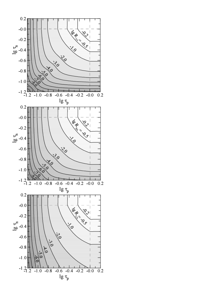
Figure 16: Contours of constant reduction factors $R^{\rm(D)}$ of the direct Urca process in the presence of neutron and proton superfluidities AA, BA and CA (Yakovlev et al. 1999b). The curves are labeled by the values $\lg R^{\rm(D)}$. In the region $\tau_{n}\geq 1$ and $\tau_{p}\geq 1$, neutrons and protons are normal and $R^{\rm(D)}=1$. In the region $\tau_{n}<1$, $\tau_{p}\geq 1$, where only neutrons are superfluid, and in the region $\tau_{n}\geq 1$, $\tau_{p}<1$, where only protons are superfluid, $R^{\rm(D)}$ depends on only one parameter, either $\tau_{n}$ or $\tau_{p}$. In the region $\tau_{n}<1,\;\tau_{p}<1$, both neutrons and protons are superfluid.

Figure 16 shows the contours of $R^{\rm(D)}_{\rm AA}\!=\,$const versus $\tau_{1}=T/T_{c1}$ and $\tau_{2}=T/T_{c2}$. The behavior of $R^{\rm(D)}_{\rm AA}$ at $\tau_{1}^{2}+\tau_{2}^{2}\ll 1$, where both superfluidities are strong, is of special interest. In this case one can obtain an approximate relationship (Lattimer et al. 1991; Levenfish and Yakovlev 1994b)

$$R^{\rm(D)}_{12}\sim\min\left(R^{\rm(D)}_{1}\!,\,R^{\rm(D)}_{2}\right)\,,$$ (204)

where $R^{\rm(D)}_{1}$ and $R^{\rm(D)}_{2}$ are the reduction factors for either type of superfluidity. Roughly speaking, this means that $R^{\rm(D)}_{12}\sim\exp(-\Delta/T)$, where $\Delta$ is the largest of the two gaps, $\Delta_{1}$ and $\Delta_{2}$, since it is the largest gap that opens the process with respect to energy conservation. Accordingly, the factor $R^{\rm(D)}_{12}$ is mainly determined by the stronger superfluidity. The presence of the second, weaker superfluidity affects $R^{\rm(D)}_{12}$, but not to a great extent.

Using Eq. (196), it is not difficult to evaluate $R^{\rm(D)}$ for cases BA and CA, in which the protons undergo singlet-state pairing while the neutrons undergo triplet-state pairing. The calculation is reduced to the one-dimensional integration in Eq. (196) of the quantity $J(y_{1},y_{2})$ fitted by Eqs. (202) and (203). The results for any $T$, $T_{c1}$ and $T_{c2}$ are shown in Fig. 16. The dependence of $R^{\rm(D)}_{\rm BA}$ and $R^{\rm(D)}_{\rm CA}$ on $\tau_{1}$ and $\tau_{2}$ is similar to the dependence of $R^{\rm(D)}_{\rm AA}$, shown in the same figure, but now $R^{\rm(D)}(\tau_{1},\tau_{2})\neq R^{\rm(D)}(\tau_{2},\tau_{1})$. The approximate expression (204) is also valid in these cases (Levenfish and Yakovlev 1994b). Since superfluidity C reduces the neutrino emission much weaker than superfluidities A or B, in the case CA with $v_{1}\gg 1$ the transition from the one dominating superfluidity to the other takes place at $v_{2}\sim\ln v_{1}$. Moreover, for $v_{1}\;\raise 1.29167pt\hbox{$>$\kern-7.5pt\raise-4.73611pt\hbox{$\sim$}}\;v_{2}\gg 1$ the factor $R^{\rm(D)}_{\rm CA}$ appears to be much larger than $R^{\rm(D)}_{\rm AA}$ or $R^{\rm(D)}_{\rm BA}$. Accordingly, the lines of constant $R_{\rm CA}$ are lower than the corresponding contours of $R_{\rm AA}$ or $R_{\rm BA}$ (cf. Figs. 15 and 16).

For not very strong superfluidities BA, with $\sqrt{v_{1}^{2}+v_{2}^{2}\,}\;\raise 1.29167pt\hbox{$<$\kern-7.5pt\raise-4.73611pt\hbox{$\sim$}}\;5$, the reduction factor is fitted by

$$R^{\rm(D)}_{\rm BA}=\frac{10^{4}-2.839\,v_{2}^{4}-5.022\,v_{1}^{4}}{10^{4}+757.0\,v_{2}^{2}+1494\,v_{1}^{2}+211.1\,v_{2}^{2}v_{1}^{2}+0.4832\,v_{2}^{4}v_{1}^{4}}.$$ (205)

In the case of not too strong superfluidities CA, with $\sqrt{v_{1}^{2}+v_{2}^{2}\,}\;\raise 1.29167pt\hbox{$<$\kern-7.5pt\raise-4.73611pt\hbox{$\sim$}}\;10$, the fit is:

$$R^{\rm(D)}_{\rm CA} = 10^{4}\times\left(10^{4}+793.9\,v_{2}^{2}+457.3\,v_{1}^{2}+66.07\,v_{2}^{2}v_{1}^{2}+2.093\,v_{1}^{4}+\right.$$ (206)

$$+ \left.0.3112\,v_{2}^{6}+1.068\,v_{2}^{4}v_{1}^{2}+0.01536\,v_{2}^{4}v_{1}^{4}+0.006312\,v_{2}^{6}v_{1}^{2}\right)^{-1}\,.$$

If $v_{1}=0$ or $v_{2}=0$, the above fits agree with Eqs. (199). The tables of $R^{\rm(D)}_{\rm BA}$ and $R^{\rm(D)}_{\rm CA}$, as well as the asymptotes of these factors in the limit of strong superfluidity, are given in Levenfish and Yakovlev (1994b).

Before publication of the above results (Levenfish and Yakovlev 1993, 1994b), as far as we know, the only simulation of the fast neutron star cooling with the account of superfluidity of neutrons and protons was carried out by Van Riper and Lattimer (1993). They used a simplified reduction factor, $R^{\rm(D)}_{12}=R^{\rm(D)}_{1}R^{\rm(D)}_{2}$, which strongly overestimates the effect of superfluidity.

(c) Other direct Urca processes

We have discussed the superfluid reduction of the nucleon direct Urca process only as an example. The same formulae are valid for any baryon direct Urca process [processes (I) in Table 2, Sect. 3.3] involving electrons or muons and the two baryon species, one of which undergoes singlet pairing. Thus, the presented results are sufficient to describe the superfluid reduction of all reactions with hyperons, since hyperon pairing is expected to be of singlet type (Sect. 1.2).

The reduction of the emissivity in the case of both particles undergoing triplet pairing has not yet been studied, to the best of our knowledge. It would also be interesting to analyze the effects of the triplet-state superfluidity which is a coherent superposition of states with the different projections $m_{J}$ of the total angular momentum of the pair on the quantization axis.

We expect that the above formalism can also be used for a qualitative description of the superfluid reduction of the leading direct-Urca-type reactions in the hypothetic exotic pion condensed or kaon condensed matter (Table 3, Sect. 3.8). In these cases we recommend to use the factor $R^{\rm(D)}_{\rm AA}$, given by Eq. (202) as a function of the superfluid gap parameters, $v_{1}$ and $v_{2}$, and calculate these parameters for the appropriate critical temperatures of the quasiparticle species $\tilde{n}$ and $\tilde{p}$, provided the superfluidities of these quasiparticles can be regarded as independent. This would reflect one of the similarity criteria formulated in Sect. 4.6.

In addition, we expect that similar formalism can be used to study direct Urca processes in quark matter (Sect. 3.8) with superfluidity of like and unlike quarks (Sect. 1.2). In the latter case the critical temperature may be so high, $T_{c}\;\raise 1.29167pt\hbox{$<$\kern-7.5pt\raise-4.73611pt\hbox{$\sim$}}\;50$ MeV, that the superfluidity reduces the direct Urca emissivity to negligibly small level.

4.4 Modified Urca processes in superfluid matter

In this section we analyze superfluid reduction of the modified Urca processes [processes (II) from Table 2, Sect. 3.4]. As an example, we consider the nucleon modified Urca processes involving electrons, Eqs. (125) and (126), but our analysis will actually be more general (see below). Like for the direct Urca process, it is based on the phase-space decomposition and therefore is rather insensitive to the details of the strong interaction model. We adopt the traditional assumption that proton superfluidity is of type A, while neutron superfluidity is of type B. Our results will also be valid for neutron pairing of type A (at $\rho\;\raise 1.29167pt\hbox{$<$\kern-7.5pt\raise-4.73611pt\hbox{$\sim$}}\;\rho_{0}$), as will be mentioned later. Reduction of modified Urca reactions by neutron pairing of type C has not been considered so far. We follow the consideration of Yakovlev and Levenfish (1995).

(a) Reduction factors

Reduction factors $R^{({\rm M}n)}$ and $R^{({\rm M}p)}$ of the neutron and proton branches of modified Urca process can be derived in the same manner as for the direct Urca process (Sect. 4.3) from the phase-space decomposition. In analogy with the direct Urca process, we include the effects of superfluidity by introducing the superfluid gaps into the nucleon dispersion relations. Generally, the reduction factors are given by

$$R^{({\rm M}\!N)}=J_{N}/(I_{N0}A_{N0}),$$ (207)

where $I_{N0}$ and $A_{N0}$ are the energy and angular integrals in the non-superfluid matter, given by Eqs. (129), (131) and (141), and

$$J_{N}=4\pi\int\prod_{j=1}^{5}{\rm d}\Omega_{j}\;\int_{0}^{\infty}{\rm d}x_{\nu}\,x_{\nu}^{3}\left[\prod_{j=1}^{5}\int_{-\infty}^{+\infty}{\rm d}x_{j}\,f(z_{j})\right]\delta\left(x_{\nu}-\sum_{j=1}^{5}z_{j}\right)\delta\left(\sum_{j=1}^{5}{\bf{p}}_{j}\right),$$ (208)

where $z_{j}$ is the same as in Eq. (197) ($j\leq 4$), and $z_{5}=x_{5}=x_{e}$ for the electron.

Equation (208) enables one to calculate the reduction factors $R^{({\rm M}n)}$ and $R^{({\rm M}p)}$ as function of $T$, $T_{cn}$ and $T_{cp}$. Below we present the results for proton superfluidity of type A and normal neutrons, as well as for neutron superfluidity of type B and normal protons. The behavior of $R^{({\rm M}n)}$ and $R^{({\rm M}p)}$ under the combined effect of the $n$ and $p$ superfluids is discussed in Sect. 4.6.

(b) Singlet-state proton pairing

Since the singlet-state gap is isotropic, the angular and energy integrations in Eq. (208) are decomposed and the angular integration remains the same as in the non-superfluid matter.

Just as in the case of direct Urca process, the reduction factors of the neutron and proton branches of modified Urca process, $R_{p{\rm A}}^{({\rm M}n)}$ and $R_{p{\rm A}}^{({\rm M}p)}$, can be expressed in terms of the dimensionless energy gap $v_{p}=v_{\rm A}=v$; hereafter the subscripts in $R^{({\rm M}\!N)}$ indicate the superfluid particle species and superfluidity type. Clearly, $R_{p{\rm A}}^{({\rm M}n)}=1$ and $R_{p{\rm A}}^{({\rm M}p)}=1$ for $T\geq T_{cp}$ ($v_{\rm A}=0$). In the case of strong superfluidity ($T\ll T_{cp}$, $v_{\rm A}\to\infty$), the asymptotes of the two factors are obtained in the same manner as in Sect. 4.3

$$R_{p{\rm A}}^{({\rm M}n)} = {72\sqrt{2\pi}\over 11513\pi^{8}}\,v^{7.5}\exp(-v)={1.166\times 10^{-4}\over\tau^{7.5}}\exp\left(-{1.764\over\tau}\right)\,,$$ (209)

$$R_{p{\rm A}}^{({\rm M}p)} = {120960\over 11513\pi^{8}}\,\xi\,v^{7}\exp(-2v)={0.00764\over\tau^{7}}\exp\left(-{3.528\over\tau}\right),$$ (210)

where $\tau=T/T_{cp}$ and $\xi=0.130$.

Yakovlev and Levenfish (1995) calculated $R_{p{\rm A}}^{({\rm M}n)}$ and $R_{p{\rm A}}^{({\rm M}p)}$ for intermediate $v$ and fitted the results by the analytic expressions, which reproduced the asymptotes in the limit of $v\to\infty$ and obeyed the condition $R^{({\rm M}\!N)}(0)=1$:

$$R_{p{\rm A}}^{({\rm M}n)}\! = \!{a^{7.5}+b^{5.5}\over 2}\exp\left(3.4370-\sqrt{(3.4370)^{2}+v^{2}}\,\right),$$ (211)

$$a\! = \!0.1477+\sqrt{(0.8523)^{2}+(0.1175\,v)^{2}},\quad b=0.1477+\sqrt{(0.8523)^{2}+(0.1297\,v)^{2}};\hskip 14.22636pt$$

$$R_{p{\rm A}}^{({\rm M}p)}\! = \!\left[0.2414\!+\!\sqrt{(0.7586)^{2}\!+\!(0.1318\,v)^{2}}\right]^{7}\exp\left(5.339\!-\!\sqrt{(5.339)^{2}+(2v)^{2}}\,\right).$$ (212)

Equations (211) and (212), together with (188), fully determine the dependence of $R_{p{\rm A}}^{({\rm M}n)}$ and $R_{p{\rm A}}^{({\rm M}p)}$ on $\tau$.

The above results are valid also for the singlet-state superfluidity of neutrons. Evidently, in that case one should set $v_{n}=v_{\rm A}$, and

$$R_{n\rm A}^{({\rm M}p)}(v_{\rm A})=R_{p{\rm A}}^{({\rm M}n)}(v_{\rm A}),\quad R_{n\rm A}^{({\rm M}n)}(v_{\rm A})=R_{p{\rm A}}^{({\rm M}p)}(v_{\rm A}).$$ (213)

Wolf (1966) and Itoh and Tsuneto (1972) were the first to consider the reduction factor $R_{n\rm A}^{({\rm M}n)}=R_{p{\rm A}}^{({\rm M}p)}$ of the neutron branch of modified Urca process by the singlet-state neutron superfluidity. Note that Itoh and Tsuneto analyzed only the asymptote (210). In both papers the same asymptote (210) was obtained but with different numerical factors $\xi$. Wolf (1966) found $\xi=0.123$, while Itoh and Tsuneto (1972) obtained $\xi=\pi/15\approx 0.209$. Recently, $R_{n\rm A}^{({\rm M}n)}$ was independently calculated by Pizzochero (1998) under the artificial assumption that the superfluid gap is temperature-independent. His results can be described by the factor $R_{n\rm A}^{({\rm M}n)}(v_{\rm A})$ given above with $v_{\rm A}=1.764/\tau$.

(c) Triplet-state neutron pairing

In this case the neutron gap is anisotropic. The proton branch of modified Urca process is analyzed easily since the only one superfluid particle is involved. The expression for $R_{n{\rm B}}^{({\rm M}p)}$ reduces to a one-dimensional integral over the angle $\vartheta_{n}$ (between neutron momentum and quantization axis) of factor $R_{p{\rm A}}^{({\rm M}n)}(v)$ fitted by Eq. (211). Argument $v_{\rm A}$ in the latter expression should formally be replaced by $y_{\rm B}=v_{\rm B}\,(1+3\,\cos^{2}\vartheta)^{1/2}$ in accordance with Eq. (187) (Sect. 4.2). It is evident that $R_{n{\rm B}}^{({\rm M}p)}(v)=1$ for $v=v_{\rm B}=0$. In the limit $v\to\infty$ one can use the asymptote (209) in the integrand. Then for $T\ll T_{cn}$ ($v\gg 1$), according to Yakovlev and Levenfish (1995),

$$R_{n{\rm B}}^{({\rm M}p)}={72\over 11513\,\pi^{7}\sqrt{3}}\,v^{7}\exp(-v)={3.99\times 10^{-6}\over\tau^{7}}\exp\left(-{1.188\over\tau}\right)\,,$$ (214)

where $\tau=T/T_{cn}$. The same authors calculated also $R_{n{\rm B}}^{({\rm M}p)}$ for intermediate values of $v$ and fitted the results by the analytic expression:

$$R_{n{\rm B}}^{({\rm M}p)} = {a^{7}+b^{5}\over 2}\exp\left(2.398-\sqrt{(2.398)^{2}+v^{2}}\,\right),$$ (215)

$$a = 0.1612+\sqrt{(0.8388)^{2}+(0.1117\,v)^{2}},\quad b=0.1612+\sqrt{(0.8388)^{2}+(0.1274\,v)^{2}}.$$

Figure 17: Reduction factors of various neutrino emission processes by superfluidity of neutrons or protons versus $T/T_{c}$ (Yakovlev et al. 1999b). Curves 1 show reduction of the $p$-branch of the modified Urca process (solid line) and the direct Urca process (dashed line) by neutron superfluidity of type B. Curves 2 correspond to reduction of the $n$-branch of the modified Urca (solid line) and the direct Urca (dashed line) by proton superfluidity of type A. Dot-and-dash lines 5, 6 and the solid line 3 refer to the $np$, $pp$-scattering and $p$-branch of the modified Urca processes, respectively, for the same proton superfluidity. Solid line 4 is the asymptote of the reduction factor for the $n$-branch of the modified Urca process due to neutron superfluidity of type B.

Exact calculation of $R_{n{\rm B}}^{({\rm M}n)}$ of the neutron branch of modified Urca process by the triplet-state neutron superfluidity for intermediate values of $v$ is complicated; an approximate expression will be given in Sect. 4.6. Here we present only the asymptote of $R_{n{\rm B}}^{({\rm M}n)}$ in the limit $\tau\ll 1$

$$R_{n{\rm B}}^{({\rm M}n)}\!=\!{120960\over 11513\pi^{8}}\;{2\over 3\sqrt{3}}\;\xi\,v^{6}\exp(-2v)={1.56\times 10^{-4}\over\tau^{6}}\exp\left(-{2.376\over\tau}\,\right).$$ (216)

In this case, as for the proton reaction involving superfluid protons (210), the effect of superfluidity is very strong: the exponent argument in $R_{n{\rm B}}^{({\rm M}n)}$ contains the doubled gap. This is because the three neutrons participating in the reaction belong to the superfluid component of matter. Two of them have positive energies [$z\gg 1$, $f(z)\approx{\rm e}^{-z}$] while the third one has negative energy [$z<0$, $f(z)\approx 1$].

Figure 18: Same as in Fig. 17, but versus dimensionless gap parameter (Yakovlev et al. 1999b).

The dependence of reduction factors $R_{p{\rm A}}^{({\rm M}n)}$, $R_{p{\rm A}}^{({\rm M}p)}$, $R_{n{\rm B}}^{({\rm M}p)}$, and $R_{n{\rm B}}^{({\rm M}n)}$ on the dimensionless temperature $\tau$ and the dimensionless gap parameter $v$ is plotted in Figs. 17 and 18. For comparison, we present also reduction factors of direct Urca process, $R^{\rm(D)}_{\rm A}$ and $R^{\rm(D)}_{\rm B}$. Let us mention that in the case of the strong neutron superfluidity ($T\ll T_{cn}$) and normal protons the proton branch of modified Urca process becomes much more efficient than the neutron branch (factors ${\rm e}^{-v}$ and ${\rm e}^{-2v}$ in Eqs. (214) and (216)). However in this case the main neutrino emission comes from neutrino bremsstrahlung due to $pp$-scattering, which is not affected by the neutron superfluidity.

(d) Other modified Urca processes

We have considered superfluid reduction of modified Urca processes involving $n$, $p$, and $e$. It is clear that the same reduction factors describe the processes with muons [processes (II.1) with $B=n$ or $p$ from Table 2]. In hyperon matter, they are also valid for all baryon modified Urca processes (II.1)–(II.4) which involve two types of baryons, for instance, $\Lambda\Lambda\to p\Lambda l\bar{\nu}_{l}$, $p\Lambda l\to\Lambda\Lambda\nu_{l}$ [process (II.2) with $B=\Lambda$ and $l=e$ or $\mu$].

Superfluid suppression of the processes involving three different baryons (e.g., $\Lambda\Sigma^{-}\to p\Sigma^{-}l\bar{\nu}_{l}$, $p\Sigma^{-}l\to\Lambda\Sigma^{-}\nu_{l}$) has not been considered yet. If, however, only one beta decaying baryon belongs to the superfluid component, the present results are valid again. For the cases in which two (of the three) baryons are superfluid, one can construct approximate reduction factors using the similarity criteria formulated in Sect. 4.6.

Finally, there are also modified Urca processes (IV) based on muon decay. Their rate has not been determined accurately so far, and their reduction has not been analyzed. However, these processes produce very weak neutrino emission. If they involve a charged baryon as a spectator, they will be suppressed by the baryon superfluidity and will have negligible neutrino emissivity. If they involve an additional lepton (electron or muon), they will not be suppressed at all although they may be slightly affected by the baryon superfluidity through the plasma screening length. Similar effects will be described in the next section with regard to neutrino bremsstrahlung in $ee$ and $ep$ collisions.

4.5 Neutrino bremsstrahlung in superfluid matter

In this section we analyze the effect of superfluidity on neutrino generation in baryon bremsstrahlung processes [reactions (III) from Table 2, Sect. 3.6] and Coulomb bremsstrahlung processes [reactions (V), Sect. 3.7].

(a) Nucleon-nucleon bremsstrahlung

We start with neutrino-pair bremsstrahlung in $nn$, $np$ and $pp$-collisions [reactions (III.1)–(III.3), Table 2 and Sect. 3.6] following the approach of Yakovlev and Levenfish (1995). The general expression for reduction factors $R^{(N\!N)}$ can be obtained in analogy with Urca reactions from phase-space consideration by inserting the superfluid gap in the nucleon dispersion relation.

Consider singlet superfluid A of neutrons or protons. Then the modification of the dispersion relation by superfluidity affects only the energy integral given by Eq. (157). Accordingly the reduction factors take the form:

$$R^{(N\!N)}={945\over 164\pi^{8}}\int_{0}^{\infty}{\rm d}x_{\nu}\;x_{\nu}^{4}\left[\prod_{j=1}^{4}\int_{-\infty}^{+\infty}{\rm d}x_{j}\;f(z_{j})\right]\delta\left(\sum_{j=1}^{4}z_{j}-x_{\nu}\right).$$ (217)

It is clear that $R^{(N\!N)}=1$ for $\tau\geq 1$.

In the case of proton superfluid A suppression factors of $np$ and $pp$ processes, $R^{\,(np)}_{p{\rm A}}$ and $R^{\,(pp)}_{p{\rm A}}$, are reduced to two dimensional integrals which have been calculated numerically. In the limit of strong superfluidity ($\tau\ll 1$, $v=v_{\rm A}\to\infty$) the asymptotes of these factors are:

$$R^{\,(np)}_{p{\rm A}} = {945\over 164\pi^{8}}\,\xi_{1}\,v\exp(-v)={0.910\over\tau}\exp\left(-{1.764\over\tau}\right),$$ (218)

$$R^{\,(pp)}_{p{\rm A}} = {8505\over 41\pi^{6}}\;v^{2}\exp(-2v)={0.671\over\tau^{2}}\exp\left(-{3.528\over\tau}\right),$$ (219)

where $\xi_{1}\approx 849$. These asymptotes as well as numerical values of $R^{\,(np)}_{p{\rm A}}$ and $R^{\,(pp)}_{p{\rm A}}$ calculated for intermediate values of $v$ are described by the fits:

$$R^{\,(np)}_{p{\rm A}} = {1\over 2.732}\left[\,a\exp\left(1.306-\sqrt{(1.306)^{2}+v^{2}}\right)\right.$$ (220)

$$\left.+\;1.732\,b^{7}\exp\left(3.303-\sqrt{(3.303)^{2}+4v^{2}}\right)\right],$$

$$a = 0.9982+\sqrt{(0.0018)^{2}+(0.3815\,v)^{2}},\quad b=0.3949+\sqrt{(0.6051)^{2}+(0.2666\,v)^{2}}\,;$$

and

$$R^{\,(pp)}_{p{\rm A}} = {1\over 2}\left[\,c^{2}\exp\left(4.228-\sqrt{(4.228)^{2}+(2v)^{2}}\right)\right.$$ (221)

$$+\left.d^{7.5}\exp\left(7.762-\sqrt{(7.762)^{2}+(3v)^{2}}\right)\right],$$

$$c = 0.1747+\sqrt{(0.8253)^{2}+(0.07933\,v)^{2}},\quad d=0.7333+\sqrt{(0.2667)^{2}+(0.1678\,v)^{2}}.$$

For the singlet-state neutron pairing, we evidently have

$$R^{\,(np)}_{n\rm A}(v_{\rm A})=R^{\,(np)}_{p\rm A}(v_{\rm A}),\quad R^{\,(nn)}_{n\rm A}(v_{\rm A})=R^{\,(pp)}_{p\rm A}(v_{\rm A}).$$ (222)

Reduction factors $R^{\,(np)}_{p\rm A}$ and $R^{\,(pp)}_{p\rm A}$ are shown in Fig. 17 versus $T/T_{c}$ and in Fig. 18 versus the dimensionless gap parameter $v$. We will discuss these figures and the case of the triplet-state pairing in the next section.

(b) Hyperon bremsstrahlung processes

The results obtained above are independent of the model of strong interaction and can be used not only for nucleon-nucleon bremsstrahlung reactions (III.1)–(III.3) from Table 2 but for all baryon bremsstrahlung reactions (III.1)–(III.10) which involve baryons of one or two types. Reduction of reactions (III.11) and (III.12) involving baryons of four different types has not been considered yet. If, however, only one or two of the four particles belong to superfluid component, one can construct approximate reduction factors using the similarity criteria formulated in Sect. 4.6.

(c) Coulomb bremsstrahlung processes

For non-superfluid matter, these processes [processes (V), Table 2] have been analyzed in Sect. 3.7. Strictly speaking, all these reactions are affected by superfluidity, and the effect is twofold. The first, most significant effect is that the reaction is suppressed by superfluidity of reacting baryons. This effect can be described introducing the superfluid reduction factor in accordance with Eq. (182). Second, superfluidity of charged baryons affects the plasma screening momentum $q_{s}$, given by Eq. (171), and hence the neutrino emissivity $Q_{0}$ itself in Eq. (182). The second effect is much weaker than the first one, but nevertheless noticeable. One can easily show that in superfluid (superconducting) matter, instead of Eq. (171) we have

$$y_{s}^{2}\equiv{q_{s}^{2}\over 4p_{{\rm F}e}^{2}}={e^{2}\over\pi\hbar c}\,\sum_{j}{m_{j}^{\ast}p_{{\rm F}j}\over m_{e}^{\ast}p_{{\rm F}e}}\;D_{j},$$ (223)

where summation is over all charged fermions $j$ in stellar matter, and $D_{j}$ describes superfluid reduction of corresponding plasma screening. For leptons ($e$ or $\mu$) and for charged baryons $j$ at $T\geq T_{cj}$ this reduction is absent and $D_{j}=1$. For singlet-state pairing of charged baryons at $T<T_{cj}$ reduction factor $D_{j}(v_{j})$ is given by (e.g., Gnedin and Yakovlev 1995)

$$D=\left(0.9443+\sqrt{(0.0557)^{2}+(0.1886\,v)^{2}}\right)^{1/2}\exp\left(1.753-\sqrt{(1.753)^{2}+v^{2}}\right),$$ (224)

where $v$ is the dimensionless gap. In the presence of strong superfluidity ($v\gg 1$) the reduction is exponential, and the charged superfluid (superconducting) baryons of species $j$ produce no screening decreasing thus $y_{s}$. However, this decrease is not crucial since there are always electrons (and possibly muons) which are non-superfluid and determine the residual screening momentum in a strongly superconducting matter.

Consider, for instance, neutrino bremsstrahlung in $ep$ collisions [process (V.1) from Table 2 with $l=e$] discussed in Sect. 3.7 for non-superfluid matter. In the presence of superfluidity, its emissivity $Q^{(ep)}$ is given by Eq. (182), $Q^{(ep)}=Q^{(ep)}_{0}\,R^{(ep)}$, where $Q^{(ep)}_{0}$ is formally given by the same Eq. (170) as in the non-superfluid matter but with the parameter $y_{s}$ affected by the superfluidity and determined by Eqs. (223) and (224). Reduction factor $R^{(ep)}$ for this process can be found using phase space decomposition; it coincides (Kaminker and Haensel 1999) with factor $R^{(np)}_{p{\rm A}}$ for $np$ bremsstrahlung, Eq. (220). For instance, in non-superfluid $npe$ matter the main contribution into screening parameter $y_{s}$ comes from the protons, while the contribution from the electrons is several times smaller. When temperature $T$ decreases below $T_{cp}$ the proton superfluidity enhances emissivity $Q^{(ep)}_{0}$ by a factor of several, with respect to its purely non-superfluid value by decreasing $y_{s}$, but reduces full emissivity $Q^{(ep)}$ much stronger owing to the exponential superfluid reduction described by factor $R^{(ep)}$. Similar equations describe the neutrino emissivities due to Coulomb collisions of electrons or muons with all charged baryons [all processes (V.1)–(V.2)].

Another example is neutrino bremsstrahlung due to collisions between leptons [processes (V.3)] which experience no direct superfluid reduction. For instance, consider bremsstrahlung in $ee$ collisions [process (V.3) with $l=e$] which always operates the neutron star cores. Without superfluidity, it has been discussed in Sect. 3.7. Its emissivity $Q^{(ee)}$ is given by Eq. (173) and contains the same screening parameter $y_{s}$. If the baryon superfluidity is switched on, the same equation remains true ($R^{(ee)}\equiv 1$) but the parameter $y_{s}$ becomes reduced in accordance with Eq. (223). This effect enhances $Q^{(ee)}$ over its purely non-superfluid value by a factor of several as discussed above. Therefore, the emissivity of lepton-lepton bremsstrahlung processes shows no superfluid reduction. Although these neutrino reactions are really weak (Table 2) they can be leading neutrino processes in highly superfluid neutron star cores (Sects. 4.8 and 4.10).

The latter statement can be especially true in strange quark matter with pairing of unlike quarks (Sect. 1.2). This pairing may be very strong to lock all the neutrino processes involving quarks. However, strange quark matter is known to contain a small admixture of electrons. Their neutrino bremsstrahlung would dominate.

4.6 Similarity criteria

As we have seen in Chapt. 3 the number of neutrino reactions is large. Calculation of superfluid reduction factors for all reactions is naturally complicated. However, if a high accuracy is not needed, one can avoid the calculation by noticing similarity of the reduction factors for different reactions (Yakovlev and Levenfish 1995, Levenfish and Yakovlev 1996).

Let us demonstrate these similarity criteria for neutrino reaction in $npe$ matter, although analogous formulae can be proposed for hyperonic matter containing muons.

As seen from Figs. 17 and 18, the reduction factors of various processes in $npe$ matter are different. The main difference comes from the exponent arguments in the asymptotes of the reduction factors in the limit of strong superfluidity. An examination of the asymptotes presented in Sects. 4.3 – 4.5 reveals that the exponent argument contains a single gap if one or two reacting particles belong to superfluid component of matter. Under the number of superfluid reacting particles we mean the total number of particles (in the initial and final states of a bremsstrahlung process, in the initial and final states of either direct or inverse reaction of an Urca process) belonging to the superfluid components. For instance, the gap in the exponent argument is doubled if three or four superfluid particles are involved. According to Fig. 18, factor $R^{\,(np)}_{p{\rm A}}$ (two superfluid particles) decreases with the growth of superfluidity strength $v$ much more rapidly than $R_{p{\rm A}}^{({\rm M}n)}$ or $R_{n{\rm B}}^{({\rm M}p)}$ (one superfluid particle). Accordingly, $R^{\,(pp)}_{p{\rm A}}$ (four superfluid particles) decreases faster than $R_{p{\rm A}}^{({\rm M}p)}$ (three superfluid particles). Therefore, superfluid suppression is most strongly affected by the number of superfluid reacting particles. Let us stress that we discuss neutrino reactions of Urca or bremsstrahlung type. The formulated rule must be modified for neutrino emission due to Cooper pairing of nucleons (Sect. 4.7).

At the next step it is important to emphasize that the reduction factors in $npe$ matter for the processes involving one superfluid particle ($R^{\rm(D)}_{\rm A}$, $R_{p{\rm A}}^{({\rm M}n)}$, $R^{\rm(D)}_{\rm B}$, and $R_{n{\rm B}}^{({\rm M}p)}$) are close to one another as functions of the dimensionless gap parameter $v$ (Fig. 18). This enabled Levenfish and Yakovlev (1996) to construct approximate reduction factors for the proton and neutron branches of modified Urca process in the presence of the neutron and proton superfluids:

$$R^{({\rm M}p)}_{\rm BA}(v_{n},v_{p}) \approx {R^{\rm(D)}_{\rm BA}(v_{n},2v_{p})\over R^{\rm(D)}_{\rm B}(v_{n})}\,R_{n{\rm B}}^{({\rm M}p)}(v_{n})\,,$$ (225)

$$R^{({\rm M}n)}_{\rm BA}(v_{n},v_{p}) \approx {R^{\rm(D)}_{\rm BA}(2v_{n},v_{p})\over R^{\rm(D)}_{\rm A}(v_{p})}\,R_{p{\rm A}}^{({\rm M}n)}(v_{p}).$$ (226)

We expect that these factors, as functions of corresponding parameters $v$ (corrected due to the number of superfluid particles) do not differ strongly from reduction factor $R^{\rm(D)}_{\rm BA}(v_{n},v_{p})$ for the direct Urca process. If protons are normal ($v_{p}=0$), then the expression for $R^{({\rm M}p)}_{\rm BA}(v_{n},v_{p})$ becomes exact; if neutron are normal ($v_{n}=0$), factor $R^{({\rm M}n)}_{\rm BA}(v_{n},v_{p})$ is exact. In addition, the approximate factors satisfy the relationships analogous to Eq. (204).

Therefore, new reduction factors $R^{({\rm M}p)}_{\rm BA}(v_{n},v_{p})$ and $R^{({\rm M}n)}_{\rm BA}(v_{n},v_{p})$ are expressed through the factors obtained in Sects. 4.3 and 4.4.

One can also expect similarity of reduction factors for other neutrino reactions. For instance, reduction factor of the neutron branch of modified Urca process, $R_{n{\rm B}}^{({\rm M}n)}$, by a moderate neutron superfluidity ($v\;\raise 1.29167pt\hbox{$<$\kern-7.5pt\raise-4.73611pt\hbox{$\sim$}}\;10$) should not deviate strongly from reduction factor of the proton branch of modified Urca process, $R_{p{\rm A}}^{({\rm M}p)}$, by the proton superfluidity:

$$R_{n{\rm B}}^{({\rm M}n)}\approx R_{p{\rm A}}^{({\rm M}p)}(v_{n}).$$ (227)

Approximate reduction factor $R^{\,(nn)}_{n{\rm B}}$ of $nn$ scattering in the presence of $n$ superfluidity and approximate reduction factor $R^{\,(np)}_{\rm BA}$ of $np$ scattering by neutron and proton superfluidities can be written as

$$R^{\,(nn)}_{n{\rm B}} \approx R^{\,(pp)}_{p{\rm A}}(v_{n})\,,$$ (228)

$$R^{\,(np)}_{\rm BA} \approx {R^{\rm(D)}_{\rm BA}(v_{n},v_{p})\over R^{\rm(D)}_{\rm A}(v_{p})}\,R^{\,(np)}_{p{\rm A}}(v_{p})\,.$$ (229)

In the absence of the neutron superfluidity, Eq. (229) becomes exact.

We can warn the reader once more that the similarity criteria are not exact and it would be interesting to calculate accurately all reduction factors in the future. Nevertheless it is worth to mention that one does not need very accurate values of the neutrino emissivity for simulations of neutron star cooling: some theoretical uncertainties in the emissivity are easily compensated by very small variations of the temperature due to strong temperature dependence of the emissivity.

4.7 Neutrino emission due to Cooper pairing of baryons

In contrast to the neutrino emission processes considered above this process is allowed only in the presence of superfluidity: the superfluidity distorts the baryon dispersion relation near the Fermi surface and opens the reaction

$$B\to B+\nu+\bar{\nu}\,,$$ (230)

where $B$ stands for any baryon (nucleon or hyperon) which belongs to superfluid component of matter. This reaction is forbidden without the superfluid gap by energy-momentum conservation. Thus the process consists in emission of a neutrino pair by a baryon whose energy spectrum contains a gap. However, in theoretical studies, it is convenient to use the formalism of quasi-particles (Sect. 4.2) and treat the process (Flowers et al.  1976) as annihilation of two quasi-baryons $\widetilde{B}$ with nearly antiparallel momenta into a neutrino pair (which may be considered as Cooper pair formation):

$$\widetilde{B}+\widetilde{B}\to\nu+\bar{\nu}.$$ (231)

The reaction is described by the simplest one-vortex four-tail Feynman diagram; it goes via weak neutral currents and produces neutrinos of all flavors.

To be specific, we discuss the reaction involving nucleons (neutrons or protons) and mention hyperonic reactions later. Following Yakovlev et al. (1999a) we outline derivation of the neutrino emissivity due to singlet-state or triplet-state pairing of non-relativistic nucleons. The reaction is described by the Hamiltonian similar to that for ordinary beta decay [Eq. (97), Sect. 3.2]

$$\hat{H}=-{G_{\rm F}\over 2\sqrt{2}}\,\left(c_{V}\,J_{0}l_{0}-c_{A}\,{\bf{J}}{\bf{l}}\right),$$ (232)

where $c_{V}$ and $c_{A}$ are, respectively, the vector and axial-vector constants of neutral hadron currents. For the neutron current, we have (see, e.g., Okun’ 1984) $c_{V}=1$, $c_{A}=g_{A}=1.26$, while for the proton current $c_{V}=4\,\sin^{2}\Theta_{\rm W}-1\approx-0.08$, $c_{A}=-g_{A}$, $\Theta_{\rm W}$ being the Weinberg angle ($\sin^{2}\Theta_{\rm W}=0.23$). Strong difference of $c_{V}$ for neutrons and protons comes from different quark structure of these particles. Furthermore,

$$J_{0}\equiv\hat{\Psi}^{\dagger}\hat{\Psi},\quad{\bf J}\equiv-\hat{\Psi}^{\dagger}{\bf\sigma}\hat{\Psi},\quad l^{\alpha}=\overline{\psi}_{\nu}\gamma^{\alpha}(1+\gamma^{5})\psi_{\nu},$$ (233)

$l^{\alpha}$ being the 4-vector of the neutrino current ($\alpha$=0,1,2,3); other notations are the same as in Sect. 3.2. In the present discussion, as in Sect. 4.3, we use second–quantized quasi-nucleon wave function $\hat{\Psi}$ described in Sect. 4.2, Eq. (190).

Let $p_{\nu}=(\epsilon_{\nu},{\bf{p}}_{\nu})$ and $p^{\prime}_{\nu}=(\epsilon^{\prime}_{\nu},{\bf{p}}^{\prime}_{\nu})$ be 4-momenta of neutrino and antineutrino, respectively, while $p=(\epsilon,{\bf{p}})$ and $p^{\prime}=(\epsilon^{\prime},{\bf{p}}^{\prime})$ be 4-momenta of annihilating quasi-nucleons. Using Golden Rule of quantum mechanics, we can present the neutrino emissivity due to Cooper pairing (CP) as:

$$Q^{\rm(CP)} = \left({G_{\rm F}\over 2\sqrt{2}}\right)^{2}\,{1\over 2}\,{\cal N}_{\nu}\,\int{{\rm d}{\bf{p}}\over(2\pi)^{3}}\;{{\rm d}{\bf{p}}^{\prime}\over(2\pi)^{3}}\;f(\epsilon)f(\epsilon^{\prime})$$ (234)

$$\times\int{{\rm d}{\bf{p}}_{\nu}\over 2\epsilon_{\nu}(2\pi)^{3}}\;{{\rm d}{\bf{p}}^{\prime}_{\nu}\over 2\epsilon^{\prime}_{\nu}(2\pi)^{3}}\;\left[c_{V}^{2}{\cal J}_{00}|l_{0}|^{2}+c_{A}^{2}\,{\cal J}_{jk}l_{j}l_{k}^{\ast}\right]$$

$$\times(2\pi)^{4}\,\delta^{(4)}\left(p+p^{\prime}-p_{\nu}-p^{\prime}_{\nu}\right)\,(\epsilon_{\nu}+\epsilon^{\prime}_{\nu}),$$

where ${\cal N}_{\nu}$=3 is the number of neutrino flavors, and the factor $1/2$ before ${\cal N}_{\nu}$ excludes double counting of the same quasi-nucleon collisions. The integral is taken over the range $(p_{\nu}+p^{\prime}_{\nu})^{2}>0$, where the process is open kinematically; $f(\epsilon)=1/[\exp(\epsilon/T)+1]$, $j,k\,=\,1,2,3$;

$${\cal J}_{00}=\sum_{\eta\eta^{\prime}}\,|(\hat{\Psi}^{+}\hat{\Psi})_{fi}|^{2},\quad{\cal J}_{jk}=\sum_{\eta\eta^{\prime}}\,(\hat{\Psi}^{+}\sigma_{j}\hat{\Psi})_{fi}\,(\hat{\Psi}^{+}\sigma_{k}\hat{\Psi})_{fi}^{\ast}.$$ (235)

Here $i$ stands for an initial state of the quasi-particle system in which the one-particle states $({\bf{p}},\eta)$ and $({\bf{p}}^{\prime},\eta^{\prime})$ are occupied, and $f$ stands for a final state of the system in which the indicated one-particle states are empty.

Integral (234) is simplified using the standard technique. The simplifications imply that nucleons are non-relativistic and strongly degenerate as well as that the process is open kinematically in a small domain of momentum space, where the quasi-nucleon momenta $\bf{p}$ and ${\bf{p}}^{\prime}$ are almost antiparallel. The latter circumstance allows one to take smooth functions ${\cal J}_{00}({\bf{p}},{\bf{p}}^{\prime})$ and ${\cal J}_{jk}({\bf{p}},{\bf{p}}^{\prime})$ out of the integral over ${\rm d}{\bf{p}}^{\prime}$ putting ${\bf{p}}^{\prime}=-{\bf{p}}$. After some transformations the final expression for the neutrino emissivity can be written (in standard physical units) as (Yakovlev et al.  1998, 1999a)

$$Q^{\rm(CP)} = {4G_{\rm F}^{2}m_{N}^{\ast}p_{\rm F}\over 15\pi^{5}\hbar^{10}c^{6}}\,(k_{\rm B}T)^{7}\,{\cal N}_{\nu}\;aF(v)=$$ (236)

$$= 1.170\times 10^{21}\,\left({m_{N}^{\ast}\over m_{N}}\right)\left({p_{\rm F}\over m_{N}c}\right)\,T_{9}^{7}\,{\cal N}_{\nu}\;aF(v)\;\;{\rm erg\;cm^{-3}\;s^{-1}},$$

where $a$ is a numerical factor (see below), and the function $F(v)$, in our standard notations (185), is given by the integral

$$F(v)={1\over 4\pi}\,\int{\rm d}\Omega\,y^{2}\int_{0}^{\infty}\,{z^{4}\,{\rm d}x\over({\rm e}^{z}+1)^{2}},$$ (237)

$v$ being the gap parameter, Eq. (186). The singlet-state gap is isotropic; thus, integration over all orientations of the nucleon momentum at the Fermi surface (over ${\rm d}\Omega$) is trivial and gives $4\pi$. In the triplet case, $F(v)$ contains averaging over positions of a quasi-nucleon on the Fermi surface. Using Eq. (236), one can take into account that $p_{\rm F}/(m_{N}c)\approx 0.353\,(n_{N}/n_{0})^{1/3}$, where $n_{N}$ is the number density of nucleons $N$, $n_{0}=0.16$ fm^-3.

The emissivity $Q^{\rm(CP)}$ depends on superfluidity type through factor $a$ and function $F(v)$. For the singlet-state neutron pairing, $a$ is determined by the only vector constant $c_{V}$: $a_{n\rm A}=c_{V}^{2}=1$. If we used similar expression for the singlet-state pairing of protons, we would obtain a very small factor $a_{p\rm A}=0.0064$, which mean weakness of neutrino emission. Under these conditions, one should take into account relativistic correction to $a$, produced by the axial-vector proton current. Calculating and adding this correction for the singlet-state pairing of protons, Kaminker et al. (1999b) obtained

$$a_{p\rm A}=c_{V}^{2}+c_{A}^{2}\left(v_{{\rm F}p}\over c\right)^{2}\left[\left(\frac{m_{p}^{\ast}}{m_{p}}\right)^{2}+\frac{11}{42}\right]=0.0064+1.59\left(v_{{\rm F}p}\over c\right)^{2}\left[\left(\frac{m_{p}^{\ast}}{m_{p}}\right)^{2}+\frac{11}{42}\right],$$ (238)

where $v_{{\rm F}p}/c=p_{{\rm F}p}/(m_{p}^{\ast}c)$. The relativistic correction appears to be about 10 – 50 times larger than the main non-relativistic term. This enhances noticeably neutrino emission produced by singlet-state proton pairing although it remains much weaker than the emission due to the neutron pairing.

In the case of the triplet-state pairing, $a$ is determined by both, the vector and the axial-vector, constants of neutral hadron currents: $a=a_{N\rm B}=a_{N\rm C}=c_{V}^{2}+2c_{A}^{2}$ (Yakovlev et al. 1999a). For neutron pairing, we obtain $a_{n\rm B}=a_{n\rm C}=4.17$. Notice that in a not very realistic case of triplet pairing of protons we would obtain $a_{p\rm B}=a_{p\rm C}=3.18$. Under such exotic conditions, neutrino emission due to proton pairing would be almost as efficient as the emission due to neutron pairing.

The result for the singlet-state pairing of neutrons, presented above, coincides with that obtained in the pioneering paper by Flowers et al. (1976) (for two neutrino flavors, ${\cal N}_{\nu}=2$). Similar expressions obtained by Voskresensky and Senatorov (1986, 1987) for ${\cal N}_{\nu}=1$ contain an extra factor $(1+3g_{A}^{2})$. In addition, the expression for $Q^{\rm(CP)}$ derived by the latter authors contains a misprint: $\pi^{2}$ in the denominator instead of $\pi^{5}$, although numerical estimate of $Q^{\rm(CP)}$ is obtained with the correct factor $\pi^{5}$. The cases of singlet proton pairing and triplet neutron pairing were analyzed, for the first time, by Yakovlev et al. (1998, 1999a) and Kaminker et al. (1999b).

Let us remind that the values of $c_{V}$, $c_{A}$ and $a$ can be renormalized in dense matter due to in-medium effects. The renormalization is a difficult task which we neglect. However one should bear in mind that the medium effects may be stronger than the relativistic correction to the proton pairing and determine actually $a_{p\rm A}$.

Function $F(v)$, given by Eq. (237), depends on the only argument $v$, the gap parameter. Using Eq. (237) one can easily obtain the asymptote of this function and calculate its dependence on $\tau=T/T_{c}$ for superfluids A, B and C in analogy with calculations presented in Sects. 4.3–4.5. This was done by Yakovlev et al. (1998, 1999a).

In a small vicinity of $T\approx T_{c}$, in which $v\ll 1$ and $\tau\to 1$, these authors obtained:

$$F_{\rm A}(v) = 0.602\,v^{2}=5.65\,(1-\tau),$$

$$F_{\rm B}(v) = 1.204\,v^{2}=4.71\,(1-\tau),$$

$$F_{\rm C}(v) = 0.4013\,v^{2}=4.71\,(1-\tau).$$ (239)

For low temperatures $T\ll T_{c}$ (i.e., for $v\gg 1$) the asymptotes of $F(v)$ are

$$F_{\rm A}(v) = {\sqrt{\pi}\over 2}\,v^{13/2}\,\exp(-2v)={35.5\over\tau^{13/2}}\,\exp\left(-\frac{3.528}{\tau}\right),$$

$$F_{\rm B}(v) = {\pi\over 4\sqrt{3}}\,v^{6}\,\exp(-2v)={1.27\over\tau^{6}}\,\exp\left(-\frac{2.376}{\tau}\right),$$

$$F_{\rm C}(v) = {50.03\over v^{2}}=12.1\,\tau^{2}.$$ (240)

Neutrino emission due to nucleon pairing differs from other neutrino reactions: first, is has a temperature threshold, $T=T_{c}$; second, its emissivity is a nonmonotonic function of temperature. The emissivity grows rapidly with decreasing $T$ just after superfluidity onset, reaches maximum and decreases. According to Eq. (240), a strong superfluidity reduces considerably the emissivity just as it reduces direct Urca process and other standard reactions (Sects. 4.3–4.5): the reduction is exponential if the gap is nodeless (cases A and B) and it is power-law otherwise (case C). For cases A and B the asymptotes (240) contain the doubled gap in the exponent. This is natural because our process consists actually of nucleon transition from a state with the energy above the Fermi level into a state with the energy below the Fermi level. The minimum separation of the energies of the initial and final states is given by the doubled gap.

The asymptotes (239) and (240), as well as numerical values of $F(v)$ for intermediate $v$, are fitted by the simple expressions (Yakovlev et al.  1998, 1999a)

$$F_{\rm A}(v) = (0.602\,v^{2}+0.5942\,v^{4}+0.288\,v^{6})\,\left(0.5547+\sqrt{(0.4453)^{2}+0.0113\,v^{2}}\right)^{1/2}$$

$$\times\,\exp\left(-\sqrt{4\,v^{2}+(2.245)^{2}}+2.245\right),$$

$$F_{\rm B}(v) = {1.204\,v^{2}+3.733\,v^{4}+0.3191\,v^{6}\over 1+0.3511\,v^{2}}\,\left(0.7591+\sqrt{(0.2409)^{2}+0.3145\,v^{2}}\right)^{2}$$

$$\times\,\exp\left(-\sqrt{4\,v^{2}+(0.4616)^{2}}+0.4616\right),$$

$$F_{\rm C}(v) = {0.4013\,v^{2}-0.043\,v^{4}+0.002172\,v^{6}\over 1-0.2018\,v^{2}+0.02601\,v^{4}-0.001477\,v^{6}+0.0000434\,v^{8}}.$$ (241)

Figure 19: Temperature dependence of the neutrino emissivity due to Cooper pairing of neutrons for $\rho=2\times 10^{14}$ g cm^-3 and $T_{cn}=10^{9}$ K for superfluidity A (solid line), B (dashes) and C (dots); from Yakovlev et al. (1999b).

Equations (236) and (241) enable one to calculate easily neutrino emissivity $Q^{\rm(CP)}$ due for superfluidity A, B and C.

Figure 19 shows temperature dependence of the emissivity $Q^{\rm(CP)}$ due to neutron pairing in a neutron star core for $\rho=2\times 10^{14}$ g cm^-3. We adopted the moderate equation of state of matter described in Sect. 5.1. The effective nucleon masses are set equal to $m_{N}^{\ast}=0.7\,m_{N}$, and the critical temperature is $T_{cn}=10^{9}$ K. The density of study is typical for transition between the single-state pairing and the triple-state one (Sect. 1.2). Thus, different models of nucleon–nucleon interaction may lead to different neutron superfluidity type, and we show the curves for all three superfluidity types considered above.

When the temperature falls down below $T_{cn}$, the neutrino emissivity produced by the Cooper pairing sharply increases. The main neutrino energy release takes place in the temperature interval $0.2\,T_{cn}\;\raise 1.29167pt\hbox{$<$\kern-7.5pt\raise-4.73611pt\hbox{$\sim$}}\;T\;\raise 1.29167pt\hbox{$<$\kern-7.5pt\raise-4.73611pt\hbox{$\sim$}}\;0.96\,T_{cn}$, with the maximum at $T\approx 0.8\,T_{cn}$. The emissivity may be sufficiently high, compared with or even larger than the emissivity of modified Urca process in non-superfluid matter (Sect. 3.4). The reaction may be noticeable even in the presence of direct Urca process in the inner neutron star core if the direct Urca process is strongly reduced by the proton superfluidity (see below). Neutrino emission due to pairing of neutrons may also be significant in inner neutron star crusts (Sect. 2.8).

Equations similar to (236) describe neutrino emission due to Cooper pairing of hyperons. In this case $m_{N}^{\ast}$ should be replaced by the effective baryon mass $m_{B}^{\ast}$, and $p_{\rm F}$ should be treated as the baryon Fermi momentum, while $F(v)$ is given by the same Eq. (241); the case of singlet-state hyperon pairing is most important for applications. The required values of $a$ are listed in Yakovlev et al. (1999a). For instance, in $npe\mu\Lambda\Sigma^{-}$ matter it would be reasonable to assume the singlet state pairing of $\Sigma^{-}$, and $\Lambda$ hyperons (e.g., Balberg and Barnea 1998). For $\Sigma^{-}$, Yakovlev et al. (1999a) yield $a_{\Sigma}=(2-4\sin^{2}\Theta_{\rm W})^{2}=1.17$. The situation with $\Lambda$-hyperons is similar to that with protons: one formally has $a_{\Lambda}=0$ in the non-relativistic approximation including the vector neutral currents but one obtains small finite value of $a_{\Lambda}$ by including either non-relativistic correction or in-medium effects. In any case one can expect that neutrino emission due to pairing of $\Lambda$ particles is very weak. Note that similar formalism can be used to describe neutrino emission due to pairing of quarks in quark matter (Sect. 1.2). Pairing of unlike quarks (if allowed) with very large superfluid gaps would occur just at the neutron star birth (at the proto-neutron-star stage) producing a very strong neutrino outburst.

4.8 Leading reactions in superfluid cores

Now we are ready to summarize the results of Sects.  4.3– 4.7 and compare the neutrino emissivities of different reactions in superfluid cores of neutron stars.

For illustration, we restrict ourselves to $npe$ matter, and use the same moderate equation of state in the neutron star core as in the cooling simulations presented in Chapt. 5 with the nucleon effective masses $m_{N}^{\ast}=0.7\,m_{N}$. We assume further the neutron pairing of type B and the proton pairing of type A. We follow consideration of Yakovlev et al. (1999b).

Figure 20: Temperature dependence of neutrino emissivity in different reactions for neutron superfluidity B with $T_{cn}=8\times 10^{8}$ K and proton superfluidity A with $T_{cp}=4\times 10^{9}$ K at $\rho=2\,\rho_{0}$ (standard neutrino reactions, left panel) and $\rho=5\,\rho_{0}$ (direct Urca process is allowed, right panel). Dot-and-dash line shows the emissivity due to Cooper pairing (CP) of neutrons plus protons; solid line presents the total emissivity. On the left panel the dashed line (M) gives the total emissivity of two branches of modified Urca process; the dotted line (NN) exhibits total bremsstrahlung emissivity in $nn$, $np$ and $pp$ collisions. The right panel: dashed line (D) corresponds to direct Urca process.

Figures 20 show temperature dependence of the neutrino emissivities in different reactions for $T_{cn}=8\times 10^{8}$ K and $T_{cp}=4\times 10^{9}$ K. The left panel corresponds to $\rho=2\rho_{0}$ and can be compared with analogous Fig. 11 for non-superfluid matter. The direct Urca process is forbidden at this density being allowed at $\rho_{\rm crit}=4.64\,\rho_{0}=1.298\times 10^{15}$ g cm^-3, for the given equation of state. In the absence of the neutron superfluidity ($T>T_{cn}$) the most efficient is modified Urca process. If, however, the temperature decreases from $T=T_{cn}$ to $T\approx 10^{8.8}$ K, the total neutrino emissivity increases by about two orders of magnitude due to neutrino emission produced by Cooper pairing of neutrons. Thus the appearance of superfluidity may accelerate neutron star cooling instead of slowing it.

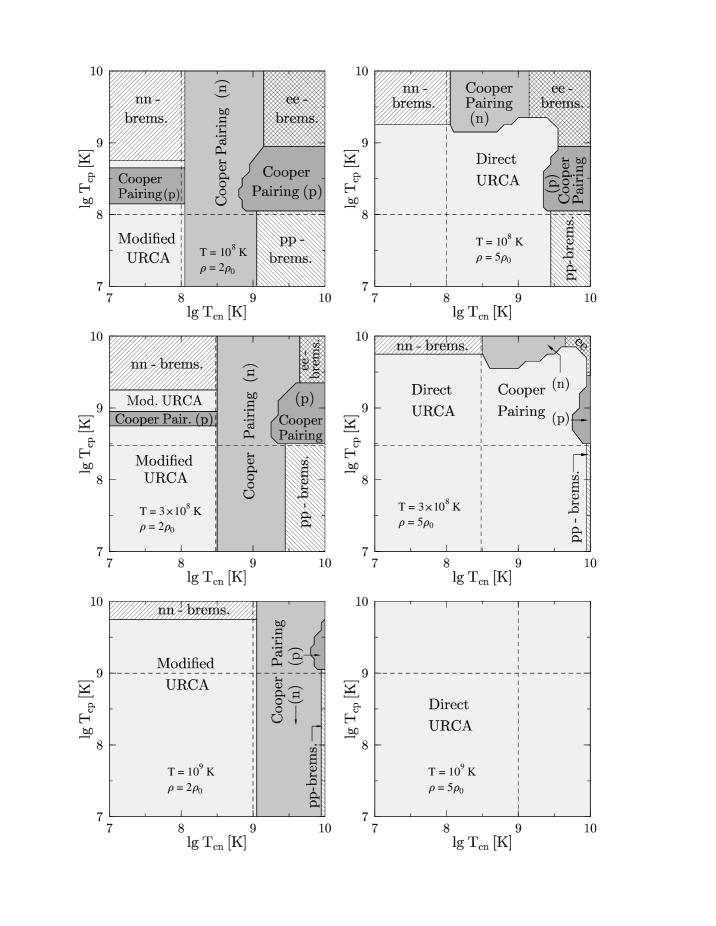
Figure 21: Regions of $T_{cn}$ (superfluidity of type B) and $T_{cp}$ (type A), in which different neutrino reactions dominate at $T=10^{9}$, $3\times 10^{8}$ and $10^{8}$ K (horizontal and vertical dashed lines) in matter of density $\rho=2\,\rho_{0}$ (standard cooling) and $\rho=5\,\rho_{0}$ (enhanced cooling); from Yakovlev et al. (1999b).

The right panel of Fig. 20 corresponds to a denser matter, $\rho=5\rho_{0}$, where the powerful direct Urca process operates. In this case, the neutrino emissivity is actually determined by the two processes, direct Urca and Cooper pairing of nucleons. The direct Urca process dominates at $T\;\raise 1.29167pt\hbox{$>$\kern-7.5pt\raise-4.73611pt\hbox{$\sim$}}\;3\times 10^{8}$ K. With further decrease of $T$, the Urca and nucleon-nucleon bremsstrahlung processes are reduced so strongly that Cooper-pairing neutrino emission becomes dominant.

As discussed in Chapt. 3, neutrino emission from a non-superfluid neutron star core is mainly determined by a single, most powerful neutrino emission mechanism: direct Urca process for the enhanced (fast) cooling, or modified Urca process for the standard (slow) cooling. However, as seen from Fig. 20, superfluidity violates this “simplicity”. Different neutrino mechanisms can dominate at different cooling stages depending on $T$, $T_{cn}$, $T_{cp}$, and $\rho$.

Figures 21 show which neutrino mechanisms dominate for different $T_{cn}$ and $T_{cp}$ in $npe$ matter. In addition to neutrino processes which involve nucleons we have included also neutrino bremsstrahlung in electron–electron collisions (Sect. 4.5). This mechanism is weak and, as a rule, it can be neglected in cooling simulations. Three left Figs. 21 illustrate standard cooling at $\rho=2\,\rho_{0}$ for the three values of the internal stellar temperatures: $10^{8}$, $3\times 10^{8}$ and $10^{9}$ K; three right figures correspond to enhanced cooling at $\rho=5\,\rho_{0}$ for the same $T$. The chosen values of $T$ cover the region most interesting for practice. Our calculations show that topology of the figures varies only slightly with $\rho$ as long as $\rho$ does not cross the threshold value $\rho=\rho_{\rm crit}$. Therefore, the presented figures reflect adequately the efficiency of all neutrino processes in the cores of cooling neutron stars. One can see that, in the presence of superfluidity, many different mechanisms can dominate in certain parameter ranges.

Notice that if the direct Urca process is open, the modified Urca is always insignificant. In the presence of the neutron superfluidity alone, neutrino bremsstrahlung in $pp$ collisions becomes the main mechanism at $T\ll T_{cn}$ being unaffected by the neutron superfluidity. In the presence of the proton superfluidity alone, neutrino bremsstrahlung in $nn$ collisions dominates at $T\ll T_{cp}$. Cooper-pairing neutrino emission of neutrons exceeds neutrino emission in other reactions for $T\;\raise 1.29167pt\hbox{$<$\kern-7.5pt\raise-4.73611pt\hbox{$\sim$}}\;10^{9}$ K and for not too strong neutron superfluidity ($0.12\;\raise 1.29167pt\hbox{$<$\kern-7.5pt\raise-4.73611pt\hbox{$\sim$}}\;T/T_{cn}\;\raise 1.29167pt\hbox{$<$\kern-7.5pt\raise-4.73611pt\hbox{$\sim$}}\;0.96$). This parameter range is very interesting for applications. Neutrino emission due to Cooper pairing of neutrons is also significant in a hotter matter (at earlier cooling stages), when $T\;\raise 1.29167pt\hbox{$>$\kern-7.5pt\raise-4.73611pt\hbox{$\sim$}}\;10^{9}$ K, but in a narrower temperature range near $T\approx 0.8\,T_{cn}$, or in the presence of the proton superfluidity. Although neutrino production in proton pairing is much weaker, it can also dominate. Neutrino emission due to pairing of neutrons and protons can dominate in rapid cooling as well in the cases in which the nucleons of one species are strongly superfluid while the other ones are moderately superfluid. Very strong superfluidities of neutrons and protons (upper right corners of the figures) switch off all neutrino processes involving nucleons. As a result, neutrino bremsstrahlung in electron–electron collisions, which is practically unaffected by superfluidity, becomes dominant producing residual neutrino emissivity from highly superfluid neutron star cores. This case is discussed further in Sect. 4.10.

4.9 Direct Urca process in strong magnetic fields

Now we are turning from the effects of superfluidity to the effects of strong magnetic fields on neutrino emission from neutron star cores. In this section we consider the simplest and most powerful direct Urca process in a non-superfluid but strongly magnetized core. We will discuss the basic nucleon direct Urca process (111) but the same technique can be used to analyze other direct Urca processes involving hyperons and muons.

Beta–decay and related reactions in strong magnetic fields have been studied since late 1960’s (e.g., Canuto and Chiu 1971, Dorofeev et al. 1985, Lai and Shapiro 1991, and references therein). However, these results have been obtained under various simplified assumptions (constant matrix elements, non–degenerate nucleons, etc.); they do not give explicitly the emissivity of direct Urca process in neutron star cores. Works on the subject have been appearing later from time to time with rather contradictory results.

From our point of view, the problem was solved with considerable accuracy by Baiko and Yakovlev (1999). We summarize their results below. We mainly concentrate on the realistic case, in which the magnetic field is not extremely high (although still high, $B\;\raise 1.29167pt\hbox{$<$\kern-7.5pt\raise-4.73611pt\hbox{$\sim$}}\;3\times 10^{16}$ G), and charged particles populate many Landau levels. We will mention also the case of superstrong fields.

(a) Quantum formalism

First, we outline derivation of the neutrino emissivity of direct Urca process valid at any magnetic field $B\ll 10^{20}$ G (at higher fields protons become relativistic). We consider neutrino emission in a pair of reactions (111) under the conventional assumption that reacting electrons are relativistic, while protons and neutrons are nonrelativistic. Calculations are similar to those in Sects. 3.2 and 3.3. The interaction Hamiltonian is that for the ordinary beta decay, Eq. (97). The rate of transition from an initial state $i$ to a final state $f$ is again given by Fermi Golden Rule which can be schematically written as $W_{i\to f}=2\pi|H_{fi}|^{2}\delta(\epsilon_{n}-\epsilon_{p}-\epsilon_{e}-\epsilon_{\nu})$, cf with Eq. (102). We will use the wave functions of electrons and protons in a constant quantizing magnetic field ${\bf B}=(0,0,B)$ (the Landau states) choosing the Landau gauge of the vector potential ${\bf A}=(-By,0,0)$. To evaluate the neutrino emissivity we need to sum $W_{i\to f}$ times the energy of the newly born antineutrino over all initial and final states. Calculating the squared matrix element, performing summation over electron spin states and integration over $y$-coordinates of the Larmor guiding centers of electrons and protons Baiko and Yakovlev (1999) obtained the general expression for the emissivity (including the inverse reaction which doubles the emissivity)

$$Q^{\rm(D)} = {2eBG^{2}\over(2\pi)^{7}}\sum_{nn^{\prime}s_{p}s_{n}}\int{\rm d}{\bf p}_{n}\,{\rm d}{\bf p}_{\nu}\,{\rm d}p_{pz}\,{\rm d}p_{ez}\,f_{n}\,(1-f_{p})\,(1-f_{e})\,\epsilon_{\nu}$$ (242)

$$\times\,\delta(\epsilon_{n}-\epsilon_{e}-\epsilon_{p}-\epsilon_{\nu})\,\delta(p_{nz}-p_{ez}-p_{pz}-p_{\nu z})\,{\cal P}.$$

In this case, $G=G_{\rm F}\,\cos\Theta_{\rm C}$ [see Eq. (97)], $e=|e|$ is the elementary charge, $\epsilon_{j}$ is the particle energy, $f_{j}$ is its Fermi-Dirac distribution, $p_{zj}$ is a momentum component along the magnetic field, ${\bf p}_{\nu}$ and ${\bf p}_{n}$ are, respectively, the full neutrino and neutron momenta, $s_{n}=\pm 1$ and $s_{p}=\pm 1$ are the doubled $z$ projections of neutron and proton spin, while $n\geq 0$ and $n^{\prime}\geq 0$ enumerate the electron and proton Landau levels, respectively. The particle energies are given by the familiar expressions

$$\epsilon_{e} = \sqrt{m^{2}_{e}+p_{ez}^{2}+2eBn},$$

$$\epsilon_{p} = {k^{2}_{pz}\over 2m_{p}^{\ast}}+\left[n^{\prime}+\frac{1}{2}\left(1-g_{p}s_{p}{m_{p}^{\ast}\over m_{p}}\right)\right]{eB\over m_{p}^{\ast}},$$

$$\epsilon_{n} = {k^{2}_{n}\over 2m_{n}^{\ast}}-{g_{n}s_{n}eB\over 2m_{p}},\quad\quad\epsilon_{\nu}=p_{\nu},$$ (243)

with the proton and neutron gyromagnetic factors $g_{p}=2.79$ and $g_{n}=-1.91$. Axial-vector weak interaction constant $g_{A}$, as well as factors $g_{p}$ and $g_{n}$ can be renormalized by medium effects which we ignore, for simplicity.

Furthermore, the quantity ${\cal P}$ in Eq. (242) represents the dimensionless squared matrix element

$${\cal P} = \frac{1}{2}\,\,\delta_{s_{p}s_{n}}\,(1+g_{A}^{2})\,\left[\left(1-{p_{ez}\over\epsilon_{e}}\right)\left(1-{p_{\nu z}\over\epsilon_{\nu}}\right)\,F^{\prime 2}\right.$$ (244)

$$+\left.\left(1+{p_{ez}\over\epsilon_{e}}\right)\left(1+{p_{\nu z}\over\epsilon_{\nu}}\right)\,F^{2}\right]-\delta_{s_{p}s_{n}}\,g_{A}\,s_{p}\,\left[\left(1-{p_{ez}\over\epsilon_{e}}\right)\left(1-{p_{\nu z}\over\epsilon_{\nu}}\right)\,F^{\prime 2}\right.$$

$$-\left.\left(1+{p_{ez}\over\epsilon_{e}}\right)\left(1+{p_{\nu z}\over\epsilon_{\nu}}\right)\,F^{2}\right]+2\,\,\delta_{s_{p},1}\,\delta_{s_{n},-1}\,g_{A}^{2}\,\left(1+{p_{ez}\over\epsilon_{e}}\right)\left(1-{p_{\nu z}\over\epsilon_{\nu}}\right)\,F^{2}$$

$$+2\,\,\delta_{s_{p},-1}\,\delta_{s_{n},1}\,g_{A}^{2}\,\left(1-{p_{ez}\over\epsilon_{e}}\right)\left(1+{p_{\nu z}\over\epsilon_{\nu}}\right)\,F^{\prime 2}+\delta_{s_{p}s_{n}}\,(1-g_{A}^{2}){p_{e\bot}\over\epsilon_{e}}{{\bf p_{\nu}}\cdot{\bf q}\over\epsilon_{\nu}q}\,FF^{\prime}.$$

where $p_{e\bot}=\sqrt{2eBn}$ and ${\bf q}=(p_{nx}-p_{\nu x},p_{ny}-p_{\nu y},0)$. Finally, $F=F_{n^{\prime},n}(u)$ and $F^{\prime}=F_{n^{\prime},n-1}(u)$ are the normalized Laguerre functions of argument $u=q^{2}/(2eB)$ (e.g., Kaminker and Yakovlev 1981). If any index $n$ or $n^{\prime}$ is negative, then $F_{n,n^{\prime}}(u)=0$. Notice a misprint in the paper by Baiko and Yakovlev (1999): $g_{A}$ has to be replaced by $-g_{A}$ in all expressions. However, this misprint affects the practical expressions only in the limit of superstrong magnetic fields.

Since the neutrino momentum is much smaller than the momenta of other particles (Sect. 3.3) we can neglect it in $z$-momentum conserving delta function and in the definition of the vector q. Then, using isotropy of Fermi-Dirac distributions under the integral in Eq. (242), we can further simplify the expression for ${\cal P}$:

$${\cal P} = 2g_{A}^{2}\,\left(\delta_{s_{p},1}\,\delta_{s_{n},-1}\,F^{2}+\delta_{s_{p},-1}\,\delta_{s_{n},1}\,F^{\prime 2}\right)$$ (245)

$$+\frac{1}{2}\,\,\delta_{s_{p}s_{n}}\,(1+g_{A}^{2})\,\left(F^{\prime 2}+F^{2}\right)-\delta_{s_{p}s_{n}}\,g_{A}\,s_{p}\,\left(F^{\prime 2}-F^{2}\right),$$

where $F$ and $F^{\prime}$ depend now on $u=(p_{nx}^{2}+p_{ny}^{2})/(2eB)\equiv p_{n\bot}^{2}/(2eB)$.

(b) Quasiclassical case

First of all consider the most realistic case of not too high magnetic fields, in which electrons and protons populate many Landau levels. These fields do not affect particle Fermi energies, and one can safely use the same Fermi momenta $p_{\rm F}$ as for $B=0$. In this case the transverse wavelengths of electrons and protons are much smaller than their Larmor radii. This situation may be referred to as quasiclassical, and corresponding techniques apply. If the main contribution comes from large $n$ and $n^{\prime}$, the difference between $F^{2}$ and $F^{\prime 2}$ can be neglected. Moreover, we can neglect the contributions of magnetic momenta of particles to their energies. Thus, we can pull all the functions of energy out of the sum over $s_{n}$ and $s_{p}$, and evaluate the latter sum explicitly: $\sum_{s_{n}s_{p}}{\cal P}=2\,(1+3g_{A}^{2})\,F^{2}$ [cf with Eq. (114)]. Inserting this expression into Eq. (242) and integrating over orientations of neutrino momentum, we get

$$Q^{\rm(D)} = {16\pi G^{2}\,(1+3g_{A}^{2})\,eB\over(2\pi)^{7}}\int{\rm d}\epsilon_{\nu}\,{\rm d}{\bf p}_{n}\,{\rm d}p_{pz}\,{\rm d}p_{ez}\,\epsilon_{\nu}^{3}$$ (246)

$$\times\sum_{nn^{\prime}}\,F^{2}_{n^{\prime},n}(u)\,f_{n}\,(1-f_{p})\,(1-f_{e})\delta(\epsilon_{n}-\epsilon_{e}-\epsilon_{p}-\epsilon_{\nu})\,\delta(p_{nz}-p_{ez}-p_{pz}),$$

where $\epsilon_{p}=(p_{pz}^{2}+p_{p\bot}^{2})/(2m_{p}^{\ast})$, and $\epsilon_{n}=p_{n}^{2}/(2m_{n}^{\ast})$, $p_{p\bot}=\sqrt{2eBn^{\prime}}$, while the electron energy is still given by Eq. (243).

If the magnetic field is not too large, the transverse electron and proton momenta, $p_{e\bot}^{2}$ and $p_{p\bot}^{2}$, are sampled over a dense grid of values, corresponding to integer indices $n$ and $n^{\prime}$. Thus, the double sum in Eq. (246) can be replaced by the double integral over $p_{e\bot}^{2}$ and $p_{p\bot}^{2}$. Afterwards Eq. (246) can be considerably simplified. Note, that ${\rm d}p_{z}\,{\rm d}p_{\bot}^{2}={\rm d}{\bf p}/\pi=2m^{\ast}\,{\rm d}\epsilon\,p\,\sin{\theta}\,{\rm d}\theta$, where $\theta$ is the particle pitch–angle. Then the energy integral $\int{\rm d}\epsilon_{n}\,{\rm d}\epsilon_{p}\,{\rm d}\epsilon_{e}\,{\rm d}\epsilon_{\nu}\ldots$ is taken by assuming that the temperature scale is small and provides the sharpest variations of the integrand. If so, we can set $p=p_{\rm F}$ in all smooth functions. Finally, we integrate over the azimuthal angle of the neutron momentum and over its polar angle to eliminate the momentum conserving delta function and obtain:

$$Q^{\rm(D)} = Q^{\rm(D)}_{0}\,R_{B}^{\rm(D)};\quad Q^{\rm(D)}_{0}={457\pi\,G^{2}\,(1+3g_{A}^{2})\over 10080}\,m_{n}^{\ast}\,m_{p}^{\ast}\,m_{e}^{\ast}\,T^{6},$$

$$R_{B}^{\rm(D)} = 2\int\int^{1}_{-1}{\rm d}\cos{\theta_{p}}\,{\rm d}\cos{\theta_{e}}\,{p_{{\rm F}p}\,p_{{\rm F}e}\over 4eB}\,F^{2}_{Np,Ne}(u)$$ (247)

$$\times\,\Theta(p_{{\rm F}n}-|p_{{\rm F}p}\cos{\theta_{p}}+p_{{\rm F}e}\cos{\theta_{e}}|),$$

where $Q^{\rm(D)}_{0}$ is the field–free emissivity given by Eq. (120) but with the removed step function $\Theta_{npe}$, factor $R_{B}^{\rm(D)}$ describes the effect of the magnetic field; $N_{p}=p_{p\bot}^{2}/(2eB)$, $N_{e}=p_{e\bot}^{2}/(2eB)$; $p_{p,e\bot}=p_{{\rm F}p,e}\sin{\theta_{p,e}}$, and $p_{n\bot}^{2}=p_{{\rm F}n}^{2}-(p_{{\rm F}p}\cos{\theta_{p}}+p_{{\rm F}e}\cos{\theta_{e}})^{2}$; $\Theta(x)=1$ for $x\geq 0$, $\Theta(x)=0$ for $x<0$.

Therefore, the problem is reduced to evaluating $R_{B}^{\rm(D)}$. This was done by Baiko and Yakovlev (1999) using various asymptotic formulae for the Laguerre functions $F_{nn^{\prime}}(u)$. Moreover, the authors calculated emissivity $Q^{\rm(D)}$ directly from Eq. (246) and determined $R_{B}^{\rm(D)}$ in this way. The factor in question depends on two parameters, $x$ and $y$, which characterize the reaction kinematics with respect to the magnetic field strength:

$$x={p_{{\rm F}n}^{2}-(p_{{\rm F}p}+p_{{\rm F}e})^{2}\over p_{{\rm F}p}^{2}\,N_{{\rm F}p}^{-2/3}},\quad y={N_{{\rm F}p}}^{2/3},$$ (248)

where $N_{{\rm F}p}=p_{{\rm F}p}^{2}/(2eB)$ is the number of the Landau levels populated by protons. The quasiclassical approach corresponds to the limit of large $y\gg 1$ (many populated levels). In this limit, $R^{\rm(D)}_{B}$ depends on the only argument $x\approx(4\Delta p/p_{{\rm F}p})N_{{\rm F}p}^{2/3}$, where $\Delta p\equiv p_{{\rm F}n}-p_{{\rm F}p}-p_{{\rm F}e}$. We present the final results only in this limit since they are sufficient for most of applications, and we refer to the original paper by Baiko and Yakovlev (1999) for a discussion of a more general case. The result depends on sign of $x$, which determines if the direct Urca is open ($x<0$) or forbidden ($x>0$) at $B=0$.

If $x<0$, then $p_{{\rm F}n}<p_{{\rm F}p}+p_{{\rm F}e}$ (i.e., $\Delta p<0$), and direct Urca process is open for $B=0$. Applying the quasiclassical approach, Baiko and Yakovlev (1999) obtained for $R_{B}^{\rm(D)}$ an oscillating curve. These oscillations are of quasiclassical nature and have nothing in common with the quantum oscillations associated with population of new Landau levels. From the practical point of view, they have hardly any effect on neutron star cooling. For $x\to-\infty$, the oscillation amplitude vanishes, and $R_{B}^{\rm(D)}\to 1$, reproducing the field-free results for the open direct Urca process. The results of numerical calculations for $-20\leq x\leq 0$ are accurately fitted by

$$R_{B}^{\rm(D)} = 1-{\cos\varphi\over(0.5816+|x|)^{1.192}},$$ (249)

$$\varphi = {1.211+0.4823\,|x|+0.8453\,|x|^{2.533}\over 1+1.438\,|x|^{1.209}}.$$

At the threshold of the direct Urca process for $B=0$ we have $x=0$ and $R_{B}^{\rm(D)}=1/3$.

If $x>0$, then $p_{{\rm F}n}>p_{{\rm F}p}+p_{{\rm F}e}$ (i.e., $\Delta p>0$) and the direct Urca process is forbidden at $B=0$. The factor $R_{B}^{\rm(D)}$ decreases exponentially with increasing $x$ in this domain. This behavior is accurately described by the fit:

$$R_{B}={3x+6.8\over(x_{c}+6.8)(3+x\sqrt{12})}\,\exp{\left(-{x_{c}\over 3}\right)},$$ (250)

where $x_{c}=x\,\sqrt{x+0.4176}-0.04035\,x$. Therefore, the magnetic field smears out the threshold between the open and closed direct Urca regimes producing magnetic broadening of the direct Urca threshold. The reaction becomes quite efficient as long as $x\;\raise 1.29167pt\hbox{$<$\kern-7.5pt\raise-4.73611pt\hbox{$\sim$}}\;10$, i.e., $\Delta p/p_{{\rm F}n}\;\raise 1.29167pt\hbox{$<$\kern-7.5pt\raise-4.73611pt\hbox{$\sim$}}\;N_{{\rm F}p}^{-2/3}$. If, for instance, $B=10^{16}$ G, and the density of matter is near the direct Urca threshold, one typically has $N_{{\rm F}p}\sim 300$ and $\Delta p/p_{{\rm F}p}\;\raise 1.29167pt\hbox{$<$\kern-7.5pt\raise-4.73611pt\hbox{$\sim$}}\;1/25$. The broadening effect is associated with momentum-nonconservation of reacting particles moving in a magnetic field. At large $x$ it allows some particles to participate in the direct Urca process that would be impossible in the field free case. The reaction rate for these particles is exponentially reduced but even the exponential reduction may keep the powerful direct Urca process to be the main neutrino emission mechanism.

Notice that the field–free direct Urca process can also be allowed beyond the domain $\Delta p<0$ due to the thermal broadening of the threshold, as discussed in Sect. 3.3. Comparing the thermal and magnetic broadenings we conclude that the magnetic broadening is more important if $N_{{\rm F}p}^{2/3}\;\raise 1.29167pt\hbox{$<$\kern-7.5pt\raise-4.73611pt\hbox{$\sim$}}\;\mu_{p}/T$ that can often be the case in inner cores of neutron stars.

Figure 22: Density profile of the total neutrino emissivity from non-superfluid $npe$ matter at $T=3\times 10^{8}$ K and $B=0$, $10^{15}$, $3\times 10^{15}$, $10^{16}$ and $3\times 10^{16}$ G. The case of $B=0$ is shown in more detail in Fig. 13.

The effect is demonstrated in Fig. 22 where we show density profile of the total neutrino emissivity of $npe$ matter at $T=3\times 10^{8}$ K for several values of $B$. We have already shown the density profile for $B=0$ in Fig. 13 under the same conditions. The magnetic fields $B\;\raise 1.29167pt\hbox{$<$\kern-7.5pt\raise-4.73611pt\hbox{$\sim$}}\;3\times 10^{16}$ G only broaden the direct Urca threshold and do not affect direct Urca as well as other neutrino processes otherwise, for the conditions displayed in Fig. 22. The thermal broadening of the threshold is weak by itself although stronger than the magnetic one as long as $B\;\raise 1.29167pt\hbox{$<$\kern-7.5pt\raise-4.73611pt\hbox{$\sim$}}\;3\times 10^{14}$ G. However, for higher $B$ the magnetic broadening becomes stronger and is seen to be quite substantial. It may affect cooling of magnetized neutron stars with central densities which are slightly lower than the direct Urca threshold at $B=0$ (Sect. 5.6).

Notice also that the direct quantum calculation of $Q^{\rm(D)}$ from Eq. (246) shows that along with the quasiclassical effects described above the magnetic field induces also traditional quantum oscillations of the neutrino emissivity associated with population of new Landau levels under variations of parameters of matter. If $T$ is larger than the energy spacing between the Landau levels, the oscillations are washed out, and a smooth quasiclassical curve emerges. In the case of lower temperatures the actual neutrino emissivity does oscillate but the quantity of practical significance is the emissivity averaged over the oscillations, a smooth curve again. Notice also that the magnetic field may affect the spectrum of neutrino emission and make this emission anisotropic.

(c) The case of superstrong magnetic fields

Using the exact quantum formalism presented in the beginning of this section we can outline the main features of direct Urca process produced by electrons and protons occupying the lowest Landau levels. Notice, however, that one needs superhigh magnetic field, $B\;\raise 1.29167pt\hbox{$>$\kern-7.5pt\raise-4.73611pt\hbox{$\sim$}}\;10^{18}$ G, to force all electrons and protons to occupy their ground Landau levels. Contrary to the field-independent Fermi momenta obtained for not too high fields in the quasiclassical approximation, the limiting momenta along the superhigh magnetic field are field–dependent, $p^{(\rm F)}_{e,p}=2\pi^{2}n_{e,p}/eB$, $p^{(\rm F)}_{e}\approx\mu_{e}$. The distribution of neutrons can be characterized by two Fermi momenta $p^{(\rm F)}_{n}(s_{n})$ for particles with spins along and against the magnetic field, with $p^{(\rm F)}_{n}(+1)<p^{(\rm F)}_{n}(-1)$. Our starting point is Eq. (244), which reduces to ${\cal P}=\,F^{2}\,[0.5\,(1+g_{A})^{2}\,\delta_{s_{n},1}+2g_{A}^{2}\,\delta_{s_{n},-1}],$ where $F=F_{00}(u)={\rm e}^{-u/2}$ and $u=p_{n\bot}^{2}/(2eB)$. Then from Eq. (242), neglecting $p_{\nu z}$ in the momentum conserving delta function, one obtains

$$Q^{\rm(D)} = {457\pi\,G^{2}\,(1+3g_{A}^{2})\over 10080}m_{n}^{\ast}m_{p}^{\ast}\,\mu_{e}T^{6}$$ (251)

$$\times {eB\over p_{p}^{(\rm F)}p_{e}^{(\rm F)}\,(1+3g_{A}^{2})}\sum_{\alpha=\pm 1}\left[\frac{1}{4}\,(1+g_{A})^{2}\,\Theta(u_{1\alpha})\,e^{-u_{1\alpha}}+g_{A}^{2}\,\Theta(u_{-1\alpha})\,e^{-u_{-1\alpha}}\right],$$

where $2eB\,u_{s\alpha}=[p_{n}^{(\rm F)}(s)]^{2}-[p^{(\rm F)}_{p}+\alpha p^{(\rm F)}_{e}]^{2}$, $s=s_{n}$, and $\alpha=\pm 1$ corresponds to two different reaction channels in which the electron and proton momenta along the $z$-axis are either parallel ($\alpha=1$) or antiparallel ($\alpha=-1$). The step functions indicate that the channels are open if $u_{s\alpha}\geq 0$. Channel $\alpha=-1$ is always open in $npe$ dense matter with the superstrong magnetic field, while channel $\alpha=1$ is open if $p^{(\rm F)}_{n}(s)\geq p^{(\rm F)}_{p}+p^{(\rm F)}_{e}$. The latter condition is opposite to the familiar condition $p_{{\rm F}n}\leq p_{{\rm F}p}+p_{{\rm F}e}$ in the field–free case. One has $\exp(-u_{s\alpha})\leq 1$ and $Q^{\rm(D)}\propto B^{2}$, but one cannot expect $Q^{\rm(D)}$ to be much larger than the field-free emissivity $Q^{\rm(D)}_{0}$ as long as $B\;\raise 1.29167pt\hbox{$<$\kern-7.5pt\raise-4.73611pt\hbox{$\sim$}}\;10^{19}$ G. Similar result for the superstrong magnetic fields was obtained by Leinson and Pérez (1998). Notice that they got $(1+g_{A}^{2})$ instead of $(1+g_{A})^{2}$ in the expression for $Q^{(\rm D)}$.

4.10 Neutrino emission due to scattering of electrons off fluxoids

(a) Preliminaries

In this section we study neutrino-pair emission by electrons in magnetized neutron star cores. The magnetic field curves the electron trajectories and induces thus specific neutrino emission that is absent in the field free case. This emission depends on superfluid (superconducting) state of matter.

In the absence of superfluidity of protons (and other available charged baryons) the matter is non-superconducting, the magnetic field is uniform on microscopic scales, and electrons emit neutrino synchrotron radiation considered already in Sect. 2.4 for neutron star crusts. The equations for the emissivity presented there are equally valid for neutron star cores. Under typical conditions in the neutron star cores, the synchrotron emissivity is given by Eq. (49); it scales as $T^{5}B^{2}$ being independent of density.

However, it is likely that the protons (and other charged baryons) can be in the superfluid (superconducting) state. It is commonly thought that superfluid protons form the type II superconductor (see Sauls 1989, Bhattacharya and Srinivasan 1995 and references therein). A transition to a superconducting state in the course of stellar cooling is accompanied by a dramatic change in the spatial structure of the magnetic field. Initially homogeneous field splits into an ensemble of fluxoids which contain a superstrong magnetic field, embedded in the field-free superconducting medium. Neutrino synchrotron radiation is then modified and may be treated as neutrino pair emission due to scattering of electrons off magnetic fluxoids $f$,

$$e+f\to e+f+\nu+\bar{\nu},$$ (252)

where $\nu\bar{\nu}$ mean a neutrino pair of any flavor. This mechanism was studied by Kaminker et al. (1997) for superconducting protons. We present their results below.

(b) Superconducting neutron star cores

An important parameter of the theory is the $pp$ correlation length $\xi$; it measures the size of a $pp$ Cooper pair. In the BCS model, $\xi$ is related to the proton superfluid gap $\Delta_{p}$ and the proton Fermi velocity $v_{{\rm F}p}$ by $\xi=\hbar v_{{\rm F}p}/(\pi\Delta_{p})$. The zero temperature value of $\xi$ will be denoted by $\xi_{0}$. Another important parameter is the penetration depth $\lambda$ of the magnetic field in a proton superconductor. In the case of $\lambda\gg\xi$ for the singlet-state proton pairing, the zero temperature penetration depth $\lambda_{0}=c/\omega_{p}$ is determined by the proton plasma frequency, $\omega_{p}=(4\pi n_{p}e^{2}/m_{p}^{\ast})^{1/2}$ (e.g., Lifshitz and Pitaevskii 1980). Simple estimates yield typical values of $\xi_{0}$ of a few fm, and $\lambda_{0}$ of a few hundred fm. If so, $\lambda_{0}\gg\xi_{0}$, which means that proton superconductivity is of type II. Notice that the values of $\lambda_{0}$ and $\xi_{0}$ are model dependent, and one cannot exclude the case of $\lambda_{0}\sim\xi_{0}$, in which the proton superconductivity is of type I, although we will not consider this case here.

For $T\to T_{cp}$, both $\xi$ and $\lambda$ diverge as $(T_{cp}-T)^{-{1/2}}$, while for $T\ll T_{cp}$ they can be replaced by their zero temperature values, $\xi_{0}$ and $\lambda_{0}$. However, we need to know $\lambda$ for all temperatures below $T_{cp}$. Let us approximate this dependence by the Gorter–Casimir formula (e.g. Tilley and Tilley 1990),

$$\lambda=\lambda_{0}/\alpha_{T},\quad\alpha_{T}\equiv\sqrt{1-(T/T_{cp})^{4}}.$$ (253)

The transition to the type II superconductivity during neutron star cooling is accompanied by formation of quantized flux tubes (Abrikosov fluxoids), parallel to the initial local magnetic field $\bar{\bf B}$. Each fluxoid carries an elementary magnetic flux $\phi_{0}=\pi\hbar c/e=2.059\times 10^{-7}$ G cm ². The number of fluxoids per unit area perpendicular to the initial field is ${\cal N}_{\rm f}=\bar{B}/\phi_{0}$, and the mean distance between the fluxoids is $d_{\rm f}=[2\phi_{0}/(\sqrt{3}\bar{B})]^{1/2}$. An estimate yields $d_{\rm f}\approx 1500/(\bar{B}_{13})^{1/2}~{}{\rm fm}$, where $\bar{B}_{13}\equiv\bar{B}/(10^{13}~{}{\rm G})$. A fluxoid has a small central core of radius $\sim\xi$ containing normal protons. A typical fluxoid radius is $\lambda$. Just after the superconductivity onset ($T<T_{cp}$) this radius is large and the fluxoids fill all the available space. When temperature drops to about $0.8\,T_{cp}$, radius $\lambda$ reduces nearly to its zero-temperature value $\lambda_{0}$. Typically, $\lambda_{0}$ is much smaller than the inter-fluxoid distance $d_{\rm f}$ for the magnetic fields $\bar{B}<10^{15}$ G to be considered in this section. The maximum value of $B$ is reached at the fluxoid axis, $B_{\rm max}\simeq$ $[\phi_{0}/(\pi\lambda^{2})]\,\log(\lambda/\xi)$. In our case $\lambda\gg\xi$, and the magnetic field profile at $r\gg\xi$ is given by (e.g., Lifshitz and Pitaevskii 1980):

$$B(r)={\phi_{0}\over 2\pi\lambda^{2}}K_{0}\left({r\over\lambda}\right),$$ (254)

where $K_{0}(x)$ is a McDonald function. In particular, for $r\gg\lambda$ one has $B(r)\approx$ $\phi_{0}(8\pi r\lambda^{3})^{-1/2}\,{\rm e}^{-r/\lambda}$.

The superconducting state is destroyed when $d_{\rm f}<\xi$, which corresponds to the magnetic field $\bar{B}>B_{c2}=\phi_{0}/(\pi\xi^{2})\sim 10^{18}$ G. We do not consider such strong fields.

Let us mention that the fluxoids can migrate slowly outward the stellar core due to the buoyancy forces (Muslimov and Tsygan 1985, Jones 1987, Srinivasan et al. 1990).

(c) Formalism

The process Eq. (252) can be studied using the standard perturbation theory with free electrons in nonperturbed states in analogy to the well known neutrino-pair bremsstrahlung due to scattering of electrons off atomic nuclei, Sect. 2.6. It is described by two second-order diagrams, where one (electromagnetic) vertex is associated with electron scattering by the fluxoid magnetic field, while the other (four-tail) vertex is due to the neutrino-pair emission.

The neutrino emissivity can be written as

$$Q_{\rm flux} = {{\cal N}_{\rm f}\over(2\pi)^{10}}\int\!{\rm d}{\bf p}\!\int\!{\rm d}{\bf p}^{\prime}\!\int\!{\rm d}{\bf p}_{\nu}\!\int\!{\rm d}{\bf p}^{\prime}_{\nu}$$ (255)

$$\times\,\delta(\epsilon-\epsilon^{\prime}-\omega)\,\delta(p_{z}-p^{\prime}_{z}-k_{z})\,\omega f(1-f^{\prime})W_{i\to f},$$

where ${\cal N}_{\rm f}$ is the fluxoid surface number density, $p=(\epsilon,{\bf p})$ and $p^{\prime}=(\epsilon^{\prime},{\bf p}^{\prime})$ are the electron 4-momenta in the initial and final states, respectively; $p_{\nu}=(\epsilon_{\nu},{\bf p}_{\nu})$ and $p^{\prime}_{\nu}=(\epsilon^{\prime}_{\nu},{\bf p}^{\prime}_{\nu})$ are the 4-momenta of the neutrino and the antineutrino, and $k=p_{\nu}+p^{\prime}_{\nu}=(\omega,{\bf k})$ is the 4-momentum of the neutrino pair $(\omega=\epsilon_{\nu}+\epsilon^{\prime}_{\nu}$, ${\bf k}={\bf p}_{\nu}+{\bf p}^{\prime}_{\nu})$. Furthermore, $f$ and $f^{\prime}$ are the Fermi-Dirac functions for the initial and final electrons. The delta functions describe energy conservation and momentum conservation along the fluxoid axis (the axis $z$). Finally,

$$W_{i\to f}={G_{\rm F}^{2}\over 2}\;\frac{1}{(2\epsilon_{\nu})(2\epsilon^{\prime}_{\nu})(2\epsilon)(2\epsilon^{\prime})}\;\sum_{\rm\sigma,\nu}|M_{fi}|^{2}$$ (256)

if the $i\to f$ transition rate, determined by the square matrix element $|M_{fi}|^{2}$. Summation is over the electron spin states $\sigma$ before and after scattering and over the neutrino flavors ($\nu_{e}$, $\nu_{\mu}$, $\nu_{\tau}$). The standard approach yields (in our standard notations introduced in Sect. 2.2)

$$\sum_{\sigma}|M_{fi}|^{2} = e^{2}\,\int{\rm d}{\bf q}\;\delta({\bf p}-{\bf q}-{\bf p}^{\prime}-{\bf k})\,A^{i}A^{j\ast}$$ (257)

$$\times{\rm Tr}\left[(p_{\nu}\gamma)\gamma^{\alpha}(1+\gamma^{5})(p^{\prime}_{\nu}\gamma)\gamma^{\beta}(1+\gamma^{5})\right]$$

$$\times{\rm Tr}\left\{\bar{L}_{\beta j}\,[(p^{\prime}\gamma)+m_{e}]\,L_{\alpha i}\,[(p\gamma)+m_{e}]\right\},$$

$$L_{\alpha i} = \Gamma_{\alpha}G(p-q)\gamma_{i}+\gamma_{i}G(p^{\prime}+q)\Gamma_{\alpha},$$ (258)

$$G(P) = \frac{(p\gamma)+m_{e}}{p^{2}-m_{e}^{2}},\quad\Gamma^{\alpha}=C_{V}\gamma^{\alpha}+C_{A}\gamma^{\alpha}\gamma^{5}.$$ (259)

Here, ${\bf q}={\bf p}-{\bf p}^{\prime}-{\bf k}$ is the momentum transfer in the $(x,y)$-plane from the electron to the fluxoid, $q=p-p^{\prime}-k=(\Omega,{\bf q})$ is the appropriate 4-momentum transfer (with vanishing energy transfer, $\Omega=0$), ${\bf A}\equiv{\bf A}({\bf q})$ is the two-dimensional Fourier transform of the magnetic-field vector-potential, which lies in the $(x,y)$ plane. Greek indices $\alpha$ and $\beta$ run over 0, 1, 2, and 3, while Latin ones $i$ and $j$ refer to spatial components 1, 2, and 3; $G(p)$ is the free-electron propagator (Berestetskii et al. 1982).

Using the Lenard identity, Eq. (18), one has

$$Q_{\rm flux} = \frac{e^{2}\,G_{\rm F}^{2}\,{\cal N}_{\rm f}}{12(2\pi)^{9}}\int{\rm d}{\bf p}\int{\rm d}{\bf p}^{\prime}\int{\rm d}{\bf k}\;\delta(p_{z}-p^{\prime}_{z}-k_{z})\,A^{i}A^{j\ast}\frac{\omega}{\epsilon\epsilon^{\prime}}\,J_{ij}\,f(1-f^{\prime}),$$ (260)

$$J_{ij} = \sum_{\nu}(k^{\alpha}k^{\beta}-k^{2}g^{\alpha\beta})\,{\rm Tr}\left[((p^{\prime}\gamma)+m_{e})L_{\alpha i}((p\gamma)+m_{e})\bar{L}_{\beta j}\right].$$ (261)

The integration has to be carried out over the kinematically allowed domain defined by $k^{2}=\omega^{2}-{\bf k}^{2}\geq 0$.

The two-dimensional Fourier transform $B(q)=B_{z}(q)$ of the fluxoid magnetic field (254) in cylindrical coordinates is

$$B(q) = \frac{\phi_{0}}{\lambda^{2}}\int_{0}^{\infty}{\rm d}r\,rK_{0}\left(\frac{r}{\lambda}\right)J_{0}(qr)=\frac{\phi_{0}\,q_{0}^{2}}{q^{2}+q_{0}^{2}},$$ (262)

where $J_{0}(x)$ is a Bessel function and $q_{0}=1/\lambda$. Then, using cylindrical gauge, we have ${\bf A}({\bf q})=$ $-i{\bf e}_{A}\,B(q)/q$, ${\bf e}_{A}=({\bf B\times q})/(Bq)$ being a unit vector. Accordingly, in Eq. (260) one gets $A^{i}A^{j\ast}=$ $[B(q)/q]^{2}\,e_{A}^{i}e_{A}^{j}$, where $i,j$ = 1 or 2, for nonvanishing components.

Equations (260) and (261) determine the neutrino emissivity for any degree of electron degeneracy and relativism. We are interested in the case of ultra-relativistic, strongly degenerate electrons. In the relativistic limit Kaminker et al. (1997) obtained $e_{A}^{i}e_{A}^{j}\,J_{ij}\approx C_{+}^{2}J_{+}$, where $J_{+}$ is given by their cumbersome Eqs. (16)–(17), and $C_{+}^{2}$ is defined in our Eq. (19).

Using Eqs. (260) and returning to standard physical units we get

$$Q_{\rm flux} = \frac{G_{\rm F}^{2}e^{2}\phi_{0}^{2}C_{+}^{2}}{2268\,\hbar^{9}c^{8}}\,(k_{\rm B}T)^{6}q_{0}{\cal N}_{\rm f}\,L$$ (263)

$$\approx 2.66\times 10^{16}\,\bar{B}_{13}\,T_{9}^{6}\,\left({n_{p}\,m_{p}\over n_{0}\,m_{p}^{\ast}}\right)^{1/2}\,\alpha_{T}L\quad{\rm erg~{}s^{-1}~{}cm^{-3}}.$$

Here, we introduced the dimensionless quantity $L$, defined by

$$L = \frac{189}{(2\pi)^{9}T^{6}q_{0}}\int\,{\rm d}{\bf p}\,{\rm d}{\bf p}^{\prime}\,{\rm d}{\bf k}\,\delta(p_{z}-p^{\prime}_{z}-k_{z})\left({B(q)\over q\phi_{0}}\right)^{2}\,\frac{\omega}{\epsilon\epsilon^{\prime}}\,J_{+}\,f(1-f^{\prime}).$$ (264)

Actually Eq. (264) is valid for any axially symmetric distribution of fluxoid magnetic field $B(r)$ although we will use the specific distribution, Eqs. (254) and (262). An analogous quantity $L$ was introduced in the case of neutrino bremsstrahlung in electron-nucleus scattering (Sect. 2.6).

The evaluation of $L$ is greatly simplified by the strong electron degeneracy. In addition, we imply the inequality $q_{0}\ll p_{\rm Fe}$ typical for neutron star cores. It is convenient to replace the integration over ${\bf p}^{\prime}$ in Eq. (264) by the integration over ${\bf q}$. Since the main contribution into the integral comes from the values $q\ll p_{\rm Fe}$ it is sufficient to use the approximation of small-angle scattering (small momentum transfer $q$ and small neutrino momentum $k\sim T$). According to Kaminker et al. (1997), the leading term in the expression for $J_{+}$ under formulated conditions is $J_{+}=8(\omega^{2}-{\bf k}^{2})(q/q_{x})^{2},$ where the $x$ axis is chosen to lie in the $z{\bf p}$ plane.

Energy and momentum restrictions in the small-angle approximation yield that the kinematic condition $\omega^{2}\geq{\bf k}^{2}$ requires $q_{r}>0$, $\omega>q_{r}/2$ and $k_{t}^{2}<k_{0}^{2}=q_{r}(2\omega-q_{r})$, where the subscript $r$ denotes the vector component along ${\bf p}$ ($q_{r}=q_{x}\,\sin\theta$, $\theta$ being the electron pitch angle) and the subscript $t$ denotes the component transverse to ${\bf p}$. Then Eq. (264) can be presented in the form

$$L = {189\over 8\pi^{7}\,T^{6}\,q_{0}}\int_{0}^{\pi}{\rm d}\theta\,\sin^{3}\theta\int_{0}^{\infty}{\rm d}q_{x}\int_{0}^{\infty}{\rm d}q_{y}\,$$ (265)

$$\times \left({B(q)\over\phi_{0}}\right)^{2}\,\int_{q_{r}/2}^{\infty}{\rm d}\omega\,\left(\omega-{q_{r}\over 2}\right)^{2}\,{\omega^{2}\over{\rm e}^{\omega/T}-1},$$

where $B(q)$ is given by Eq. (262). It can be shown that $L$ depends on dimensionless parameter $t_{0}=k_{\rm B}T/(\hbar cq_{0})=T/T_{0}\approx 0.00786\,T_{9}(m_{p}^{\ast}/m_{p})^{1/2}(n_{0}/n_{p})^{1/2}/\alpha_{T},$ where $T_{0}=T_{p}\alpha_{T}$, and $T_{p}=\hbar\omega_{p}/k_{\rm B}$ is the proton plasma temperature corresponding to the proton plasma frequency $\omega_{p}$. Typically, $T_{p}\sim 1$ MeV in the neutron star cores.

In the low-temperature regime, $T\ll T_{0}$, Eq. (265) gives $L=\pi/4$. Neutrino emission in this regime is very similar to neutrino bremsstrahlung due to quasielastic scattering of electrons by atomic nuclei (Sect. 2.6). In particular, the emissivity $Q_{\rm flux}$ is proportional to $T^{6}$. Therefore, we will call this regime the bremsstrahlung regime.

In the high-temperature regime, $T\gg T_{0}$, Eq. (265) reduces to the asymptotic equation $L\approx(189/\pi^{6})\,\zeta(5)/t_{0}$, where $\zeta(5)\approx 1.037$. The temperature dependence ($Q_{\rm flux}\propto T^{5}$) is the same as for the synchrotron emission of neutrinos by electrons (Sect. 2.4). Thus we will refer to this regime as the synchrotron regime.

Let us compare the neutrino emissivity due to $ef$-scattering in the synchrotron regime with the emissivity $Q_{\rm syn}$ of the “purely synchrotron process” given by Eq. (49). For this purpose let us treat $B$ in $Q_{\rm syn}$ as a local magnetic field of a fluxoid and average $Q_{\rm syn}\propto B^{2}$ over an ensemble of fluxoids with the magnetic field (254). In this way we have $\bar{Q}_{\rm syn}=(2/3)\,Q_{\rm flux}$, i.e., the emissivities differ exactly by a factor of $2/3$. Let us emphasize, that this emissivity $\bar{Q}_{\rm syn}$, averaged over a nonuniform magnetic field, can differ from the synchrotron emissivity $Q_{\rm syn}$ in the initial uniform field $\bar{B}$ by a large factor of $\overline{B^{2}}/\bar{B}^{2}=\phi_{0}q_{0}^{2}/(4\pi\bar{B})\sim$ $(d_{\rm f}/\lambda)^{2}$, where $d_{\rm f}$ is the inter-fluxoid distance defined above. This increase of $\bar{Q}_{\rm syn}$ is caused by the magnetic field enhancement within the fluxoids due to magnetic flux conservation. The enhancement is much stronger than the reduction of the neutrino-emission volume, i.e., the volume occupied by the fluxoids.

An analysis shows, that the difference by a factor of 2/3 comes from momentum space available for neutrino-pair momentum k. The space is different in the case of synchrotron radiation in a uniform magnetic field and in the case of $ef$ scattering off magnetic inhomogeneities (in our case, fluxoids). The detailed explanation is given by Kaminker et al. (1997).

Combining the above results, Kaminker et al. (1997) proposed the following fit expression for the quantity $L$ in Eq. (263):

$$L = L_{0}\,U\,V,\quad L_{0}={\pi\over 4}\,{0.260\,t_{0}+0.0133\over t_{0}^{2}+0.25\,t_{0}+0.0133},\quad U={2\gamma+1\over 3\gamma+1},$$ (266)

$$\gamma = \left({\hbar\omega_{B}^{\ast}\over\mu_{e}}\right)^{2}{t_{0}\over y_{0}^{2}}\approx\,8.38\times 10^{-12}\,T_{9}\bar{B}_{13}^{2}\,\left({n_{0}\over n_{e}}\right)^{13/6}\,\left({m_{p}^{\ast}\over m_{p}}\right)^{3/2}\,{1\over\alpha_{T}^{3}},$$ (267)

$$V = 1+{4\pi\bar{B}\lambda^{2}\over\phi_{0}}\approx 1+0.00210\,\bar{B}_{13}\,{m_{p}^{\ast}\,n_{0}\over m_{p}\,n_{p}\,\alpha_{T}^{2}}.$$ (268)

Here, $y_{0}=\hbar q_{0}/(2p_{{\rm F}e})=\hbar/(2\lambda p_{{\rm F}e})$ (assumed to be a small parameter, $y_{0}\ll 1$), $\omega_{B}^{\ast}=|e|Bc/\mu_{e}$ is the electron gyrofrequency, and $L_{0}$ is given by the analytic expression which fits the results of numerical calculations of $L$ from Eq. (265) with the error $<$ 1% for any $t_{0}$. The quantity $U$ ensures, somewhat arbitrarily, the difference by a factor of 2/3 between the cases of weakly and strongly nonuniform magnetic fields in the synchrotron regime. The factor $V$ provides a smooth transition from the $ef$ scattering to the pure synchrotron emission in the case in which the fluxoid radius $\lambda$ becomes very large ($T\to T_{cp}$), the neighboring fluxoids overlap and the overall magnetic field is nearly uniform.

Using these results, we can follow evolution of $Q_{\rm flux}$ in the course of superconductivity onset. If $T\geq T_{cp}$, the emissivity $Q_{\rm flux}$ is given by Eq. (49) since it is essentially the same as the synchrotron emissivity $Q^{(0)}_{\rm syn}=Q_{\rm syn}(\bar{B})$ in a locally uniform ‘primordial’ magnetic field $B=\bar{B}$. After $T$ falls only slightly below $T_{cp}$, factor $U$ transforms from $U=2/3$ (‘pure synchrotron’) to $U=1$ ($ef$ scattering in the synchrotron regime). The fluxoid structure is still not very pronounced, i.e., $V\approx 4\pi\bar{B}\lambda^{2}/\phi_{0}\approx\lambda^{2}/d_{\rm f}^{2}\gg 1$, and $Q_{\rm flux}\sim Q_{\rm syn}^{(0)}$. When $T$ decreases to about $0.8\,T_{cp}$, we have the fluxoid radius $\lambda\approx\lambda_{0}$, and $V\simeq 1$. Accordingly, $Q_{\rm flux}/Q^{(0)}_{\rm syn}$ grows by a factor of $(d_{\rm f}/\lambda_{0})^{2}$ due to the magnetic field confinement within the fluxoids. Simultaneously, $t_{0}$ decreases from very large values at $T\to T_{cp}$ to $t_{0}\simeq T_{cp}/T_{p}$.

Let us first consider the case in which the proton plasma temperature is $T_{p}\ll T_{cp}$. Then the emissivity $Q_{\rm flux}$ is enhanced with respect to $Q^{(0)}_{\rm syn}$ by a factor of $(d_{\rm f}/\lambda_{0})^{2}$ at $T\approx 0.8T_{cp}$, and this enhancement remains nearly constant over a wide temperature range down to $T_{p}$. Within this range, the $ef$ scattering operates in the synchrotron regime. At lower temperatures, $T\;\raise 1.29167pt\hbox{$<$\kern-7.5pt\raise-4.73611pt\hbox{$\sim$}}\;T_{p}$, the synchrotron regime transforms into the bremsstrahlung regime and we have $Q_{\rm flux}\sim Q^{(0)}_{\rm syn}(d_{\rm f}/\lambda_{0})^{2}\,(T/T_{p})$. Thus, for $T\;\raise 1.29167pt\hbox{$<$\kern-7.5pt\raise-4.73611pt\hbox{$\sim$}}\;T_{p}$ the emissivity $Q_{\rm flux}$ decreases with respect to $Q^{(0)}_{\rm syn}$ and may become lower than $Q^{(0)}_{\rm syn}$.

In the opposite case, $T_{p}\;\raise 1.29167pt\hbox{$>$\kern-7.5pt\raise-4.73611pt\hbox{$\sim$}}\;T_{cp}$, the $ef$ scattering operates in the synchrotron regime only in a narrow temperature range below $T_{cp}$ and transforms into the bremsstrahlung regime, $Q_{\rm flux}\sim$ $Q^{(0)}_{\rm syn}(d_{\rm f}/\lambda)^{2}(T/T_{p})$, at lower $T$.

Figure 23: Temperature profile of the neutrino emissivities in different reactions in superfluid magnetized neutron star matter at $\rho=2\,\rho_{0}$, $T_{cn}=8\times 10^{9}$ K, $T_{cp}=2.5\times 10^{9}$ K and $\bar{B}=10^{12}$, $10^{13}$, $10^{14}$ G. Curve $M$ corresponds to the modified Urca process, curve $CP$ to neutrino emission due to Cooper pairing, curve $N\!N$ shows nucleon-nucleon bremsstrahlung, curves $ee$ and $ep$ show Coulomb bremsstrahlung, while $ef$ refers to synchrotron-fluxoid scattering.

The results are illustrated in Fig. 23 which shows temperature dependence of various neutrino emissivities at $\rho=2\,\rho_{0}$, $T_{cn}=8\times 10^{9}$ K and $T_{cp}=2.5\times 10^{9}$ K. We present the emissivities of modified Urca process (sum of the proton and neutron branches), Cooper pairing processes (sum of neutron and proton reactions), nucleon-nucleon bremsstrahlung (sum of $nn$, $np$ and $pp$ processes), $ep$ and $ee$ bremsstrahlungs, and synchrotron-fluxoid emission. The emissivities of all the processes but the latter one are independent of $B$ as long as $B\;\raise 1.29167pt\hbox{$<$\kern-7.5pt\raise-4.73611pt\hbox{$\sim$}}\;10^{18}$ G. The synchrotron neutrino emissivity is displayed for three values of the magnetic field $\bar{B}=10^{12}$, $10^{13}$ and $10^{14}$ G. The straight lines for $T>T_{cp}$ correspond to purely synchrotron emission in a locally uniform magnetic field. If the proton superfluidity were absent, these lines would be extended to lower $T$, but neutrino bremsstrahlung in $pp$ collisions would not be suppressed by the superfluidity and would be dominant at lower $T$ displayed. In our example the superfluidity of protons and neutrons at low $T$ reduces all neutrino processes which involve nucleons. If the magnetic field were absent, the $ee$ scattering would be the main neutrino mechanism at $T\;\raise 1.29167pt\hbox{$<$\kern-7.5pt\raise-4.73611pt\hbox{$\sim$}}\;3\times 10^{8}$ K. However, the $ef$ scattering in the presence of $\bar{B}\;\raise 1.29167pt\hbox{$>$\kern-7.5pt\raise-4.73611pt\hbox{$\sim$}}\;10^{12}$ G also becomes important and dominant. Thus both processes, $ee$ scattering and synchro-fluxoid neutrino emission, may contribute to the residual neutrino emission of highly superfluid neutron stars at low temperatures.

After the superfluidity onset ($T<T_{cp}$), the magnetic field splits into fluxoids and the synchrotron radiation transforms into the radiation due to the $ef$ scattering. This enhances $Q_{\rm flux}$ owing to the field amplification within the fluxoids. The enhancement is more pronounced at lower $\bar{B}\sim 10^{12}$ G at which the field amplification is stronger. This is a rare case, similar to Cooper-pairing neutrino emission, in which the neutrino emissivity increases with decreasing $T$. For the conditions displayed in Fig. 23 the proton plasma temperature $T_{p}=5.47\times 10^{10}$ K is much higher than the superfluid critical temperature $T_{cp}$. Therefore, the synchrotron regime in the $ef$ scattering operates only at $T\sim T_{cp}$, during the fluxoid formation phase. Very soon after $T$ falls below $T_{cp}$, the synchrotron regime transforms into the bremsstrahlung regime which operates further with decreasing $T$.

Although we have considered $npe$ matter and superconductivity of protons, the presented results can be extended to superconductivity of other charged baryons. Similar synchrotron-fluxoid neutrino emission can be produced by relativistic muons. Analogous emission can be produced also by non-relativistic charged baryons or muons but it requires additional study. Nevertheless it is unlikely that this latter emission can be much stronger than the neutrino emission by electrons analyzed above.

In superconducting $npe$ matter, the neutrinos can also be generated in $pp$ collisions of normal protons in the non-superfluid cores of the fluxoids as well as in $en$ collisions. However, the non-superfluid fluxoid cores are very thin, the emission volume is minor, and the first process is inefficient. Neutrino bremsstrahlung due to $en$ scattering is also inefficient since it occurs through electromagnetic interaction involving neutron magnetic moment (e.g., Baym et al. 1969) and since it can be suppressed by the neutron superfluidity.

5 Neutrino emission and neutron star cooling

In this chapter we illustrate the interplay of various neutrino processes in the cooling neutron stars. Simulations of neutron star cooling have a long history described, for instance, by Tsuruta (1998) and Yakovlev et al. (1999b). However, the physical input of the models is being constantly updated as new, more accurate calculations become available. Instead of a historical review, we present (Sects.  5.1 – 5.5) the results of the latest cooling simulations which are partly published elsewhere (Gnedin et al. 2000). We use neutron star models which include both the core and the crust neutrino processes with the proper treatment of possible superfluid effects. We discuss how thermal relaxation establishes in the crust and relates the internal temperature to the observable effective surface temperature. We emphasize the importance of various neutrino emission processes in different layers of neutron stars (Chapts. 2–4) for the cooling theory and the interpretation of observations of isolated neutron stars. In addition, in Sect. 5.6 we describe the results of recent cooling calculations (Baiko and Yakovlev 1999) of neutron stars with strong internal magnetic fields. They illustrate the magnetic broadening of the threshold of direct Urca process analyzed in Sect. 4.9.

5.1 Cooling equations and cooling code

(a) Equations of thermal evolution

Neutron stars are born very hot in supernova explosions, with the internal temperature $T\sim 10^{11}$ K, but gradually cool down. About twenty seconds after the birth, the stars become fully transparent for the neutrinos generated in numerous reactions in stellar interiors. We will consider cooling in the following neutrino-transparent stage. The cooling is realized via two channels, by neutrino emission from the entire stellar body and by heat transport from the internal layers to the surface resulting in thermal emission of photons. Some processes (e.g., frictional dissipation of the rotational energy or Ohmic decay of the internal magnetic field, see Sect. 5.7) may reheat stellar interior thus delaying the cooling, especially at late stages, but we neglect this for simplicity. Since the internal neutron star structure may be regarded as temperature-independent, the equations of stellar structure are decoupled from the equations of thermal evolution.

The equations of neutron star structure and evolution are essentially relativistic. For a spherical star it is customary to adopt a stationary, spherically symmetric space–time metric of the form

$${\rm d}s^{2}=c^{2}\,{\rm d}t^{2}\,{\rm e}^{2\Phi}-\left(1-{2Gm\over rc^{2}}\right)^{-1}\,{\rm d}r^{2}-r^{2}\,({\rm d}\theta^{2}+\sin^{2}\theta\,{\rm d}\phi^{2}),$$ (269)

where $G$ is the gravitational constant, $t$ is a time-like coordinate, $r$ is a radial coordinate, $\theta$ and $\phi$ are the polar and azimuthal angles, respectively; $\Phi=\Phi(r)$ is the metric function which determines gravitational redshift, and $m(r)$ represents the gravitational mass enclosed within a sphere of radius $r$. Stellar structure is described (e.g., Shapiro and Teukolsky 1983) by the well known Oppenheimer-Tolman-Volkoff equation supplemented by the equation for the metric function $\Phi(r)$ and the equation of state of stellar matter. The boundary conditions at the stellar surface $r=R$ are $P(R)=0$ and $m(R)=M$, where $M$ is the total gravitational mass. Outside the star the metric reduces to the Schwarzschild form: $m(r)=M$ and $\exp\Phi(r)=(1-r_{g}/r)^{1/2}$, with $r_{g}=2GM/c^{2}$ being the Schwarzschild radius.

The general relativistic equations of thermal evolution of a spherically symmetric star were derived by Thorne (1977). They include, basically, two equations: the thermal balance equation and the thermal transport equation.

The thermal balance equation can be written as

$${1\over 4\pi r^{2}{\rm e}^{2\Phi}}\,\sqrt{1-{2Gm\over c^{2}r}}\,{\partial\over\partial r}\left({\rm e}^{2\Phi}L_{r}\right)=-Q_{\nu}-{C_{v}\over{\rm e}^{\Phi}}\,{\partial T\over\partial t},$$ (270)

where $Q_{\nu}$ is the neutrino emissivity [erg cm^-3 s^-1], $C_{v}$ is the specific heat capacity at constant volume [erg cm^-3 K^-1], and $L_{r}$ is the “local luminosity” defined as the non-neutrino heat flux [erg s^-1] transported through a sphere of radius $r$.

If the heat is carried by thermal conduction, the equation of heat transport can be written as

$${L_{r}\over 4\pi\kappa r^{2}}=-\sqrt{1-{2Gm\over c^{2}r}}\;{\rm e}^{-\Phi}{\partial\over\partial r}\left(T{\rm e}^{\Phi}\right),$$ (271)

where $\kappa$ is the coefficient of thermal conductivity. One needs to solve Eqs. (270) and (271) simultaneously to determine $L_{r}(r,t)$ and $T(r,t)$.

To facilitate the simulation of neutron star cooling one usually subdivides the problem artificially by analyzing separately heat transport in the outer heat-blanketing envelope ($R_{b}\leq r\leq R$) and in the interior ($r<R_{b}$). We follow this standard prescription and take the blanketing envelope extending to the density $\rho_{b}=10^{10}$ g cm^-3 at $r=R_{b}$ ($\sim 100$ meters under the surface). The blanketing envelope is relatively thin and contains negligibly small mass; it includes no large sources of energy sink or generation; it serves as a good thermal insulator of the internal region; and its thermal relaxation time is shorter than the time-scales of temperature variation in the internal region. Accordingly, the bulk of neutrino generation occurs in the internal region, which also contains most of the heat capacity. The thermal structure of the blanketing envelope is studied separately by solving Eqs. (270) and (271) in the stationary, plane-parallel approximation. The solution of these equations enables one to relate the effective surface temperature $T_{s}$ to the temperature $T_{b}$ at the inner boundary of the envelope. We use the $T_{s}$–$T_{b}$ relation obtained by Potekhin et al. (1997) for the envelope composed mostly of iron.

The effective temperature determines the photon luminosity, $L_{\gamma}=L_{r}(R,t)=4\pi\sigma R^{2}T^{4}_{s}(t).$ The quantities $L_{\gamma}$ and $T_{s}$ refer to the locally-flat reference frame at the neutron star surface. One often defines the “apparent” luminosity $L_{\gamma}^{\infty}$, “apparent” effective surface temperature $T_{s}^{\infty}$ and “apparent” radius $R_{\infty}$ as would be registered by a distant observer:

$$L_{\gamma}^{\infty}=L_{\gamma}\,(1-r_{g}/R)=4\pi\sigma(T_{s}^{\infty})^{4}R_{\infty}^{2},$$ (272)

$$T_{s}^{\infty}=T_{s}\,\sqrt{1-r_{g}/R},\quad R_{\infty}=R/\sqrt{1-r_{g}/R}.$$ (273)

The main goal of the cooling theory is to calculate the cooling curve, the dependence of the local effective temperature $T_{s}$ or the apparent temperature $T_{s}^{\infty}$ (or, equivalently, of $L_{\gamma}^{\infty}$) on stellar age $t$. With the above simplifications, the problem reduces to solving Eqs. (270) and (271) in the neutron star interior, $r\leq R_{b}$.

Thermal history of an isolated neutron star can be divided into three stages: (a) internal relaxation stage ($t\;\raise 1.29167pt\hbox{$<$\kern-7.5pt\raise-4.73611pt\hbox{$\sim$}}\;10$–1000 yr), (b) neutrino cooling stage ($t\;\raise 1.29167pt\hbox{$<$\kern-7.5pt\raise-4.73611pt\hbox{$\sim$}}\;10^{5}$ yr), and (c) photon cooling stage ($t\;\raise 1.29167pt\hbox{$>$\kern-7.5pt\raise-4.73611pt\hbox{$\sim$}}\;10^{5}$ yr). As we discuss later, the transition from one stage to another may vary depending on the stellar model. After the thermal relaxation is over, the stellar interior becomes isothermal. With the effects of general relativity, the quantity

$$\widetilde{T}(t)=T(r,t)\;{\rm e}^{\Phi(r)}$$ (274)

becomes constant throughout the internal stellar region. This quantity can be called the redshifted internal temperature. Only the outermost stellar layer (within the heat blanketing envelope) remains non-isothermal. The approximation of isothermal interior greatly simplifies the cooling equations (e.g., Glen and Sutherland 1980). The star cools mainly via the neutrino emission from its core at the neutrino cooling stage and via the photon emission from its surface at the photon cooling stage.

(b) Numerical code and physics input

In Sect. 5.1–5.5 we present the results of new cooling simulations performed recently with the new evolutionary code developed by one of the authors (OYG). Using the Henyey-type scheme (Kippenhahn et al. 1967) the code solves the system of partial differential equations (270) and (271) on a grid of spherical shells. The hydrostatic model of the neutron star with a given equation of state is calculated separately and is fixed throughout the evolutionary calculation. Full details of the new code are available elsewhere (http://www.ast.cam.ac.uk/$\sim$ognedin/ns/ns.html).

For simplicity, we consider the neutron star cores composed of neutrons, protons and electrons. The three most important physical ingredients for the study of the thermal evolution are the neutrino emissivity, specific heat capacity, and thermal conductivity. The code includes all relevant sources of neutrino emission: the direct and modified Urca processes, $nn$, $pp$, and $np$ bremsstrahlung in the core (Chapt. 3); as well as plasmon decay, electron-nucleus ($eZ$) and $nn$ bremsstrahlung, $e^{-}e^{+}$ pair annihilation in the crust (Chapt. 2). The reduction of the neutrino reactions by superfluid nucleons is properly included (Chapts. 4 and 2). In the core, we consider the singlet-state pairing of protons and the triplet-state pairing of neutrons (with zero projection of the total angular momentum of the pair onto quantization axis, case B in notations of Sect. 4.2). In the crust, we consider the singlet-state superfluidity of free neutrons at densities higher than the neutron drip density. The adopted superfluid models are described in more detail in Sect. 5.5. We also include an additional neutrino emission due to Cooper pairing of superfluid nucleons. The effective masses of nucleons in the core and free neutrons in the crust are set to be constant and equal to 0.7 of their bare masses.

The heat capacity is contributed by neutrons, protons and electrons in the core; and by electrons, free neutrons, and atomic nuclei (ions) in the crust. The effects of nucleon superfluidity on the heat capacity of the nucleons in the core and of the free neutrons in the crust are incorporated according to Levenfish and Yakovlev (1994a). The thermal conductivity in the crust is assumed to be due to the electrons which scatter mainly off atomic nuclei. We use the subroutine kindly provided by A. Potekhin which includes the form factor of proton charge distribution for finite-size nuclei (Potekhin et al. 1999). Relative to the approximation of point-like nuclei, the form factor increases the electron thermal conductivity in deep layers of the crust ($\rho\sim 10^{14}$ g cm^-3) by almost a factor of 2–5. The thermal conductivity in the core is taken as a sum of the conductivities of the electrons and neutrons. The electron contribution is calculated according to Gnedin and Yakovlev (1995) and the neutron contribution according to Baiko et al. (2000).

In the initial configuration the star has a constant redshifted temperature throughout the interior, $\widetilde{T}=10^{10}$ K, and no heat flux, $L_{r}=0$. The calculated cooling curves are insensitive to the initial temperature profile. Also, to improve numerical convergence the thermal conductivity in the core is busted for the initial epoch $t<10^{-2}$ yr. Since the crust is thermally detached from the core at such small age, this correction has no effect on the cooling curves.

We use the equation of state of Negele and Vautherin (1973) in the stellar crust with the smooth composition model of ground-state matter to describe the properties of atomic nuclei (Sect. 2.1). We assume that the nuclei are spherical throughout the entire crust. We use the three simple phenomenological models proposed by Prakash et al. (1988) for the uniform matter in the stellar core. The core–crust interface is placed at $\rho_{cc}=1.5\times 10^{14}$ g cm^-3. The equations of state in the core correspond to the three choices of the compression modulus of symmetric nuclear matter at saturation density: $K_{0}=$ 120, 180 and 240 MeV. We will refer to these examples as the soft, moderate, and stiff equations of state, for brevity, although in fact the last one is intermediate between the moderate and the stiff. They give different neutron star models. For all three cases we use the simplified form of the symmetry energy proposed by Page and Applegate (1992), in agreement with our previous work (Yakovlev et al. 1999b and references therein).

Table 6: Neutron star models

EOS	$M$	$R$	$\rho_{c}$ ($10^{14}$	$M_{\rm crust}$	$\Delta R_{\rm crust}$c	$M_{\rm D}$	$R_{\rm D}$
	($M_{\odot}$)	(km)	g cm-3)	($M_{\odot}$)	(km)	($M_{\odot}$)	(km)
moderate	1.1	12.20	8.50	0.050	1.66	…	…
…	1.2	12.04	9.52	0.044	1.45	…	…
…	1.3	11.86	10.70	0.039	1.26	…	…
…	1.4	11.65	12.20	0.033	1.09	…	…
…	1.44a	11.54	12.98	0.031	1.02	0.000	0.00
…	1.5	11.38	14.20	0.028	0.93	0.065	2.84
…	1.6	11.01	17.20	0.022	0.77	0.301	4.61
…	1.7	10.37	23.50	0.016	0.59	0.685	5.79
…	1.73b	9.71	32.50	0.011	0.47	0.966	6.18
soft	1.0	11.61	10.36	0.046	1.69	…	…
…	1.1	11.31	12.17	0.039	1.42	…	…
…	1.12a	11.24	12.69	0.037	1.36	0.000	0.00
…	1.2	10.98	14.54	0.032	1.18	0.087	3.14
…	1.3	10.56	17.98	0.025	0.97	0.302	4.61
…	1.4	9.95	24.18	0.018	0.74	0.606	5.55
…	1.46b	8.91	40.40	0.010	0.51	0.955	5.96
stiff	1.2	12.58	7.56	0.048	1.55	…	…
…	1.3	12.50	8.25	0.044	1.38	…	…
…	1.4	12.40	9.07	0.039	1.23	…	…
…	1.5	12.28	10.01	0.035	1.09	…	…
…	1.6	12.12	11.19	0.031	0.96	…	…
…	1.7	11.91	12.74	0.026	0.84	…	…
…	1.73a	11.83	13.31	0.025	0.80	0.000	0.00
…	1.8	11.62	14.99	0.022	0.71	0.110	3.35
…	1.9	11.11	19.35	0.016	0.57	0.472	5.24
…	1.94b	10.41	27.30	0.011	0.45	0.865	6.10

a threshold configuration for switching on direct Urca process

b configuration with maximum allowable mass

c $\Delta R_{\rm crust}$ is defined as $R-R_{\rm core}$

The parameters of the models are summarized in Table 6. We present stellar masses, radii, central densities, crust masses, and crust thicknesses for a number of models with each of the three equations of state in the core, including the configurations with the maximum allowable mass. We define the crust thickness as $\Delta R_{\rm crust}=R-R_{\rm core}$ while the proper geometrical thickness is $\Delta R_{\rm crust}/\sqrt{1-r_{g}/R}$. The maximum masses of the stable neutron stars are 1.46 $M_{\odot}$, 1.73 $M_{\odot}$ and 1.94 $M_{\odot}$ for the soft, moderate, and stiff equations of state, respectively. If we fix the equation of state and increase $M$ (or the central density $\rho_{c}$), the radii and crust masses of the stable configurations get smaller, i.e. the stars become more compact. For a fixed stellar mass, the star with stiffer equation of state has larger radius and more massive crust.

The most important effect for neutron star cooling is the operation of the powerful direct Urca process (Sect. 3.3). For our simplified equations of state ($npe$ matter), the direct Urca process is open if the ratio of the proton to nucleon number densities exceeds 1/9. This condition is satisfied for the stellar models in which the central density $\rho_{c}$ exceeds the direct Urca threshold density. This threshold is $\rho_{\rm crit}=1.269\times 10^{15}$, $1.298\times 10^{15}$ and $1.331\times 10^{15}$ g cm^-3, for the soft, moderate, and stiff equations of state, respectively. If $\rho_{c}>\rho_{\rm crit}$, the stellar core has a central kernel, where the direct Urca process leads to fast cooling. The masses and radii of these kernels, $M_{\rm D}$ and $R_{\rm D}$, are also given in Table 6. In addition, we give the threshold stellar configurations for which $\rho_{c}=\rho_{\rm crit}$. They separate the sequence of stellar models into the low-mass models, where the direct Urca process is forbidden, and high-mass models, where the direct Urca is allowed. The mass of the central kernel increases rapidly with $M$ in the latter models.

5.2 Cooling of non-superfluid neutron stars

First, we investigate neutron star cooling without the effects of superfluidity. In this section we outline the main features of the non-superfluid cooling, which are generally well known from previous calculations (e.g., Page and Applegate 1992, Lattimer et al. 1994, Page 1998a, 1998b, and references therein). We illustrate them with the cooling curves obtained with our thermal evolution code.

Figure 24: Cooling curves for the neutron star models with 1.1, 1.2 …, 1.7 $M_{\odot}$ with the moderate equation of state and no superfluid effects (Gnedin et al. 2000).

Figure 25: Cooling curves for the non-superfluid neutron star models with 1.0, 1.1, …, 1.4 $M_{\odot}$ with the soft equation of state.

Figure 26: Cooling curves for the non-superfluid neutron star models with 1.2, 1.3, …, 1.9 $M_{\odot}$ with the stiff equation of state.

Figure 27: Temperature profiles in the interior of the 1.3 $M_{\odot}$ model with the moderate equation of state and no superfluid effects (Gnedin et al. 2000). Numbers next to curves show stellar age. Contours are at 0, $10^{-5}$, $10^{-4}$, $10^{-3}$, $10^{-2}$, $10^{-1}$, 1, 2, 5, 10, 20, 50, 100, and 1000 yr. After 1000 yr the stellar interior is isothermal.

Figure 28: Temperature profiles in the interior of the 1.7 $M_{\odot}$ model with the moderate equation of state and no superfluid effects (Gnedin et al. 2000). Contours are at 0, $10^{-5}$, $10^{-4}$, $10^{-3}$, $10^{-2}$, $10^{-1}$, 1, 2, 5, 10, 20, and 50 yr. After 50 yr the stellar interior is isothermal.

Figure 29: Ratio of the integrated heat capacities in the crust and the core for the neutron star models of masses 1.1, 1.2, …, 1.7 $M_{\odot}$ with the moderate equation of state (Gnedin et al. 2000).

Figure 30: Ratio of the neutrino luminosities in the crust and the core for the neutron star models of masses 1.1, 1.2, …, 1.7 $M_{\odot}$ with the moderate equation of state (Gnedin et al. 2000).

Figure 31: Thermal relaxation epoch for the 1.5 $M_{\odot}$ model with the moderate equation of state and no superfluid effects (Gnedin et al. 2000). Solid line is the real cooling curve, while dotted lines show the effect of omitting the neutrino emission from the crust (upper) or assuming infinite thermal conductivity in stellar interiors, at $\rho>10^{10}$ g cm^-3 (lower). The dashed curve $C_{n}=0$ is obtained neglecting neutron heat capacity in the crust. Another dashed curve is calculated using electron thermal conductivity $\kappa$ in the crust for pointlike neutrons. Two other dashed lines show cooling curves obtained by removing all neutrino mechanisms in the crust except one leading mechanism: plasmon decay (pl) or electron-nucleus bremsstrahlung ($eZ$).

Figure 24 shows several cooling models of neutron stars with different masses but the same moderate equation of state. In the low-mass models, $M<1.44\,M_{\odot}$, the central density is not high enough to switch on the direct Urca process. These stars follow the standard cooling scenario, with the cooling curves almost independent of the stellar mass. The high-mass models go through the fast cooling scenario and demonstrate a spectacular drop of the surface temperature at the end of the thermal relaxation epoch, $t\sim 50$ yr, due to the emergence of the cooling wave on the surface. If observed, this effect can give valuable information on the properties of matter at sub-nuclear densities at the bottom of the neutron star crust (Lattimer et al. 1994). We analyze this in more detail in subsequent sections. The same, although much less pronounced, effect takes place in the case of slow cooling. Let us emphasize that no young neutron stars have been detected so far to realize this method in practice, but they can be observed with Chandra, XMM, and future X-ray missions.

Since the neutrino emissivity of the direct Urca process is several orders of magnitude larger than that of the modified Urca processes, the fast cooling regime in high-mass stars ($M>1.44\,M_{\odot}$) can be established even if the central kernel, where the direct Urca process is allowed, occupies a small fraction of the stellar core (Page and Applegate 1992). The cooling curves, again, depend weakly on the mass. This weak mass dependence of both slow- and fast cooling curves at the neutrino cooling stage has a simple explanation. The cooling rate is determined by the ratio of the neutrino luminosity and the total (integrated) heat capacity. Both quantities depend on $M$ in a similar way, so that their ratio is almost independent of $M$.

Figures 25 and 26 show the cooling curves for the soft and stiff equations of state, respectively. The cooling curves for all three equations of state are qualitatively similar, although fast cooling switches on at different masses. The change of the slope of the cooling curves at $t\sim 10^{5}$–$10^{6}$ yr manifests the transition from the neutrino to the photon cooling stage.

It is remarkable that the surface temperature of a star at the initial cooling stage (the first 50 years) is rather independent of the equation of state, stellar mass, or the core neutrino luminosity. The surface temperature is mainly determined by the thermal energy content, neutrino losses, and transport processes in the crust. The core and the crust are thermally decoupled, and the effective surface temperature does not reflect the thermal state of the stellar core.

In contrast, the evolution of the central temperature, $T(0,t)$, is drastically different for the slow and fast cooling scenarios at all times. In the low-mass models, the dependence of $T(0,t)$ on time is identical, with a small offset in normalization. This is due to a simple temperature dependence of the dominant neutrino emissivity and the heat capacity. In the absence of superfluidity, $C_{v}\propto T$. If the neutrino emission is dominated by the modified Urca ($Q_{\nu}\propto T^{8}$), then $T(0,t)\propto t^{-1/6}$ at all times up to $t\sim 10^{5}$ yr. Afterwards, photon emission from the surface comes into play and changes the scaling law throughout the isothermal core.

In the models with fast cooling, where the dominant neutrino process is the direct Urca ($Q_{\nu}\propto T^{6}$), the central temperature follows the scaling relation $T(0,t)\propto t^{-1/4}$ for $t\;\raise 1.29167pt\hbox{$<$\kern-7.5pt\raise-4.73611pt\hbox{$\sim$}}\;10^{-2}$ yr. But then until $t\;\raise 1.29167pt\hbox{$<$\kern-7.5pt\raise-4.73611pt\hbox{$\sim$}}\;10$ yr, it stays almost constant at about $10^{8}$ K as the heat flows from the warmer outer core, in which direct Urca process is prohibited, into the inner core. During the thermal relaxation epoch, $10\;\raise 1.29167pt\hbox{$<$\kern-7.5pt\raise-4.73611pt\hbox{$\sim$}}\;t\;\raise 1.29167pt\hbox{$<$\kern-7.5pt\raise-4.73611pt\hbox{$\sim$}}\;100$ yr, the central temperature declines again by a factor of several. After the thermalization, $T(0,t)$ once again follows approximately the $t^{-1/4}$ law until the photon emission overtakes in the late stage of the evolution.

5.3 Thermal relaxation in the crust

In this section we show the initial stage of thermal relaxation in a neutron star, using models with the moderate equation of state as an example. Figures 27 and 28 illustrate the effect of thermal relaxation on the internal temperature profiles for the slow and fast cooling scenarios, respectively. Until the age of about 1 yr, the neutron star core, the inner and the outer crusts form almost independent thermal reservoirs. The region around $4\times 10^{11}$ g cm^-3, where free neutrons appear in the crust, seems to be the most effective at cooling owing to the powerful neutrino emission (see below). The outer crust cools to $10^{9}$ K in less than a month, while the inner parts remain much hotter. The core also cools independently but is unable to affect the inner crust layers due to the slow thermal conduction. During the first years the central kernel of the 1.7 $M_{\odot}$ model in Fig. 28 remains much colder than the outer core. This is because the kernel is cooled by the powerful direct Urca process and thermal conduction is still unable to establish thermal relaxation throughout the core. Almost full core relaxation is achieved in 10 years.

After the first year, the crust temperature profiles of the slow and fast cooling scenarios start to differ. In the former, the temperature gradient between the core and the crust is slowly eroded, as the cooling wave from the center reaches the surface. In the latter, the temperature gradient continues to grow until it reaches a maximum at $t\sim 10$ yr. Then a huge amount of heat releases from the crust and leads to a spectacular drop of the surface temperature by an order of magnitude (which corresponds to lowering the photon luminosity by four orders of magnitude !). At $t=50$ yr, the entire star is already isothermal. Note, that despite larger temperature gradients, thermal relaxation proceeds overall quicker in the fast cooling scenario.

Prior to thermal relaxation, the contributions of the neutron star crust to the integrated heat capacity and neutrino luminosity are significant (Figs. 29 and 30). For the slow-cooling models with the moderate equation of state, the heat capacity in the crust ranges from 10% to 20% of that in the core, with the larger fraction in the low-mass models (where crusts occupy larger fraction of the volume). In the fast-cooling models, the ratio of the crust to core heat capacities reaches a maximum of 55% at $t\sim 10$ yr before dropping to under 10% after the relaxation. Similarly, the integrated neutrino luminosity of the crust is about 15%–40% of that of the core at $t\sim 1$ yr, and then drops to a tiny fraction at later times.

The crust of the neutron star is responsible for the delayed reaction of the surface to the cooling of the core. To investigate the most important mechanism in this process we have run several test models switching on and off various ingredients.

Figure 31 shows these test models for a rapidly cooling 1.5 $M_{\odot}$ neutron star. Following Lattimer et al. (1994) we define the relaxation time $t_{w}$ of a rapidly cooling young star as the moment of the steepest fall of the surface temperature $T_{s}^{\infty}(t)$. The relaxation time of the real model is $t_{w}=51$ yr. Switching off the neutrino emission from the crust, while keeping the heat capacity, slows down the thermalization epoch by a factor of five, to 260 yrs. The surface temperature prior to that also stays much higher, at $10^{7}$ K. The effect is similar, but less pronounced, in the standard cooling scenario.

The importance of the individual neutrino mechanisms for the crust cooling varies at different epochs. First, for $t\;\raise 1.29167pt\hbox{$<$\kern-7.5pt\raise-4.73611pt\hbox{$\sim$}}\;10^{-2}$ yr in the fast cooling scenario or for $t\;\raise 1.29167pt\hbox{$<$\kern-7.5pt\raise-4.73611pt\hbox{$\sim$}}\;3\times 10^{-3}$ yr in the slow cooling scenario, the $e^{-}e^{+}$ pair emission dominates. As the temperature drops below $5\times 10^{9}$ K, this process quickly fades away. The next epoch is controlled by plasmon decay; it dominates for $10^{-2}\;\raise 1.29167pt\hbox{$<$\kern-7.5pt\raise-4.73611pt\hbox{$\sim$}}\;t\;\raise 1.29167pt\hbox{$<$\kern-7.5pt\raise-4.73611pt\hbox{$\sim$}}\;10$ yr (fast cooling) or $3\times 10^{-3}\;\raise 1.29167pt\hbox{$<$\kern-7.5pt\raise-4.73611pt\hbox{$\sim$}}\;t\;\raise 1.29167pt\hbox{$<$\kern-7.5pt\raise-4.73611pt\hbox{$\sim$}}\;10$ yr (slow cooling). Figure 31 demonstrates that if plasmon decay is the only neutrino process in the crust, the resulting cooling curve of the 1.5 $M_{\odot}$ star is not very different from that with all other processes included. In this case the epoch of thermalization is delayed until $t_{w}\approx 68$ yr.

The last epoch of thermal relaxation lasts for the period $10\;\raise 1.29167pt\hbox{$<$\kern-7.5pt\raise-4.73611pt\hbox{$\sim$}}\;t<100$ yr (fast cooling) or $10\;\raise 1.29167pt\hbox{$<$\kern-7.5pt\raise-4.73611pt\hbox{$\sim$}}\;t<1000$ yr (slow cooling), when either electron-nucleus or neutron-neutron bremsstrahlung is important. In fact, both neutrino processes give almost identical cooling curves in the absence of superfluidity. However, free neutrons in the crust are thought to be in a superfluid state (see Sect. 5.5) which strongly suppresses $nn$ bremsstrahlung. Therefore, electron-nucleus bremsstrahlung is likely to be the dominant neutrino mechanism in this last epoch. Plasmon decay and electron-nucleus bremsstrahlung together would reproduce accurately the full cooling curve shown in Figure 31.

The rate of relaxation is sensitive to the heat capacity of free neutrons in the crust, $C_{n}$. If this heat capacity is suppressed by strong neutron superfluidity (discussed in more detail in Sect. 5.5), relaxation proceeds much faster. To imitate this effect, we set $C_{n}=0$ and obtain $t_{w}\approx 15$ yr.

Finally, the relaxation epoch depends on the thermal conductivity of the inner crust. For instance, a neglect of finite sizes of atomic nuclei in the electron–nucleus scattering rate would lower the electron thermal conductivity at the crust base ($\rho\;\raise 1.29167pt\hbox{$>$\kern-7.5pt\raise-4.73611pt\hbox{$\sim$}}\;10^{13}$ g cm^-3) by a factor of 2–5 (Gnedin et al. 2000). If we were to use this less realistic thermal conductivity, we would have calculated much longer relaxation time, about 130 yr (Fig. 31). On the other hand, if the thermal conductivity in the stellar interior ($\rho>\rho_{b}$) were infinite, we would have obtained an isothermal cooling scenario. A sharp drop of the surface temperature associated with the relaxation would disappear.

5.4 The relaxation time

In this section we focus on the duration of the thermal relaxation stage. The problem has been studied in a number of papers, with the most detailed and thorough work by Lattimer et al. (1994; also see references therein). According to Lattimer et al. (1994) the relaxation time of rapidly cooling neutron stars with various masses is determined mainly by the crust thickness $\Delta R_{\rm crust}$ and scales as

$$t_{w}\approx t_{1}\,\left(\Delta R_{\rm crust}\over 1~{}{\rm km}\right)^{2}\,{1\over(1-r_{g}/R)^{3/2}},$$ (275)

where the normalized relaxation time $t_{1}$ depends on microscopic properties of matter such as the thermal conductivity and heat capacity. If neutrons are superfluid in the crust, $t_{1}$ is sensitive to the magnitude and density dependence of the critical temperature of the superfluidity, as we discuss later. In slowly cooling neutron stars thermal relaxation has weaker effect on the cooling curve, although the relaxation time appears to be similar.

The dependence of $t_{w}$ on the thermal conductivity $\kappa$ and heat capacity $C_{v}$ follows from a simple estimate of the thermal relaxation time in a uniform slab of width $l$:

$$t_{w}\sim C_{v}l^{2}/\kappa.$$ (276)

In a thin crust ($\Delta R_{\rm crust}\ll R$) with the effects of general relativity, the proper width is $l=\Delta R_{\rm crust}/\sqrt{1-r_{g}/R}$, which gives $t_{w}\propto 1/(1-r_{g}/R)$ in Eq. (275). An additional factor $1/\sqrt{1-r_{g}/R}$ in $t_{w}$ accounts for the gravitational dilation of time intervals.

For the non-superfluid stars with the core–crust interface placed at $\rho_{0}/2$, which is close to our value $\rho_{cc}=1.5\times 10^{14}$ g cm^-3, Lattimer et al. (1994) obtained $t_{1}\approx 26$ yr. Our models show similar scaling, $t_{1}=28.5\pm 1$ yr. There is a small variation ($\pm 1$ yr) with the equation of state: the soft equation of state leads to slightly lower $t_{1}$, while the stiff one leads to slightly higher $t_{1}$, for the same value of $\Delta R^{2}_{\rm crust}(1-r_{g}/R)^{-3/2}$.

In order to clarify the dependence of $t_{1}$ on physical properties of the crust, we have run a number of test cooling models with $M=1.5\,M_{\odot}$ varying the heat capacity and thermal conductivity within the crust (at $\rho_{b}\leq\rho\leq\rho_{cc}$) by a fixed factor 1/8, 1/4, 1/2, 2, 4, 8. Our test models show that the relaxation time $t_{w}$ is indeed quite sensitive to these variations, in agreement with the qualitative estimate, Eq. (276), and the results of Lattimer et al. (1994). It is important that the variations of $\kappa$ and $C_{v}$ do not invalidate the scaling relation for the relaxation time, Eq. (275), but only affect the normalization $t_{1}$. Moreover, if $C_{v}$ is increased and $\kappa$ is decreased, the dependence of $t_{1}$ on the values of heat capacity and thermal conductivity is described by a simple scaling relation, $t_{1}\propto C_{v}/\kappa^{0.8}$.

Let us emphasize that the crust relaxation time is sensitive to the values of $\kappa$ and $C_{v}$ at sub-nuclear densities, at which the properties of matter are very model-dependent. For instance, the nuclei at $\rho\sim 10^{14}$ g cm^-3 may be strongly non-spherical (rods, plates, etc.; Sect. 2.1) which is not taken into account in our calculations. Moreover, the thermal conductivity has not been calculated so far for the phase of non-spherical nuclei. Although we have varied $\kappa$ and $C_{v}$ within the broad density range ($\rho_{b}\leq\rho\leq\rho_{cc}$) in our test models, we expect that the relaxation time is most sensitive to the values of $\kappa$ and $C_{v}$ in the density range $\rho_{cc}/10\;\raise 1.29167pt\hbox{$<$\kern-7.5pt\raise-4.73611pt\hbox{$\sim$}}\;\rho\leq\rho_{cc}$ and in the temperature range $10^{8}\;\raise 1.29167pt\hbox{$<$\kern-7.5pt\raise-4.73611pt\hbox{$\sim$}}\;T\;\raise 1.29167pt\hbox{$<$\kern-7.5pt\raise-4.73611pt\hbox{$\sim$}}\;10^{9}$ K.

However, if $C_{v}$ were noticeably lower or $\kappa$ noticeably higher than in our basic nonsuperfluid models, the relaxation time would have saturated at $t_{w}\approx 12$ yr. This is the time it takes the inner core with the direct Urca emission to equilibrate thermally with the outer core (cf Figure 28). More generally, this is the core relaxation time $t_{\rm core}$, which is independent of the parameters of the crust. It can be estimated using the same formalism of heat diffusion, Eq.  (276), through a slab of material between the direct-Urca-allowed kernel and the boundary of the core, with $l=R_{\rm core}-R_{\rm D}$. Thus, the fast cooling models may have two distinct relaxation times, in the core and in the crust, and the latter is typically longer, at least for non-superfluid models.

Figure 32: Density dependence of the critical temperatures of superfluidity (SF) of free neutrons in the inner crust, and neutrons and protons in the core for the strong (solid lines) and weak (dashed lines) superfluid models (see text for details).

Figure 33: Superfluid effects in the crust of the 1.5 $M_{\odot}$ neutron star model with the non-superfluid core and moderate equation of state (Gnedin et al. 2000). Dashed line is for the case of weak neutron superfluidity (see text), while dashed and dot line is for the case of strong superfluidity. Dotted line is obtained neglecting the Cooper-pair emission for the weak-superfluid model. Solid line is the cooling curve for the non-superfluid crust.

Figure 34: Temperature profiles in the interior of the 1.3 $M_{\odot}$ model (non-superfluid core with the moderate equation of state) with (solid lines) and without (dots) weak crust superfluidity of free neutrons (Gnedin et al. 2000). Numbers next to curves show the stellar age. The contours are at 0, $10^{-4}$, $10^{-2}$, 1, 100, and 1000 yr.

Figure 35: Temperature profiles (solid lines) in the interior of the 1.5 $M_{\odot}$ model with strong superfluidity both in the crust and the core (Gnedin et al. 2000). Numbers next to curves show the stellar age. The contours are at 0, $10^{-4}$, $10^{-2}$, 1, and 20 yr. Dotted lines show the temperature profiles of the non-superfluid star.

Figure 36: Cooling curves of the superfluid models with the moderate equation of state. Dots and dashes are for the cases of weak and strong superfluidity, respectively, for the 1.3 and 1.5 $M_{\odot}$ models. Solid line is for the 1.4 $M_{\odot}$ model with weak neutron superfluidity in the crust and constant critical temperatures of the baryon superfluidity in the core, $T_{cn}=2\times 10^{8}$ K, $T_{cp}=1.3\times 10^{8}$ K. Data points with error bars show the estimates of the surface temperature of several isolated neutron stars (Table 7).

5.5 Cooling of superfluid neutron stars

Free neutrons in the crust and both neutrons and protons in the core of a neutron star are likely to be in the superfluid (SF) state (Sect. 1.2). We assume the singlet-state pairing of the protons, and either singlet-state or triplet-state pairing of the neutrons. In a uniform, low-density matter (near the core-crust interface) the neutron pairing is known to be of the singlet type, but it switches to the triplet-state type at higher densities. At any place in the star we adopt the neutron pairing type that corresponds to the larger energy gap. Various microscopic theories predict a large scatter of the critical temperatures of the neutron and proton superfluids, $T_{cn}$ and $T_{cp}$, depending on the nucleon-nucleon potential model and the many-body theory employed in calculations (see Yakovlev et al. 1999b for references). However, we can calculate the cooling curves under different model assumptions on $T_{cn}$ and $T_{cp}$, and try to constrain the critical temperatures by comparing the theoretical cooling curves with observations.

As an example we will use two models, a weak and a strong superfluidity. They are the extensions of the models used in Sects. 2.8 and 2.9 to describe the superfluidity in neutron star crusts. The density dependence of the critical temperatures in both models is shown in Fig. 32. The model of strong superfluidity corresponds to the higher critical temperatures $T_{c}$. It is based on the rather large energy gaps calculated by Elgarøy et al. (1996) for the singlet-state pairing (with the maximum gap of about 2.5 MeV) and by Hoffberg et al. (1970) for the triplet-state pairing. The weak superfluid model makes use of the sufficiently small superfluid gaps derived by Wambach et al. (1993) (with the maximum gap of about 1 MeV) for the singlet-state superfluid and by Amundsen and Østgaard (1985) for the triplet-state neutron superfluid. For simplicity, we use the same function $T_{c}(n)$ to describe the singlet pairing of free neutrons in the crust ($n=n_{n}$) and of the protons in the core ($n=n_{p}$). In addition, we will use the synthetic superfluid models adopting either weak or strong superfluidity in the crust and constant density-independent values $T_{cn}$ and $T_{cp}$ in the core.

It turns out that superfluidity in the crust affects the cooling curves at the initial thermal relaxation stage, while superfluidity in the core affects cooling at later stages.

First, consider the effects of neutron superfluidity in the crust. If the temperature $T$ falls much below the critical temperature $T_{cn}$, the superfluidity reduces strongly the neutron heat capacity and $nn$ neutrino bremsstrahlung. While the latter is compensated by electron-nucleus bremsstrahlung, the former effect leads to a faster thermal relaxation. In addition, a new neutrino emission process is allowed in the superfluid state, the neutrino emission due to Cooper pairing of free neutrons. This process further accelerates the cooling and thermal relaxation of the crust.

Figure 33 demonstrates the aforementioned effects on the fast cooling of the 1.5 $M_{\odot}$ neutron star. The stellar core is assumed to be non-superfluid while the crust superfluidity is taken to be either weak or strong. The thermal relaxation stage occurs about 2.5 times earlier in the case of weak superfluidity and about 3.6 times earlier in the case of strong superfluidity, compared to the non-superfluid crust. And also, while the inclusion of the neutrino emission due to Cooper pairing leads to faster cooling for $t<20$ yr, most of the accelerating effect is due to the reduction of the heat capacity. Therefore, the duration of the thermal relaxation stage is greatly reduced by the effect of superfluidity on heat capacity of free neutrons in the stellar crust. As in the preceding section, the relaxation time $t_{w}$ of the superfluid crust satisfies the same scaling relation, Eq. (275), as for non-superfluid crust but with a different scaling parameter $t_{1}$. We have $t_{1}=11$ years for the weak crustal superfluidity and $t_{1}=8$ years for the strong one.

The shortening of the thermal relaxation phase in a rapidly cooling star, due to the superfluid reduction of the crustal heat capacity, was emphasized by Lattimer et al. (1994). These authors find that the relaxation time becomes three times as short, in qualitative agreement with our results. Our calculations indicate that the effect is sensitive to the model of neutron superfluidity in the crust and therefore, it can be used to test such models.

Figure 34 shows how the weak neutron superfluidity in the crust carves out the temperature profiles in the standard cooling scenario. For the first $10^{-4}$ yr, when the temperature is above $T_{cn}$, the thermal structure is identical to that of the non-superfluid model. Later, the region where the critical temperatures are the highest cools much faster than the neighboring layers. The acceleration of cooling is again mainly due to the reduction of the heat capacity and switching on the Cooper–pairing neutrino emission. A sequence of points in Fig. 34 in which solid lines start to deviate from the dotted ones reproduces the density profile of $T_{cn}$ shown in Fig. 32. As the temperature falls further, wider density regions become affected, producing shells of cool matter surrounded by hotter layers on both sides. After the cooling wave from the core reaches the outer crust, the star settles into almost the same isothermal state as the non-superfluid model, but faster.

The effects are much stronger if the superfluidity is allowed for in the stellar core. Figure 35 shows the combined effect of the strong core and crust superfluids. Both neutrons and protons are superfluid in the core of this 1.5 $M_{\odot}$ neutron star. In addition to the trough in the crust layers, the core develops a complex thermal structure. All the sources of neutrino emission and the nucleon heat capacity in the core are affected by the superfluidity, while the electron heat capacity is not (and becomes dominant in superfluid cores). As soon as the temperature drops significantly below the critical temperatures $T_{cn}$ or $T_{cp}$, a new powerful Cooper-pairing neutrino emission mechanism comes into play. It starts in the inner part of the core and drives the temperature down. At $t\sim 10^{-2}$ yr that region is even cooler than in the non-superfluid model, while the other parts of the core are slightly hotter. By the age of 1 yr, this cool region includes all of the core except the inner kernel. As a result, thermal relaxation proceeds on a shorter timescale, and at $t\;\raise 1.29167pt\hbox{$<$\kern-7.5pt\raise-4.73611pt\hbox{$\sim$}}\;100$ yr the stellar interior is isothermal (as seen also from Fig. 36). Thus, for the large assumed values of $T_{cn}$ and $T_{cp}$, the neutrino emission due to Cooper pairing becomes so strong that, instead of slowing down, the presence of the core superfluidity accelerates the cooling.

When thermal relaxation is over and the isothermal state is established throughout the star, the cooling is mainly regulated by the neutrino luminosity and heat capacity of the stellar core. The neutrino processes and heat capacity of the crust cease to play a significant role except for the very low-mass stars with large crusts, which we do not discuss here. We find, however, that for some superfluid models the neutrino luminosity of the crust may affect the cooling for a short period of time during the transition from the neutrino cooling era to the photon era.

The cooling of neutron stars after thermal relaxation can be considered in the isothermal approximation. The superfluid effects in the core on the isothermal cooling have been discussed in detail by Yakovlev et al. (1999b), assuming the critical temperatures $T_{cn}$ and $T_{cp}$ to be density-independent. Thus, we only summarize the results of Yakovlev et al. (1999b) and present some illustrative examples.

Table 7: Surface temperatures of several neutron stars inferred from observations using hydrogen atmosphere models

Source	lg t	lg $T_{s}^{\infty}$	Confid.	References
	[yr]	[K]	level
NS candidate in Cas A	2.51	$<6.32^{+0.04\rule{0.0pt}{11.38092pt}}_{-0.04}$	99%	Pavlov et al. (2000)
RX J0822-43	3.57	$~{}~{}~{}6.23^{+0.02\rule{0.0pt}{11.38092pt}}_{-0.02}$	95.5%	Zavlin et al. (1999b)
1E 1207-52	3.85	$~{}~{}~{}6.10^{+0.05\rule{0.0pt}{11.38092pt}}_{-0.06}$	90%	Zavlin et al. (1998)
RX J0002+62	$3.95^{a)}$	$~{}~{}~{}6.03^{+0.03\rule{0.0pt}{11.38092pt}}_{-0.03}$	95.5%	Zavlin et al. (1999a)
PSR 0833-45 (Vela)	$4.4^{b)}$	$~{}~{}~{}5.90^{+0.04\rule{0.0pt}{11.38092pt}}_{-0.01}$	90%	Page et al. (1996)
PSR 0656+14	5.00	$~{}~{}~{}5.72^{+0.04\rule{0.0pt}{11.38092pt}}_{-0.02}$	c)	Anderson et al. (1993)
PSR 0630+178 (Geminga)	5.53	$~{}~{}~{}5.25^{+0.08\rule{0.0pt}{11.38092pt}}_{-0.01}$	90%	Meyer et al. (1994)

${}^{a)}\,$The mean age taken according to Craig et al. (1997).

${}^{b)}\,$According to Lyne et al. (1996).

${}^{c)}\,$Confidence level is not indicated in the cited reference.

The main conclusions on the cooling of neutron stars with superfluid cores after thermal relaxation are as follows :
(a) The nucleon superfluidity in the core may be the strongest regulator of the cooling.
(b) The superfluidity may greatly delay or accelerate the cooling in the neutrino cooling era, depending on the values of the critical temperatures $T_{cn}$ and $T_{cp}$.
(c) The superfluidity reduces the large difference between the fast and slow cooling scenarios. Under certain conditions, it makes the slow cooling look like the fast and vice versa.
(d) The superfluidity accelerates the cooling in the photon cooling era by reducing the heat capacity of the stellar core.

Some superfluid effects on the thermal evolution of 1.5 $M_{\odot}$ (‘fast’ cooling) and 1.3 $M_{\odot}$ (‘slow’ cooling) neutron stars are demonstrated in Fig. 36. The dotted lines show the cooling curves of the models with weak superfluidity. In these models, the core superfluidity is indeed too weak to eliminate the great difference between the neutrino luminosities provided by the direct and modified Urca processes. Accordingly, the cooling curve of the 1.5 $M_{\odot}$ star gives a typical example of the fast cooling, while the cooling curve of the 1.3 $M_{\odot}$ star is typical for slow cooling. The dashed curves show cooling of the stars in the strong superfluid regime. The strong superfluidity is seen to be sufficient to reduce the difference between the fast and slow cooling scenarios. Both curves look alike and are much closer to the family of the slow-cooling curves than to the family of the fast-cooling ones (cf Fig. 24).

In addition, Fig. 36 shows some observational data. In the past few years, a great progress has been made in detecting thermal emission from several isolated neutron stars. In spite of many observational difficulties (described, e.g., by Pavlov and Zavlin 1998 and Yakovlev et al. 1999b), some of the detections are thought to be quite reliable. Such are the three closest middle–age radio pulsars (Vela, Geminga, PSR 0656+14) and the three sufficiently young radio-silent neutron stars in supernova remnants (1E 1207–52 in the remnant PKS 1209–51/52, RX J0002+62 near CTB-1, and RX J0822–4300 in Puppis A). We also use the results of recent observations of the neutron star candidate in the supernova remnant Cas A. The objects are listed in Table 7, ordered by their age. The characteristic age is determined either from the neutron star spin-down rate or from the morphology of the supernova remnant. The effective surface temperature $T_{s}^{\infty}$ can be determined by fitting the observed spectra either with the blackbody spectrum or with the model spectra of the neutron star atmospheres, and the results appear to be different. The nature of the difference and the problems associated with the theoretical interpretation of observations are discussed, for instance, by Yakovlev et al. (1999b). For illustration, in Table 7 we present the surface temperatures obtained with the hydrogen atmosphere models. For the source in Cas A, only the upper limit on $T_{s}^{\infty}$ was obtained due to the low photon statistics (Pavlov et al. 2000). More discussion of the values of $T_{s}^{\infty}$ for other sources in Table 7 is given by Yakovlev et al. (1999b). We assume that the neutron star surfaces are covered by thin layers of hydrogen or helium, with the mass $\;\raise 1.29167pt\hbox{$<$\kern-7.5pt\raise-4.73611pt\hbox{$\sim$}}\;10^{-13}\,M_{\odot}$. This amount of light elements is too small to affect the thermal insulation of the envelope and stellar cooling but it is high enough to form the ‘atmospheric’ spectrum of thermal radiation.

Now we can compare the observational data with the theoretical cooling curves in Fig. 36. The source RX J0822-43 is too hot to fit our present cooling models although it can be explained (Yakovlev et al. 1999b) by a superfluid neutron star model with the same equation of state with an addition of the outer shell of light elements. The range of $T_{s}^{\infty}$ allowed by the error-bars of other sources lies higher than the cooling curves of the weakly superfluid models but close to the cooling curves of the strongly superfluid models. Therefore, strong superfluidity is more suitable for the interpretation of observations, although it does not fit all the data.

Our aim here is to illustrate the method of probing the superfluid state of neutron stars by studying their cooling history. We do not intend to give a detailed comparison of the theoretical cooling curves for various superfluid models. Instead, in Fig. 36 by the solid line we show an additional cooling curve for a 1.4 $M_{\odot}$ neutron star with the weak superfluidity in the crust and the rather low fixed critical temperatures of baryon superfluidity in the core: $T_{cn}=2\times 10^{8}$ K and $T_{cp}=1.3\times 10^{8}$ K. This model fits the observational data for the five neutron stars at once and lies below the upper limit for the Cas A source. Thus, it explains the observations of these six sources by a cooling curve of one neutron star with the indicated constant values of $T_{cn}$ and $T_{cp}$ in the core. This demonstrates once again that the superfluidity of nucleons in neutron star cores is a strong regulator of the cooling and can enable one, in principle, to find the agreement between the theory and observations. On the other hand, the cooling curves are sensitive to the density dependence of the critical temperatures $T_{cn}(\rho)$ and $T_{cp}(\rho)$. Although the accurate determination of $T_{cn}$ and $T_{cp}$ as functions of density is ambiguous, the high sensitivity of the cooling curves to the theoretical assumptions should enable one to constrain the critical temperatures by this method.

5.6 Cooling of neutron stars with strong internal magnetic fields

In this section we discuss some effects of strong internal magnetic fields on the cooling of isolated neutron stars. An internal magnetic field can affect the neutron star evolution in many ways depending on the superfluid (superconducting) state of the stellar interiors. We focus here on the magnetic broadening of the direct Urca threshold studied in Sect. 4.9. We follow the analysis by Baiko and Yakovlev (1999).

Consider a set of neutron star models with the moderate equation of state, varying the central density and the magnetic field strength. In the absence of the internal magnetic field the chosen equation of state opens the direct Urca process at densities $\rho\geq\rho_{\rm crit}=12.976\times 10^{14}$ g cm^-3, or for stellar masses $M\geq M_{c}=1.442\,M_{\odot}$ (Table 6).

As pointed out in Sect. 5.2, the cooling history of a non-magnetized neutron star is extremely sensitive to the stellar mass: if the mass exceeds $M_{c}$ the star cools rapidly via the direct Urca process, while the cooling of the low–mass star is mainly due to the modified Urca process and, therefore, is slower. The effect of the magnetic field would be to speed up the cooling of the star with the mass below $M_{c}$, because the strong field opens direct Urca process even if it is forbidden at $B=0$ (Sect. 4.9).

The magnetic field in the neutron star core may evolve on timescales $\sim 10^{6}$–$10^{7}$ yr. This happens if the electric currents supporting the magnetic field are located in those regions of the core where the protons, as well as the neutrons, are non-superfluid. If so, the electric currents transverse to the field undergo accelerated ohmic decay due to the strong magnetization of charged particles (e.g., Haensel et al. 1990). The consequences would be twofold. Firstly, if the strong field occupies a large fraction of the core, the decay produces an additional source of heating which would delay the cooling of the core. Secondly, the magnetic field decay reduces the magnetic broadening of the direct Urca threshold and, thus, the neutrino emission from the layers where the direct Urca is forbidden at $B=0$ (by decreasing the factor $R_{B}$ in Eq. (247), also see Fig. 22). If, however, the neutrons are strongly superfluid, there is no acceleration of the field decay (Haensel et al. 1990; Østgaard and Yakovlev 1992) and the ohmic decay time of the internal magnetic field is longer than the age of the Universe (Baym et al. 1969). On the other hand, the microscopic calculations of the energy gaps of neutron superfluidity suggest that the critical temperature $T_{cn}$ can be rather high at densities $\;\raise 1.29167pt\hbox{$<$\kern-7.5pt\raise-4.73611pt\hbox{$\sim$}}\;10^{15}$ g cm^-3, but may decrease at higher densities (see Fig. 32). Thus the electric currents could persist in the outer core, where neutron superfluid is available and the enhanced field–decay mechanism does not work, while the direct Urca process operates in the inner core and is not suppressed by the superfluidity. We adopt this latter scenario. We assume the presence of the magnetic field $B$ in the stellar kernel, where the direct Urca process is allowed, and assume that only neutron superfluidity may be available (protons are non-superfluid). Thus, the entire stellar core is not superconducting and the magnetic field does not vary over the timescales $t\;\raise 1.29167pt\hbox{$<$\kern-7.5pt\raise-4.73611pt\hbox{$\sim$}}\;10^{7}$ yr of our interest, being frozen into the outer core. For simplicity, the density dependence of the neutron critical temperature (the triplet-state pairing, case B) is taken as a step function: $T_{cn}=10^{10}$ K at $\rho<7.5\times 10^{14}$ g cm^-3, and $T_{cn}=0$ at higher $\rho$. As in the previous sections, all main neutrino emission processes in the stellar core have been taken into account suppressed properly by the neutron superfluidity in the outer core. The emissivities of all the processes but the direct Urca are unaffected by the magnetic field.

To emphasize the effect of the internal magnetic field on the cooling, we neglect the presence of the crustal magnetic field and use the relationship between the surface and internal temperatures for $B=0$ (see Sect. 5.1).

The typical cooling curves are shown in Fig. 37. The dashed line illustrates fast cooling of the massive $1.595\,M_{\odot}$ model. Its mass is well above the threshold mass $1.442\,M_{\odot}$, i.e., the direct Urca process is already allowed in a large portion of the core at $B=0$ (Table 6). Even a very high internal field $B\;\raise 1.29167pt\hbox{$<$\kern-7.5pt\raise-4.73611pt\hbox{$\sim$}}\;3\times 10^{16}$ G does not affect the cooling of this model. New regions of the core, where the field opens the direct Urca process, add a negligible fraction of the neutrino luminosity to the already large field-free luminosity.

Figure 37: Surface temperature as seen by a distant observer as a function of age of a neutron star with the moderate equation of state (Baiko and Yakovlev 1999). The dashed curve is for the star of mass $M=1.595M_{\odot}$, well above the threshold mass $M_{c}$, with magnetic field $0\leq B\leq 3\times 10^{16}$ G. The dotted and solid curves are for the $1.439M_{\odot}$ star. The vertical bar shows the observed range of $T_{s}^{\infty}$ for the Geminga pulsar.

The upper dotted curve is calculated for the star with mass 1.439 $M_{\odot}$ at $B=0$. It represents slow cooling via the standard neutrino reactions with the direct Urca being forbidden. The solid curves illustrate the effect of the magnetic field on the stars of the same mass. If the stellar mass is slightly (by 0.2%) below $M_{c}$ the cooling curve starts to deviate from the standard one for not too high fields, $B=3\times 10^{14}$ G. Stronger fields, $(1$–$3)\times 10^{15}$ G, produce the cooling scenarios intermediate between the standard and fast ones, while still higher fields $B\;\raise 1.29167pt\hbox{$>$\kern-7.5pt\raise-4.73611pt\hbox{$\sim$}}\;10^{16}$ G open the direct Urca in a large fraction of the inner core (Fig. 22) and initiate the enhanced cooling. If, however, the stellar mass is below the threshold by about 8%, only a very strong field $B=3\times 10^{16}$ G can keep the direct Urca process open to speed up the cooling.

These results indicate that the magnetic field in the inner core can indeed enhance the cooling provided the stellar mass is close to the threshold value $M_{c}$. If $B=3\times 10^{16}$ G, the effect is significant in a mass range $(M-M_{c})\;\raise 1.29167pt\hbox{$<$\kern-7.5pt\raise-4.73611pt\hbox{$\sim$}}\;0.1\,M_{c}$. For lower fields the range becomes smaller. If, for instance, $B=3\times 10^{15}$ G, the mass range is as narrow as $(M-M_{c})\;\raise 1.29167pt\hbox{$<$\kern-7.5pt\raise-4.73611pt\hbox{$\sim$}}\;0.015\,M_{c}$.

Figure 38: Surface temperature of the neutron star of Geminga’s age versus stellar mass for several values of the internal magnetic field $B=0$, $10^{15}$, $3\times 10^{15}$, $10^{16}$, and $3\times 10^{16}$ G. Horizontal dotted lines show the confidence interval of the surface temperature of the Geminga pulsar.

These findings may help in the interpretation of the observational data. For illustration, consider observations of the thermal radiation from the Geminga pulsar (Table 7). Adopting the dynamical age $t=3.4\times 10^{5}$ yr, we can place Geminga’s error-bar in Fig. 37. Let us consider the above cooling model with the possible strong magnetic field $B$ near the stellar center, which is unrelated to the much weaker surface field. If $B=0$, Geminga lies between the lines of standard ($M\leq M_{c}$) and fast ($M>M_{c}$) cooling. It is clear that by tuning the mass slightly above $M_{c}$ we can force the cooling curve to cross the error bar. This effect is demonstrated in Fig. 38. The figure shows the effective surface temperature versus mass of the neutron star of Geminga’s age for several values of the central magnetic field. If the mass $M$ exceeds $M_{c}$ for $B=0$, the surface temperature decreases sharply indicating that the transition from the standard cooling to the fast cooling occurs in a very narrow mass range just above $M_{c}$. The smallness of the acceptable mass range makes it fairly improbable that Geminga’s mass lies in this range. Accordingly the suggested interpretation of Geminga’s cooling with $B=0$ is unlikely.

The situation becomes strikingly different in the presence of the strong magnetic field. It broadens the range of masses transient between the slow and fast cooling and shifts it below $M_{c}$. The acceptable mass range is now much wider. At $B=10^{16}$ G it is about 0.01 $M_{\odot}$, while at $B=3\times 10^{16}$ G it is about 0.02 $M_{\odot}$. Correspondingly, the chances that Geminga’s mass falls into this range are better.

5.7 Other aspects of neutron star cooling

We have described the effects of various neutrino reactions on the cooling of neutron stars. For completeness, let us mention some other issues related to the cooling problem.

(a) Cooling of stars with neutron superfluidity containing gaps with nodes. It is a triplet-state neutron superfluidity with the $|m_{J}|=2$ projection of the total angular momentum of the Cooper pair onto the quantization axis (case C, in notations of Sect. 4.2). The present microscopic theories of neutron superfluidity are very model-dependent, and one cannot exclude the appearance of neutron superfluidity of this kind. Since such superfluidity reduces the emissivity of the neutrino reactions less strongly than the nodeless superfluidity of type A or B (Chapt. 4), it should be less efficient in regulating neutron star cooling. The first simulations of the standard and fast cooling with this type of superfluidity were done by Schaab et al. (1998b) using the simplified reduction factors of the neutrino reactions. These authors relied on the model calculations of neutron pairing in a strong magnetic field of Muzikar et al. (1980), who showed that the field $B\;\raise 1.29167pt\hbox{$>$\kern-7.5pt\raise-4.73611pt\hbox{$\sim$}}\;10^{16}$ G made the pairing of type C energetically more favorable than that of type B.

(b) Cooling of stars with hyperons and muons. The effects of hyperons in neutron star cores have been reviewed by Balberg et al. (1999). The first models of cooling neutron stars involving hyperons were calculated by Haensel and Gnedin (1994). Schaab et al. (1998a) included the possible effects of hyperon superfluidity using the approximate reduction factors of the neutrino reactions and the approximate expressions for the neutrino emissivity of the Cooper pairing process. Cooling of superfluid hyperon stars was also analyzed by Page (1998b).

(c) Cooling of stars with exotic cores. The exotic composition of the cores, such as kaon or pion condensates or quarks, affects the neutrino emission (Sect. 3.8) and hence the cooling. These effects have been investigated in a number of papers, see, e.g., Schaab et al. (1996, 1997a) and references therein.

(d) Cooling of stars with surface magnetic fields. The surface magnetic field affects the thermal conductivity of the heat-blanketing envelope (Sect. 5.1) and changes the relation between the temperature $T_{b}$ at the bottom of the envelope and the photon luminosity from the surface. A detailed study of this relation for the magnetic field normal to the surface was carried out by Van Riper (1988). He also analyzed in detail (Van Riper 1991) the effects of such magnetic fields on neutron star cooling. Page (1995) and Shibanov and Yakovlev (1996) reconsidered the same problem for the dipole configuration of the magnetic field and showed that it affected the cooling less strongly and in a qualitatively different way.

Let us also mention a recent series of papers by Heyl, Hernquist and collaborators (see, e.g., Heyl and Hernquist 1998; Heyl and Kulkarni 1998, and references therein) devoted to the cooling of magnetars, the neutron stars with superstrong magnetic fields $10^{14}$–$10^{16}$ G. These fields may reduce the thermal insulation of the heat-blanketing layers, making magnetar’s surface much hotter at the early cooling stage than the surface of an “ordinary” neutron star. Note, that the microscopic properties of matter in superstrong magnetic fields (equation of state, thermal conductivity) are poorly known, so still much work is required to solve the problem completely.

(e) Cooling of stars with outer shells composed of light elements. The thermal evolution can also be affected by the presence of a thin (mass $\;\raise 1.29167pt\hbox{$<$\kern-7.5pt\raise-4.73611pt\hbox{$\sim$}}\;10^{-8}\,M_{\odot}$) shell of light elements (H, He) at the surface of a neutron star (Chabrier et al. 1997; Potekhin et al. 1997; Page, 1997, 1998a, 1998b). Owing to the higher electron thermal conductivity of the light-element plasma, the surface of a non-magnetized star appears to be noticeably warmer in the neutrino cooling era.

(f) Reheating mechanisms. Cooling of neutron stars can be affected by possible reheating of their interiors by several reheating mechanisms. The realistic mechanisms turn out to be important at late cooling stages, $t\;\raise 1.29167pt\hbox{$>$\kern-7.5pt\raise-4.73611pt\hbox{$\sim$}}\;10^{4}$ yr. The most popular is the viscous dissipation of the rotational energy inside the star (see, e.g., Umeda et al. 1994, Van Riper et al. 1995, Page 1998a, and references therein).

Another reheating source can be provided by the energy release associated with a weak deviation from beta-equilibrium in the stellar core (Reisenegger 1995, Sect. 3.5). Reheating of the non-superfluid core can also be produced by the ohmic dissipation of the internal magnetic field due to the enhancement of electric resistance across the field (Haensel et al. 1990; Yakovlev 1993; Shalybkov 1994; Urpin and Shalybkov 1995; also see Yakovlev et al. 1999b for critical discussion of other works). Finally, reheating of an old neutron star ($t\;\raise 1.29167pt\hbox{$>$\kern-7.5pt\raise-4.73611pt\hbox{$\sim$}}\;10^{7}$ yr) can be provided by the ohmic decay of the magnetic field in the crust (Miralles et al. 1998).

To summarize, the neutrino emission and cooling of isolated neutron stars can be affected by many processes. However, we hope we know the main cooling regulators. For instance, the thermal history of the young neutron stars, $t\;\raise 1.29167pt\hbox{$<$\kern-7.5pt\raise-4.73611pt\hbox{$\sim$}}\;10$–1000 yr, is determined mainly by the properties of their inner crusts (Sect. 5.3). Cooling of the older, middle-aged stars ($t\;\raise 1.29167pt\hbox{$<$\kern-7.5pt\raise-4.73611pt\hbox{$\sim$}}\;10^{5}$–$10^{6}$ yr) is most sensitive to the neutrino emission from their cores, which depends on the composition of dense matter and its superfluid properties. Using a simple model with the standard $npe$ composition and varying the critical temperatures of the neutron and proton superfluidity, we can fit the observed thermal radiation from a number of neutron stars (Sect. 5.5). Cooling of the old isolated neutron stars ($t\;\raise 1.29167pt\hbox{$>$\kern-7.5pt\raise-4.73611pt\hbox{$\sim$}}\;10^{6}$ yr) does not depend on the neutrino emission. However, the thermal history of the old accreting neutron stars is determined by various processes in the crusts, including the non-equilibrium beta processes accompanied by neutrino emission (Sect. 2.7).

6 Conclusions

We described a variety of neutrino reactions in neutron star crusts (Chapt. 2) and cores (Chapts. 3 and 4) and their effect on the cooling (Chapt. 5). We mainly focused on the non-exotic stars, although we considered briefly the cores composed of exotic matter (Sect. 3.8). In particular, we discussed the following neutrino reactions: electron-positron pair annihilation, plasmon decay, electron-nucleus bremsstrahlung, direct and modified Urca processes, nucleon-nucleon bremsstrahlung, as well as their modifications and analogs. In addition, we considered some reactions which are less known in the literature, for instance, electron-electron bremsstrahlung and the related lepton processes. We described the reduction of the reaction rates by superfluidity of the particles involved and also analyzed a specific neutrino emission produced by Cooper pairing of the particles (Sect. 4). We discussed in some detail the effects of strong magnetic fields on the direct Urca process (Sect. 4.9) and analyzed the specific reactions opened by the magnetic field, such as the neutrino synchrotron emission by electrons (Sect. 2.4) and electron scattering off fluxoids (Sect. 4.10).

In Chapt. 5 we illustrated the effects of the neutrino reactions on neutron star cooling. This gives one of the methods to study the internal structure of neutron stars by comparing cooling theory with observations. Our selected examples confirm the importance of the neutrino reactions in the cooling, especially for the young and middle-aged neutron stars, $t\;\raise 1.29167pt\hbox{$<$\kern-7.5pt\raise-4.73611pt\hbox{$\sim$}}\;10^{5}-10^{6}$ yr. For instance, cooling of the middle-aged stars is very sensitive to the superfluidity of baryons in their cores. This allows one to constrain the parameters of nucleon superfluidity and the equation of state in the cores, and thus shed light on the main ‘mystery’ of neutron stars (Sect. 1.1).

It is important to emphasize that much work is required to complete the study of neutrino reactions in neutron stars. Some unsolved problems were mentioned in Chapts. 2–4. For example, it would be useful to reconsider the modified Urca process and baryon-baryon bremsstrahlung using modern models of strong interactions. Another interesting problem is to calculate exactly the superfluid reduction of the modified Urca process and nucleon-nucleon bremsstrahlung under the joint effect of superfluidity of the reacting particles, without using the approximate similarity criteria (Sect. 4.6). It would also be important to analyze accurately the neutrino emission in various reactions involving nucleons (free neutrons and nucleons bound in nuclei) in the crust, such as the neutron-nucleus bremsstrahlung (Sect. 2.8). In spite of these unsolved problems, we think that we understand correctly the main features of the neutrino emission in neutron stars.

Finally, we are hopeful that the cooling theory combined with other astrophysical studies of neutron stars (Sect. 1.1), and supplied with the new exciting observational results, will soon enable one to reach deeper understanding of the nature of superdense matter.

Acknowledgments. We are grateful to D.A. Baiko, V.G. Bezchastnov, A.B. Koptsevich, K.P. Levenfish, G.G. Pavlov, A.Y. Potekhin, A.M. Shelvakh, Yu.A. Shibanov, D.N. Voskresensky, V.E. Zavlin for discussions of the problems included in this review. The work was supported in part by RFBR (grant No. 99-02-18099), INTAS (grant No. 96-0542), KBN (grant No. 2 P03D 014 13), PAST professorship of French MENRT, PPARC, and NSF (grant No. PHY94-07194).

References

- [1] Abramowitz, M. and I.A. Stegun, 1964, Handbook of Mathematical Functions (National Bureau of Standards, Applied Mathematics Series).
- [2] Adams, J.B., M.A. Ruderman and C-H. Woo, 1963, Neutrino pair emission by stellar plasma, Phys. Rev. 129, 1383-1390.
- [3] Amundsen, L. and E. Østgaard, 1985, Superfluidity of neutron matter. II. Triplet pairing, Nucl. Phys. A442, 163-188.
- [4] Anderson, S.B., F.A. Córdova, G.G. Pavlov, C.R. Robinson, and R.J. Thompson, 1993, ROSAT High Resolution Imager observations of PSR 0656+14, Astrophys. J. 414, 867-871.
- [5] Aufderheide, M.B., I. Fushiki, G.M. Fuller, and T.A. Weaver, 1994, A new Urca process, Astrophys. J. 424, 257-262.
- [6] Bahcall, J.N. and R.A. Wolf, 1965a, Neutron stars. I. Properties at absolute zero temperature, Phys. Rev. 140, B1445-B1451.
- [7] Bahcall, J.N. and R.A. Wolf, 1965b, Neutron stars. II. Neutrino-cooling and observability, Phys. Rev. 140, B1452-B1466.
- [8] Bahcall, J.N., S.B. Treiman and A. Zee, 1974, Neutral currents and stellar cooling, Phys. Lett. 52B, 275-278.
- [9] Baiko, D.A. and P. Haensel, 1999, Transport properties and neutrino emissivity of dense neutron-star matter with localized protons, Acta Phys. Polonica 30, 1097-1123 (astro-ph/9906312).
- [10] Baiko, D.A. and D.G. Yakovlev, 1996, Thermal and electric conductivities of Coulomb crystals in the inner crust of a neutron star, Pisma Astron. Zh. 22, 787-794 (English translation: Astron. Lett. 22, 708-714).
- [11] Baiko, D.A. and D.G. Yakovlev, 1999, Direct URCA process in strong magnetic fields and neutron star cooling, Astron. Astrophys. 342, 192-200.
- [12] Baiko, D.A., A.D. Kaminker, A.Y. Potekhin, and D.G. Yakovlev, 1998, Ion structure factors and electron transport in dense Coulomb plasmas, Phys. Rev. Lett. 81, 5556-5559.
- [13] Baiko, D.A., P. Haensel and D.G. Yakovlev, 2000, Thermal conductivity of neutrons in neutron star cores (in preparation).
- [14] Bailin, D. and A. Love, 1984, Superfluidity and superconductivity in relativistic fermion systems, Phys. Rep. 107, 325-385.
- [15] Balberg, S. and N. Barnea, 1998, S-wave pairing of Lambda hyperons in dense matter, Phys. Rev. C57, 409-416.
- [16] Balberg, S., I. Lichtenstadt and G.B. Cook, 1999, Roles of hyperons in neutron stars, Astrophys. J. Suppl. 121, 515-531.
- [17] Baldo, M., J. Cugnon, A. Lejeune, and U. Lombardo, 1992, Proton and neutron superfluidity in neutron star matter, Nucl. Phys. A536, 349-365.
- [18] Baym, G. and C.J. Pethick, 1991, Landau Fermi-Liquid Theory (Wiley, New York).
- [19] Baym, G., C. Pethick and D. Pines, 1969, Electrical conductivity in neutron star matter, Nature, 224, 674-675.
- [20] Beaudet, G., V. Petrosian and E.E. Salpeter, 1967, Energy losses due to neutrino processes, Astrophys. J. 150, 979-999.
- [21] Berestetskii, V.B., E.M. Lifshitz and L.P. Pitaevskii, 1982, Quantum Electrodynamics (Pergamon, Oxford).
- [22] Bezchastnov, V.G., P. Haensel, A.D. Kaminker, and D.G. Yakovlev, 1997, Neutrino synchrotron emission from dense magnetized electron gas of neutron stars, Astron. Astrophys. 328, 409-418.
- [23] Bhattacharya, D. and G. Srinivasan, 1995, in: X-Ray Binaries, eds W.H.G. Lewin, J. van Paradijs and E.P.J. van den Heuvel (Cambridge Univ. Press, Cambridge) p. 495.
- [24] Bisnovatyi-Kogan, G.S., 1989, Physical Problems of the Theory of Stellar Evolution (Nauka, Moscow).
- [25] Bisnovatyi-Kogan, G.S. and V.M. Chechetkin, 1974, Non-equilibrium composition of neutron star envelopes and nuclear energy sources, Pisma Zh. Eksper. Teor. Fiz. 17, 622-626.
- [26] Bisnovatyi-Kogan, G.S. and V.M. Chechetkin, 1979, Nonequilibrium envelopes of neutron stars, their role in supporting X-ray radiation and nucleosynthesis, Uspekhi Fiz. Nauk 127, 263-296.
- [27] Blinnikov, S.I. and M.A. Rudzskii, 1989, Annihilation neutrino losses in dense stellar matter, Astron. Zh. 66, 730-736 (English translation: Sov. Astron. 33, 377, 1989).
- [28] Boguta, J., 1981, Remarks on the beta stability in neutron stars, Phys. Lett. B106, 255-258.
- [29] Braaten, E., 1991, Emissivity of a hot plasma from photon and plasmon decay, Phys. Rev. Lett. 66, 1655-1658.
- [30] Braaten, E. and D. Segel, 1993, Neutrino energy loss from the plasma processes at all temperatures and densities, Phys. Rev. D48, 1478-1491.
- [31] Brown, G.E., K. Kubodera, D. Page, and P.M. Pizzochero, 1988, Strangeness condensation and cooling of neutron stars, Phys. Rev. D37, 2042-2046.
- [32] Brown, E.F., L. Bildsten and R.E. Rutledge, 1998, Crustal heating and quiescent emission from transiently accreting neutron stars, Astrophys. J. Lett. 504, L95-L98.
- [33] Burrows, A., 1990, Neutrinos from supernova explosions, Ann. Rev. Nucl. Particle Sci. 40, 181-212.
- [34] Burrows, A. and J.M. Lattimer, 1986, The birth of neutron stars, Astrophys. J. 307, 178-196.
- [35] Campana, S., M. Colpi, S. Mereghetti, L. Stella, and M. Tavani, 1998, The neutron stars of soft X-ray transients, Astron. Astrophys. Rev. 8, 279-316.
- [36] Canuto, V. and H.Y. Chiu, 1971, Intense magnetic fields in astrophysics, Space Sci. Rev. 12, 3-74.
- [37] Chabrier, G., A.Y. Potekhin and D.G. Yakovlev, 1997, Cooling neutron stars with accreted envelopes, Astrophys. J. Lett. 477, L99-L102.
- [38] Chechetkin, V.M., 1969, Equilibrium state of matter at high temperatures and densities, Astron. Zh. 46, 202-206.
- [39] Chiu, H.-Y. and P. Morrison, 1960, Neutrino emission from black-body radiation at high stellar temperatures, Phys. Rev. Lett. 5, 573-575.
- [40] Chiu, H.-Y. and E.E. Salpeter, 1964, Surface X-ray emission from neutron stars, Phys. Rev. Lett. 12, 413-415.
- [41] Chiu, H.-Y. and R.C. Stabler, 1961, Emission of photoneutrinos and pair annihilation neutrinos from stars, Phys. Rev. 122, 1317-1322.
- [42] Cline, T., D.D. Frederiks, S. Golenetskii, K. Hurley, C. Kouveliotou, E. Mazets, and J. van Paradijs, 1999, Observation of a possible new soft gamma repeater SGR 1801-23, Astrophys. J. Lett. 531, 407-410.
- [43] Colpi, M., U. Geppert and D. Page, 2000, Period clustering of the anomalous X-ray pulsars and magnetic field decay in magnetars, Astrophys. J. Lett. 529, L29-L32.
- [44] Craig, W.W., Ch.J. Hailey and R.L. Pisarski, 1997, ROSAT observations of the supernova remnant CTB1, Astrophys. J. 488, 307-316.
- [45] Dicus, D., 1972, Stellar energy-loss rates in a convergent theory of a weak and electromagnetic interaction, Phys. Rev. D6, 941-949.
- [46] Dicus, D.A., E.W. Kolb, D.N. Schramm, and D.L. Tubbs, 1976, Neutrino pair bremsstrahlung including neutral current effects, Astrophys. J. 210, 481-488.
- [47] Dorofeev, O.F., V.N. Rodionov and I.M. Ternov, 1985, Anisotropic neutrino emission from beta-decays in a strong magnetic field, Pisma Astron. Zh. 11, 302-309 (English translation: Soviet Astron. Lett. 11, 123-126).
- [48] Douchin F., P. Haensel and J. Meyer, 2000, Nuclear surface and curvature properties for SLy Skyrme forces and nuclei in the inner neutron-star crust, Nucl. Phys. A665, 419-446.
- [49] Dzhelepov, B.S. and L.K. Peker, 1961, Decay schemes of radioactive nuclei (Pergamon Press, New York).
- [50] Elgarøy, Ø., L. Engvik, M. Hjorth-Jensen, and E. Osnes, 1996, Model-space approach to 1S0 neutron and proton pairing with the Bonn meson-exchange potentials, Nucl. Phys. A604, 466-490.
- [51] Festa, G.G. and M.A. Ruderman, 1969, Neutrino-pair bremsstrahlung from a degenerate electron gas, Phys. Rev. 180, 1227-1231.
- [52] Flowers, E., 1973, Neutrino-pair emission in dense matter: a many-body approach, Astrophys. J. 180, 911-935.
- [53] Flowers, E.G. and N. Itoh, 1976, Transport properties of dense matter. I., Astrophys. J. 206, 218-242.
- [54] Flowers, E.G. and P.G. Sutherland, 1977, Neutrino-pair bremsstrahlung in collisions between neutrons and nuclei in neutron star matter, Astrophys. Space Sci. 48, 159-164.
- [55] Flowers, E.G., P.G. Sutherland and J.R. Bond, 1975, Neutrino pair bremsstrahlung by nucleons in neutron-star matter, Phys. Rev. D12, 315-318.
- [56] Flowers, E.G., M. Ruderman and P.G. Sutherland, 1976, Neutrino-pair emission from finite-temperature neutron superfluid and the cooling of young neutron stars, Astrophys. J. 205, 541-544.
- [57] Fowler, W.A. and F. Hoyle, 1964, Neutrino processes and pair formation in massive stars and supernovae, Astrophys. J. Suppl. 9, 201-319.
- [58] Friman, B.L. and O.V. Maxwell, 1979, Neutrino emissivities of neutron stars, Astrophys. J. 232, 541-557.
- [59] Fuller, G.M., W.A. Fowler and M.J. Newman, 1980, Stellar weak-interaction rates for sd-shell nuclei. I. Nuclear matrix element systematics with application to Al26 and selected nuclei of importance to the supernova problem, Astrophys. J. Suppl. 42, 447-473.
- [60] Fuller, G.M., W.A. Fowler and M.J. Newman, 1982a, Stellar weak interaction rates for intermediate mass nuclei. II. to , Astrophys. J. 252, 715-740.
- [61] Fuller, G.M., W.A. Fowler and M.J. Newman, 1982b, Stellar weak interaction rates for intermediate mass nuclei. III. Rate tables for the free nucleons and nuclei with to , Astrophys. J. Suppl. 48, 279-319.
- [62] Fuller, G.M., W.A. Fowler and M.J. Newman, 1985, Stellar weak interaction rates for intermediate-mass nuclei. IV. Interpolation procedures for rapidly varying lepton capture rates using effective log ()-values, Astrophys. J. 293, 1-16.
- [63] Gamow, G., 1970, My World Line (Viking, New York).
- [64] Gamow, G. and M. Schoenberg, 1941, Neutrino theory of stellar collapse, Phys. Rev. 59, 539-547.
- [65] Gandel’man, G.M. and V.S. Pinaev, 1959, Emission of neutrino pairs by electrons and its importance in stars, Zh. Eksper. Teor. Fiz. 37, 1072-1078 (English translation: Sov. Phys. JETP 10, 764, 1960).
- [66] Glen, G. and P. Sutherland, 1980, On the cooling of neutron stars, Astrophys. J. 239, 671-684.
- [67] Glendenning, N., 1996, Compact Stars. Nuclear Physics, Particle Physics and General Relativity (Springer–Verlag, New York).
- [68] Gnedin, O.Y. and D.G. Yakovlev, 1995, Thermal conductivity of electrons and muons in neutron star cores, Nucl. Phys. A582, 697-716.
- [69] Gnedin, O.Y., D.G. Yakovlev and A.Y. Potekhin, 2000, Thermal relaxation in young neutron stars, MNRAS in preparation.
- [70] Gourgoulhon, E. and P. Haensel, 1993, Upper bounds on the neutrino burst from collapse of a neutron star into a black hole, Astron. Astrophys. 271, 187-208.
- [71] Haensel, P., 1992, Non-equilibrium neutrino emissivities and opacities of neutron star matter, Astron. Astrophys. 262, 131-137.
- [72] Haensel, P. and O.Y. Gnedin, 1994, Direct URCA processes involving hyperons and cooling of neutron stars, Astron. Astrophys. 290, 458-462.
- [73] Haensel, P. and B. Pichon, 1994, Experimental nuclear masses and the ground state of cold dense matter, Astron. Astrophys. 283, 313-318.
- [74] Haensel, P. and J.L. Zdunik, 1990, Non-equilibrium processes in the crust of an accreting neutron star, Astron. Astrophys. 227, 431-436.
- [75] Haensel, P., V.A. Urpin and D.G. Yakovlev, 1990, Ohmic decay of internal magnetic fields in neutron stars, Astron. Astrophys. 229, 133-137.
- [76] Haensel, P., A.D. Kaminker and D.G. Yakovlev, 1996, Electron bremsstrahlung in a liquid phase of neutron star crusts, Astron. Astrophys. 314, 328-340.
- [77] Hannestad, S. and G. Raffelt, 1998, Supernova neutrino opacity from nucleon-nucleon bremsstrahlung and related processes, Astrophys. J. 507, 339-352.
- [78] Harding, A.K., I. Contopoulos and D. Kazanas, 1999, Magnetar spin-down, Astrophys. J. Lett. 525, L125-L128.
- [79] Heyl, J.S. and L. Hernquist, 1998, Almost analytic models of ultramagnetized neutron star envelopes, MNRAS 300, 599-615.
- [80] Heyl, J.S. and S.R. Kulkarni, 1998, How common are magnetars? The consequences of magnetic field decay, Astrophys. J. Lett. 506, L61-L64.
- [81] Hoffberg, M., A.E. Glassgold, R.W. Richardson, and M. Ruderman, 1970, Anisotropic superfluidity in neutron star matter, Phys. Rev. Lett. 24, 775-777.
- [82] Imshennik, V.S. and D.K. Nadyozhin, 1982, Final stages of stellar evolution and supernova explosions, Soviet Scientific Reviews, Section E: Astrophysics and Space Physics Reviews (ed R.A. Sunyaev) 2, p. 75 (Harwood Academic Publishers).
- [83] Imshennik, V.S. and D.K. Nadyozhin, 1988, Supernova 1987A in the Large Magellanic Cloud: Observations and theory, Uspekhi Fiz. Nauk. 156, 561-651 (English translation: 1989, Harwood Academic Publishers: Amsterdam).
- [84] Imshennik, V.S., D.K. Nadyozhin and V.S. Pinaev, 1966, Kinetic equilibrium of processes inside the stars, Astron. Zh. 43, 1215-1225.
- [85] Imshennik, V.S., D.K. Nadyozhin and V.S. Pinaev, 1967, The neutrino energy radiation during the -interaction of electrons and positrons with nuclei, Astron. Zh. 44, 768-777.
- [86] Itoh, N. and Y. Kohyama, 1983, Neutrino-pair bremsstrahlung in dense stars. I. Liquid metal case, Astrophys. J. 275, 858-866.
- [87] Itoh, N. and T. Tsuneto, 1972, Neutrino energy loss in neutron star matter, Progr. Theor. Phys. 48, 1849-1859.
- [88] Itoh, N., N. Matsumoto, M. Seki, and Y. Kohyama, 1984a, Neutrino-pair bremsstrahlung in dense stars. II. Crystalline lattice case, Astrophys. J. 279, 413-418.
- [89] Itoh, N., Y. Kohyama, N. Matsumoto, and M. Seki, 1984b, Neutrino-pair bremsstrahlung in dense stars. IV. Phonon contributions in the crystalline lattice phase, Astrophys. J. 285, 304-311.
- [90] Itoh, N., T. Adachi, M. Nakagawa, Y. Kohyama, and H. Munakata, 1989, Neutrino energy loss in stellar interiors. III. Pair, photo-, plasma, and bremsstrahlung processes, Astrophys. J. 339, 354-364; erratum: 360, 741, 1990.
- [91] Itoh, N., H. Mutoh, A. Hikita, and Y. Kohyama, 1992, Neutrino energy loss in stellar interiors. IV. Plasma neutrino process for strongly degenerate electrons, Astrophys. J. 395, 622-631; erratum 404, 418, 1993.
- [92] Itoh, N., H. Hayashi, A. Nishikawa, and Y. Kohyama, 1996, Neutrino energy loss in stellar interiors. VII. Pair, photo-, plasma, bremsstrahlung, and recombination neutrino processes, Astrophys. J. Suppl. 102, 411-424.
- [93] Ivanova, L.N., V.S. Imshennik and D.K. Nadyozhin, 1969, Investigation of dynamics of supernova explosion, Nauchnaya Informatsiya Astrosoveta 13, 3-78.
- [94] Iwamoto, N., 1980, Quark beta decay and the cooling of neutron stars, Phys. Rev. Lett. 44, 1637-1640.
- [95] Iwamoto, N., 1982, Neutrino emissivities and mean free paths of degenerate quark matter, Annals Phys. 141, 1-49.
- [96] Iwasaki, M., 1995, Pairing correlation in quark matter, Progr. Theor. Phys. Suppl. 120, 187-194.
- [97] Jancovici, B., 1962, On the relativistic degenerate electron gas, Nuovo Cimento 25, 428-455.
- [98] Jones, P.B., 1987, Neutron star magnetic field decay – Flux expulsion from the superconducting interior, MNRAS 228, 513-520.
- [99] Kaminker, A.D. and P. Haensel, 1999, Neutrino emission due to electron bremsstrahlung in superfluid neutron-star cores, Acta Physica Polonica 30, 1125-1148 (astro-ph/9908249).
- [100] Kaminker, A.D. and D.G., Yakovlev, 1981, Description of relativistic electron in quantizing magnetic field. Transverse transport coefficients of electron gas, Teor. Matem. Fiz. 49, 248-260.
- [101] Kaminker, A.D. and D.G. Yakovlev, 1993, Neutrino-pair synchrotron radiation of electrons and positrons in a hot plasma, Zh. Eksper. Teor. Fiz. 103, 438-454 (English translation: JETP 76, 229-235, 1993).
- [102] Kaminker, A.D. and D.G. Yakovlev, 1994, Annihilation and synchrotron emission of neutrino pairs by electrons and positrons in neutron star envelopes, Astron. Zh. 71, 910-915 (English translation: Astron. Rep. 38, 809-814, 1994).
- [103] Kaminker, A.D., K.P. Levenfish and D.G. Yakovlev, 1991, Synchrotron emission of neutrino pairs in neutron stars, Pisma Astron. Zh. 17, 1090-1100 (English translation: Sov. Astron. Lett. 17, 450, 1991).
- [104] Kaminker, A.D., K.P. Levenfish, D.G. Yakovlev, P. Amsterdamski, and P. Haensel, 1992a, Neutrino emissivity from electron synchrotron and electron-positron annihilation processes in a strong magnetic field: general formalism and non-relativistic limit, Phys. Rev. D46, 3256-3264.
- [105] Kaminker, A.D., O.Yu. Gnedin, D.G. Yakovlev, P. Amsterdamski, and P. Haensel, 1992b, Neutrino emissivity from electron-positron annihilation in a strong magnetic field: hot, nondegenerate plasma, Phys. Rev. D46, 4133-4139.
- [106] Kaminker, A.D., O.Yu. Gnedin, D.G. Yakovlev, P. Amsterdamski, and P. Haensel, 1994, Neutrino emissivity from electron positron annihilation in a strong magnetic field: non-degenerate plasma, Astron. Astrophys. Trans. 4, 283-289.
- [107] Kaminker, A.D., D.G. Yakovlev and P. Haensel, 1997, Neutrino pair emission due to scattering of electrons off fluxoids in superfluid neutron star cores, Astron. Astrophys. 325, 391-400.
- [108] Kaminker, A.D., C.J. Pethick, A.Y. Potekhin, V. Thorsson, and D.G. Yakovlev, 1999a, Neutrino-pair bremsstrahlung by electrons in neutron star crusts, Astron. Astrophys. 343, 1009-1024.
- [109] Kaminker, A.D., P. Haensel and D.G. Yakovlev, 1999b, Neutrino emission due to proton pairing in neutron stars, Astron. Astrophys. 345, L14-L16.
- [110] Kaplan, D.B. and A.E. Nelson, 1986, Strange goings on in dense nucleonic matter, Phys. Lett. B175, 57-63; erratum: 179, 409, 1986.
- [111] Kennett, M. and D. Melrose, 1998, Neutrino emission via the plasma process in a magnetized plasma, Phys. Rev. D58, 093011 (14 p.).
- [112] Kippenhahn, R., A. Weigert and E. Hofmeister, 1967, Methods for calculating stellar evolution, Meth. Comput. Phys. 7, 129-190.
- [113] Kluzniak, W., 1998, General relativistic constraints on the equation of state of dense matter implied by kilohertz quasiperiodic oscillations in neutron-star X-ray binaries, Astrophys. J. Lett. 509, L37-L40.
- [114] Kohyama, Y., N. Itoh and H. Munakata, 1986, Neutrino energy loss in stellar interiors. II. Axial-vector contribution to the plasma neutrino energy loss rate, Astrophys. J. 310, 815-819.
- [115] Kohyama, Y., N. Itoh, A. Obama, and H. Mutoh, 1993, Neutrino energy loss in stellar interiors. V. Recombination neutrino process, Astrophys. J. 415, 267-277.
- [116] Kohyama, Y., N. Itoh, A. Obama, and H. Hayashi, 1994, Neutrino energy loss in stellar interiors. VI. Axial vector contribution to the plasma neutrino energy-loss rate for strongly degenerate electrons, Astrophys. J. 431, 761-766.
- [117] Lai, D. and S.L. Shapiro , 1991, Cold equation of state in a strong magnetic field – Effects of inverse beta-decay, Astrophys. J. 383, 745-751.
- [118] Landstreet, J.D., 1967, Synchrotron radiation of neutrinos and its astrophysical significance, Phys. Rev. 153, 1372-1377.
- [119] Langer, W.D. and A.G.W. Cameron, 1969, Effects of hyperons on the vibrations of neutron stars, Astrophys. Space Sci. 5, 213-253.
- [120] Lattimer, J.M. and M. Prakash, 2000, Neutron star structure and equation of state, Astrophys. J. (in press), astro-ph/0002232.
- [121] Lattimer, J.M., C.J. Pethick, M. Prakash, and P. Haensel, 1991, Direct URCA process in neutron stars, Phys. Rev. Lett. 66, 2701-2704.
- [122] Lattimer, J.M., K.A. Van Riper, M. Prakash, and M. Prakash, 1994, Rapid cooling and the structure of neutron stars, Astrophys. J. 425, 802-813.
- [123] Leinson, L.B. and A. Pérez, 1998, Direct URCA process in neutron stars with strong magnetic fields, J. High Energy Phys. 9, 020 (13 p.).
- [124] Levenfish, K.P. and D.G. Yakovlev, 1993, in: Strongly Coupled Plasma Physics, eds H.M. Van Horn and S. Ichimaru (Univ. of Rochester Press, Rochester) p. 167.
- [125] Levenfish, K.P. and D.G. Yakovlev, 1994a, Specific heat of neutron star cores with superfluid nucleons, Astron. Zh. 71, 282-286 (English translation: Astron. Rep. 38, 247-251, 1994).
- [126] Levenfish, K.P. and D.G. Yakovlev, 1994b, Suppression of neutrino energy losses in reactions of direct Urca processes by superfluidity in neutron star cores, Pisma Astron. Zh. 20, 54-63 (English translation: Astron. Lett. 20, 43-51).
- [127] Levenfish, K.P. and D.G. Yakovlev, 1996, Standard and enhanced cooling of neutron stars with superfluid cores, Pisma Astron. Zh. 22, 56-65 (English translation: Astron. Lett. 22, 49-57).
- [128] Lewin, W.H.G, J. Van Paradijs and E.P.G. Van den Heuvel (eds), 1995, X-ray Binaries (Cambridge Univ. Press, Cambridge).
- [129] Lifshitz, E.M. and L.P. Pitaevskii, 1980, Statistical Physics, Part 2 (Pergamon, Oxford).
- [130] Lorenz, C.P., D.G. Ravenhall and C.J. Pethick, 1993, Neutron star crusts, Phys. Rev. Lett. 70, 379-382.
- [131] Lyne, A.G., R.S. Pritchard, F. Graham-Smith, and F. Camilo, 1996, Very low braking index for the Vela pulsar, Nature 381, 497-498.
- [132] Maxwell, O.V., 1979, Neutron star cooling, Astrophys. J. 231, 201-210.
- [133] Maxwell, O.V., 1987, Neutrino emission properties in hyperon populated neutron stars, Astrophys. J. 316, 691-707.
- [134] Maxwell, O., G.E. Brown, D.K. Campbell, R.F. Dashen, and J.T. Manassah, 1977, Beta decay of pion condensates as a cooling mechanism for neutron stars, Astrophys. J. 216, 77-85.
- [135] Mereghetti, S., G.L. Israel and L. Stella, 1998, New limits on the orbital parameters of 1E1048.1-5937 and 1E 2259+586 from RXTE observations, MNRAS 296, 689-692.
- [136] Meyer, R.D., G.G. Pavlov and P. Mészàros, 1994, Soft X-ray spectral fits of Geminga with model neutron star atmospheres, Astrophys. J. 433, 265-275.
- [137] Migdal, A.B., 1971, Stability of vacuum and limiting fields, Uspekhi Fiz. Nauk 105, 781-781.
- [138] Miralda-Escudé, J., P. Haensel and B. Paczyński, 1990, Thermal structure of accreting neutron stars and strange stars, Astrophys. J. 362, 572-583.
- [139] Miralles, J.A., V.A. Urpin and D.Yu. Konenkov, 1998, Joule heating and thermal evolution of old neutron stars, Astrophys. J. 503, 368-373.
- [140] Munakata, H., Y. Kohyama and N. Itoh, 1985, Neutrino energy loss in stellar interiors, Astrophys. J. 296, 197-203; erratum 304, 580, 1986.
- [141] Muslimov, A.G. and A.I. Tsygan, 1985, Vortex lines in neutron star superfluids and decay of pulsar magnetic fields, Astrophys. Space Sci. 115, 43-49.
- [142] Muto, T. and T. Tatsumi, 1988, Extra neutrino emissivity of neutron stars under the combined condensation of neutral and charged pions, Progr. Theor. Phys. 79, 461-479.
- [143] Muzikar, P., J.A. Sauls and J.W. Serene, 1980, pairing in neutron-star matter: Magnetic field effects and vortices, Phys. Rev. D21, 1494-1502.
- [144] Nadyozhin, D.K. and V.M. Chechetkin, 1969, Neutrino emission from Urca processes at high temperatures, Astron. Zh. 46, 270-277.
- [145] Nagara, H., Y. Nagata and T. Nakamura, 1987, Melting of the Wigner crystal at finite temperature, Phys. Rev. A36, 1859-1873.
- [146] Negele, J.W. and D. Vautherin, 1973, Neutron star matter at sub-nuclear densities, Nucl. Phys. A207, 298-320.
- [147] Nelson, A.E. and D.B. Kaplan, 1987, Strange condensate realignment in relativistic heavy ion collisions, Phys. Lett. B192, 193-197.
- [148] Okun’, L.B., 1984, Leptons and Quarks (North Holland Personal Library, Amsterdam).
- [149] Østgaard, E., and D.G. Yakovlev, 1992, Electrical conductivity of neutron star cores in the presence of strong magnetic fields: effects of interactions and superfluidity of nucleons, Nucl. Phys. A540, 211-226.
- [150] Oyamatsu, K., 1993, Nuclear shapes in the inner crust of a neutron star, Nucl. Phys. A561, 431-452.
- [151] Page, D., 1995, Surface temperature of a magnetized neutron star and interpretation of the ROSAT data. I. Dipolar fields, Astrophys. J. 442, 273-285.
- [152] Page, D., 1997, Fast cooling of neutron stars: superfluidity versus heating and accreted envelope, Astrophys. J. Lett. 479, L43-L46.
- [153] Page, D., 1998a, in: The Many Faces of Neutron Stars, eds R. Buccheri, J. van Paradijs and M.A. Alpar (Kluwer, Dordrecht) p. 539.
- [154] Page, D., 1998b, in: Neutron Stars and Pulsars, eds N. Shibazaki, N. Kawai, S. Shibata, and T. Kifune (Universal Academy Press, Tokyo) p. 183.
- [155] Page, D. and J.H. Applegate, 1992, The cooling of neutron stars by the direct URCA process, Astrophys. J. Lett. 394, L17-L20.
- [156] Page, D., Yu.A. Shibanov and V.E. Zavlin, 1996, in: Röntgenstrahlung from the Universe, eds H.U. Zimmermann, J.E. Trümper and H. Yorke (Max-Planck Institute für Extraterrestrische Physik, Garching) p. 173.
- [157] Page, D., M. Prakash, J.M. Lattimer, A. Steiner, 2000, Prospects of detecting baryon and quark superfluidity from cooling neutron stars, Phys. Rev. Lett. 85, 2048-2051.
- [158] Pandharipande, V.R., C.J. Pethick and V. Thorsson, 1995, Kaon energies in dense matter, Phys. Rev. Lett. 75, 4567-4570.
- [159] Pavlov, G.G. and V.E. Zavlin, 1998, in: Neutron Stars and Pulsars, eds N. Shibazaki, N. Kawai, S. Shibata, and T. Kifune (Universal Academy Press, Tokyo) p. 327.
- [160] Pavlov, G.G., Yu.A. Shibanov, V.E. Zavlin V, and R.D. Meyer, 1995, in: The Lives of the Neutron Stars, eds M.A. Alpar, Ü. Kiziloğlu and J. van Paradijs (Kluwer, Dordrecht) p. 71.
- [161] Pavlov, G.G., V.E. Zavlin, B. Aschenbach, J. Trümper, and D. Sanwal, 2000, The compact central object in Cas A: a neutron star with hot polar caps or a black hole?, Astrophys. J. Lett. 531, L53-L56.
- [162] Pethick, C.J., 1992, Cooling of neutron stars, Rev. Mod. Phys. 64, 1133-1140
- [163] Pethick, C.J. and D.G. Ravenhall, 1995, Matter at large neutron excess and the physics of neutron-star crusts, Ann. Rev. Nucl. Particle Sci. 45, 429-484.
- [164] Pethick, C.J. and V. Thorsson, 1994, Neutrino pair bremsstrahlung in neutron stars: A reappraisal, Phys. Rev. Lett. 72, 1964-1967.
- [165] Pethick, C.J. and V. Thorsson, 1997, Effects of electron band structure on neutrino pair bremsstrahlung in neutron star crusts, Phys. Rev. D 56, 7548-7558.
- [166] Pinaev, V.S., 1963, Some neutrino pair production processes in stars, Zh. Eksper. Teor. Fiz. 45, 548-554 (English translation: Sov. Phys. JETP 18, 377, 1964).
- [167] Pizzochero, P.M., 1998, New results for relevant neutrino emission in superfluid neutron star matter, Astrophys. J. Lett. 502, L153-L156.
- [168] Pollock, E.L. and J-P. Hansen, 1973, Statistical mechanics of dense ionized matter. II Equilibrium properties and melting transition of the crystallized one-component plasma, Phys. Rev. A8, 3110-3122.
- [169] Pontecorvo, B., 1959, Universal Fermi interaction and astrophysics, Zh. Eksper. Teor. Fiz. 36, 1615-1616 (English translation: Sov. Phys. JETP, 9, 1148).
- [170] Potekhin, A.Y., G. Chabrier and D.G. Yakovlev, 1997, Internal temperatures and cooling of neutron stars with accreted envelopes, Astron. Astrophys. 323, 415-428.
- [171] Potekhin, A.Y., D.A. Baiko, P. Haensel, D.G. Yakovlev, 1999, Transport properties of degenerate electrons in neutron star envelopes and white dwarf cores, Astron. Astrophys. 346, 345-353.
- [172] Prakash, M., T.L. Ainsworth and J.M. Lattimer, 1988, Equation of state and the maximum mass of neutron stars, Phys. Rev. Lett. 61, 2518-2521.
- [173] Prakash, M., M. Prakash, J.M. Lattimer, and C.J. Pethick, 1992, Rapid cooling of neutron stars by hyperon and -isobars, Astrophys. J. Lett. 390, L77-L80.
- [174] Prakash, M., I. Bombachi, M. Prakash, P.J. Ellis, J.M. Lattimer, R. Knorren, 1997, Composition and structure of protoneutron stars. Phys. Rep. 280, 1-77.
- [175] Psaltis, D., M. Mendez, R. Wijnands, J. Homan, P.G. Jonker, M. van der Klis, F.K. Lamb, E. Kuulkers, J. van Paradijs, and W.H.G. Lewin, 1998, The beat-frequency interpretation of kilohertz quasi-periodic oscillations in neutron star low-mass X-ray binaries, Astrophys. J. Lett. 501, L95-L98.
- [176] Raikh, M.E. and D.G. Yakovlev, 1982, Thermal and electrical conductivities of crystals in neutron stars and degenerate dwarfs, Astrophys. Space Sci. 87, 193-203.
- [177] Rajagopal, K., 1999, Mapping the QCD phase diagram, Nucl. Phys. A661, 150-161.
- [178] Ramos, A., J. Schaffner-Bielich and J. Wambach, 2000, Kaon condensation in neutron stars, in: Physics of Neutron Star Interiors, eds D. Blaschke, N. Glendenning and A. Sedrakian (Springer Verlag, New York, 2001, in press), nucl-th/0011003.
- [179] Reisenegger, A., 1995, Deviations from chemical equilibrium due to spin-down as an internal heat source in neutron stars, Astrophys. J. 442, 749-757.
- [180] Ritus, V.I., 1961, Photoproduction of neutrinos by electrons and the neutrino radiation from stars, Zh. Eksper. Teor. Fiz. 41, 1285-1293 (English translation: Sov. Phys. JETP 14, 915, 1962).
- [181] Ruderman, M., 1991, Neutron star crustal plate tectonics. I. Magnetic dipole evolution in millisecond pulsars and low-mass X-ray binaries, Astrophys. J. 366, 261-269.
- [182] Sato, K., 1979, Nuclear compositions in the inner crust of neutron stars, Progr. Theor. Phys. 62, 957-968.
- [183] Sauls, J.A., 1989, in: Timing Neutron Stars, eds H. Ögelman and E.P.J. van den Heuvel (Dordrecht: Kluwer) p. 457.
- [184] Sawyer, R.F., 1972, Condensed phase of neutron star matter, Phys. Rev. Lett. 29, 382-385.
- [185] Scalapino, D.J., 1972, condensate in dense nuclear matter, Phys. Rev. Lett. 29, 386-388.
- [186] Schaab, Ch., F. Weber, M.K. Weigel, and N.K. Glendenning, 1996, Thermal evolution of compact stars, Nucl. Phys. A605, 531-565.
- [187] Schaab, Ch., B. Hermann, F. Weber, and M.K. Weigel, 1997a, Differences in the cooling behavior of strange quark matter stars and neutron stars, Astrophys. J. Lett. 480, L111-L114.
- [188] Schaab, Ch., D. Voskresensky, A.D. Sedrakian, F. Weber, and M.K. Weigel, 1997b, Impact of medium effects on the cooling of non-superfluid and superfluid neutron stars, Astron. Astrophys. 321, 591-604.
- [189] Schaab, C., S. Balberg and J. Schaffner-Bielich, 1998a, Implications of hyperon pairing for cooling neutron stars, Astrophys. J. Lett. 504, L99-L102.
- [190] Schaab, Ch., F. Weber and M.K. Weigel, 1998b, Neutron superfluidity in strongly magnetic interiors of neutron stars and its effect on thermal evolution, Astron. Astrophys. 335, 596-604.
- [191] Schäfer, T. and F.W. Wilczek, 1999, Superconductivity from perturbative one-gluon exchange in high density quark matter, Phys. Rev. D60, 114033 (7 p.).
- [192] Schinder, P.J., D.N. Schramm, P.J. Wiita, S.H. Margolis, and D.L. Tubbs, 1987, Neutrino emission by the pair, plasma, and photo processes in the Weinberg-Salam model, Astrophys. J. 313, 531-542.
- [193] Shalybkov, D.A., 1994, Effect of direct URCA processes on Ohmic decay of magnetic field, Pisma Astron. Zh. 20, 221-224 (English translation: Astron. Lett. 20, 182).
- [194] Shapiro, S.L. and S.A. Teukolsky, 1983, Black Holes, White Dwarfs, and Neutron Stars (Wiley-Interscience, New York).
- [195] Shibanov, Yu.A. and D.G. Yakovlev, 1996, On cooling of magnetized neutron stars, Astron. Astrophys. 309, 171-178.
- [196] Soyeur, M. and G.E. Brown, 1979, Contribution of the crust to the neutrino luminosity of neutron stars, Nucl. Phys. A324, 464-486.
- [197] Srinivasan, G., D. Bhattacharya, A.G. Muslimov, and A.I. Tsygan, 1990, A novel mechanism for the decay of neutron star magnetic fields, Current Sci. 59, 31-38.
- [198] Takatsuka, T. and R. Tamagaki, 1993, Superfluidity in neutron star matter and symmetric nuclear matter, Progr. Theor. Phys. Suppl. 112, 27-65.
- [199] Takatsuka, T. and R. Tamagaki, 1995, Nucleon superfluidity in kaon-condensed neutron stars, Progr. Theor. Phys. 94, 457-461.
- [200] Takatsuka, T. and R. Tamagaki, 1997a, Effects of charged-pion condensation on neutron 3P2 superfluidity, Progr. Theor. Phys. 97, 263-281.
- [201] Takatsuka, T. and R. Tamagaki, 1997b, Nucleon superfluidity in neutron star core with direct URCA cooling, Progr. Theor. Phys. 97, 345-350.
- [202] Takatsuka, T. and R. Tamagaki, 1997c, Quasi-neutron 2P2-dominant superfluidity under condensation with isobar, Progr. Theor. Phys. 98, 393-417.
- [203] Tamagaki, R., 1970, Superfluid state in neutron star matter. I. – Generalized Bogoliubov transformation and existence of gap at high density, Progr. Theor. Phys. 44, 905-928.
- [204] Tatsumi, T., 1983, A realistic calculation of the cooling rate of neutron stars with the charged pion condensate, Progr. Theor. Phys. 69, 1137-1145.
- [205] Tatsumi, T., 1987, Pion condensations and neutron star phenomena, Progr. Theor. Phys. Suppl. 91, 299-313.
- [206] Thompson, C. and R.C. Duncan, 1996, The soft gamma repeaters as very strongly magnetized neutron stars. II. Quiescent neutrino, X-rays, and Alfven wave emission, Astrophys. J. 473, 322-342.
- [207] Thorne, K.S., 1977, The relativistic equations of stellar structure and evolution, Astrophys. J. 212, 825-831.
- [208] Thorsett, S.E. and D. Chakrabarty, 1999, Neutron star mass measurements. I. Radio pulsars, Astrophys. J. 512, 288-299.
- [209] Tilley, D.R. and J. Tilley, 1990, Superfluidity and Superconductivity (IOP Publishing, Bristol).
- [210] Tsuruta, S., 1998, Thermal properties and detectability of neutron stars. II. Thermal evolution of rotation-powered neutron stars, Phys. Rep. 292, 1-130.
- [211] Tsytovich, V.N., 1963, On absorption of electromagnetic waves by neutrino, Zh. Eksper. Teor. Fiz. 45, 1183-1187 (English translation: Soviet Phys. JETP 18, 816, 1964).
- [212] Umeda, H., S. Tsuruta and K. Nomoto, 1994, Nonstandard thermal evolution of neutron stars, Astrophys. J. 433, 256-264.
- [213] Urpin, V.A. and D.A. Shalybkov, 1995, Neutron superfluidity and the effects of the Hall drift on the magnetothermal evolution of neutron stars, Astron. Zh. 72, 374-380 (English translation: Astron. Rep. 39, 332-337).
- [214] Van Riper, K.A., 1988, Magnetic neutron star atmospheres, Astrophys. J. 329, 339-375.
- [215] Van Riper, K.A., 1991, Neutron star thermal evolution, Astrophys. J. Suppl. 75, 449-462.
- [216] Van Riper, K.A. and J.M. Lattimer, 1993, in: Isolated Pulsars, eds K.A. Van Riper, R. Epstein and C. Ho (Cambridge Univ. Press, Cambridge) p. 122.
- [217] Van Riper, K.A., B. Link and R.I. Epstein, 1995, Frictional heating and neutron star thermal evolution, Astrophys. J. 448, 294-304.
- [218] Vartanyan, Yu.L. and N.K. Ovakimova, 1976, Cold evaporation of neutrons from nuclei in superdense matter, Soobtcheniya Byurakanskoi Observatorii 49, 87-95.
- [219] Vidaurre, A., A. Pérez, H. Sivak, J. Bernabéu, and J.M. Ibáez, 1995, Neutrino pair synchrotron radiation from relativistic electrons in strong magnetic fields, Astrophys. J. 448, 264-270.
- [220] Voskresensky, D.N. and A.V. Senatorov, 1984, Role of pion excitations in nucleon matter in the problem of luminosity of neutron stars, Pisma Zh. Eksper. Teor. Fiz. 40, 395-398 (English translation: Sov. Phys. JETP Lett. 40, 1215, 1984).
- [221] Voskresensky, D.N. and A.V. Senatorov, 1986, Neutrino emission by neutron stars, Zh. Eksper. Teor. Fiz. 90, 1505-1526 (English translation: Sov. Phys. JETP, 63, 885-887).
- [222] Voskresensky, D.N. and A.V. Senatorov, 1987, Description of nuclear interaction in the Keldysh diagram technique and neutrino luminosity of neutron stars, Yadernaya Fiz. 45, 657-669 (English translation: Sov. J. Nucl. Phys. 45, 411).
- [223] Wambach, J., T.L. Ainsworth and D. Pines, 1993, Quasiparticle interactions in neutron matter for applications in neutron stars, Nucl. Phys. A555, 128-150.
- [224] Weber, F., 1999, Pulsars as Astrophysical Laboratories for Nuclear and Particle Physics (Institute of Physics Publishing, Bristol and Philadelphia).
- [225] Wilkinson, D.H., 1973, Renormalization of the axial-vector coupling constant in nuclear decay, Phys. Rev. C7, 930-936.
- [226] Wolf, R.A., 1966, Some effects of strong interactions on the properties of neutron star matter, Astrophys. J. 145, 834-841.
- [227] Yakovlev, D.G., 1993, in: Strongly Coupled Plasma Physics, eds H.M. Van Horn and S. Ichimaru (Univ. of Rochester Press, Rochester) p. 157.
- [228] Yakovlev, D.G. and A.D. Kaminker, 1996, Neutrino pair emission due to electron-phonon scattering in a neutron star crust, Pisma Astron. Zh. 22, 549-557 (English translation: Astron. Lett. 22, 491-498).
- [229] Yakovlev, D.G. and K.P. Levenfish, 1995, Modified URCA process in neutron star cores, Astron. Astrophys. 297, 717-726.
- [230] Yakovlev, D.G. and R. Tschaepe, 1981, Synchrotron neutrino-pair radiation in neutron stars, Astron. Nachr. 302, 167-176.
- [231] Yakovlev, D.G., A.D. Kaminker and K.P. Levenfish, 1998, in: Neutron Stars and Pulsars, eds N. Shibazaki, N. Kawai, S. Shibata, and T. Kifune (Universal Academy Press, Tokyo) p. 195.
- [232] Yakovlev, D.G., A.D. Kaminker and K.P. Levenfish, 1999a, Neutrino emission due to Cooper pairing of nucleons in cooling neutron stars, Astron. Astrophys. 343, 650-660.
- [233] Yakovlev, D.G., K.P. Levenfish and Yu.A. Shibanov, 1999b, Cooling of neutron stars and superfluidity in their cores, Uspekhi Fiz. Nauk 169, 825-868 (English translation: Physics – Uspekhi 42, 737-778).
- [234] Young, D.A., E.M. Corey and H.E. DeWitt, 1991, Analytic fit to the one-component-plasma structure factor, Phys. Rev. A44, 6508-6512.
- [235] Zaidi, M.H., 1965, Emission of neutrino-pairs from a stellar plasma, Nuovo Cimento, 40, 502-505.
- [236] Zavlin, V.E., Yu.A. Shibanov and G.G. Pavlov, 1995, Effect of the gravitational field of a neutron star on the emission from hot polar spots on the surface of radio pulsars, Pisma Astron. Zh. 21, 168-178 (Astron. Lett. 21, 149-158).
- [237] Zavlin, V.E., G.G. Pavlov and J. Trümper, 1998, The neutron star in the supernova remnant PKS 1209-52, Astron. Astrophys. 331, 821-828.
- [238] Zavlin, V.E. and G.G. Pavlov, 1999a, private communication.
- [239] Zavlin, V.E., J. Trümper and G.G. Pavlov, 1999b, X-ray emission from radio-quiet neutron star in Puppis A, Astrophys. J. 525, 959-967.