The ROSAT-ESO Flux-Limited X-Ray (REFLEX) Galaxy Cluster Survey III: The Power Spectrum

Abstract

We present a measure of the power spectrum on scales from $15$ to $800\,h^{-1}\,{\rm Mpc}$ using the ROSAT-ESO Flux-Limited X-Ray (REFLEX) galaxy cluster catalogue. The REFLEX survey provides a sample of the 452 X-ray brightest southern clusters of galaxies with the nominal flux limit $S=3.0\times 10^{-12}\,{\rm erg}\,{\rm s}^{-1}\,{\rm cm}^{-2}$ for the ROSAT energy band $(0.1-2.4)$ keV. Several tests are performed showing no significant incompletenesses of the REFLEX clusters with X-ray luminosities brighter than $10^{43}\,{\rm erg}\,{\rm s}^{-1}$ up to scales of about $800\,h^{-1}\,{\rm Mpc}$. They also indicate that cosmic variance might be more important than previous studies suggest. We regard this as a warning not to draw general cosmological conclusions from cluster samples with a size smaller than REFLEX. Power spectra, $P(k)$, of comoving cluster number densities are estimated for flux- and volume-limited subsamples. The most important result is the detection of a broad maximum within the comoving wavenumber range $0.022\leq k\leq 0.030\,h\,{\rm Mpc}^{-1}$. The data suggest an increase of the power spectral amplitude with X-ray luminosity. Compared to optically selected cluster samples the REFLEX $P(k)$ is flatter for wavenumbers $k\leq 0.05\,h\,{\rm Mpc}^{-1}$ thus shifting the maximum of $P(k)$ to larger scales. The smooth maximum is not consistent with the narrow peak detected at $k=0.05\,h\,{\rm Mpc}^{-1}$ using the Abell/ACO richness $\geq 0$ data. In the range $0.02\leq k\leq 0.4\,h\,{\rm Mpc}^{-1}$ general agreement is found between the slope of the REFLEX $P(k)$ and those obtained with optically selected galaxies. A semi-analytic description of the biased nonlinear power spectrum in redshift space gives the best agreement for low-density Cold Dark Matter models with or without a cosmological constant.

1 Introduction

The fluctuation power spectrum, $P(k)$, of the comoving density contrast, $\delta(\@vec{r})$, is a powerful summary statistic to explore the second-order clustering properties of cosmic structures. Its direct relation to theoretical quantities makes it an ideal tool for the discrimination between different scenarios of cosmic structure formation and cosmological models in general. However, measurements give the spatial distribution of ‘light’ and not the fluctuations of the underlying matter field. For galaxies the connection between mass and the presence of a stellar system is complicated because nonlinear gravitational, dissipative, and radiative processes could lead to a nonlinear biasing up to rather large scales (e.g., Bertschinger et al. 1997 and references given therein). For rich clusters the relation between mass and the presence of such systems is expected to be governed by comparatively simple biasing schemes (e.g., Kaiser 1984, Bardeen et al. 1986, Mo & White 1996), mainly driven by gravitation, and only slightly modified by dissipative processes. In this sense rich clusters of galaxies are much easier to model and thus ‘better’ tracers of the large-scale distribution of matter.

Power spectra obtained from optically selected cluster surveys (Peacock & West 1992; Einasto et al. 1993; Jing & Valdarnini 1993; Einasto et al. 1997; Retzlaff et al. 1998; Tadros, Efstathiou & Dalton 1998) are found to have slopes of about $-1.8$ for $k>0.05\,h\,{\rm Mpc}^{-1}$ and a turnover or some indications for a turnover at $k\approx 0.03-0.05\,h\,{\rm Mpc}^{-1}$. Contrary to this, Miller & Batuski (2000) find no indication of a turnover in the distribution of Abell richness $\geq 1$ clusters for $k\geq 0.009\,h\,{\rm Mpc}^{-1}$. Measurements on scales $>500\,h^{-1}\,{\rm Mpc}$ or $k<0.013\,h\,{\rm Mpc}^{-1}$ where the cluster fluctuation signal is expected to be smaller than 1 percent are, however, extremely sensitive to errors in the sample selection. The resulting artificial fluctuations increase the measured power spectral densities and thus prevent any detection of a decreasing $P(k)$ on these large scales.

The current situation regarding the detection and the location of a turnover in the cluster power spectra appears to be very controversal with partially contradicting results. Physically, the scale of the expected turnover is closely linked to the horizon scale at matter-radiation equality. This introduces a specific scale into an otherwise almost scale-invariant primordial power spectrum and thus helps to discriminate between the different scenarios of cosmic structure formation discussed today. The narrow peak found for Abell/ACO clusters by Einasto et al. (1997) and Retzlaff et al. (1998) suggests a periodicity in the cluster distribution on scales of $120\,h^{-1}\,{\rm Mpc}$ and, if representative for the whole cluster population, is very difficult to reconcile with current structure formation models. The undoubted identification of the location and shape of this important spectral feature must, however, include a clear documentation of the quality of the sample from which it was derived.

Although the quality of optically selected large-area cluster samples has been improved during the past years by the introduction of, e.g., automatic cluster searches (e.g., Dalton et al. 1992, Lumsden et al. 1992, Collins et al. 1995) a major step towards precise fluctuation measurements on very large scales is offered by the use of X-ray selected cluster samples where also poor systems can be reliably identified and characterized within the global network of filaments or other large-scale structures. This is due to several facts.

First, the relation between X-ray luminosity and total cluster mass as observed (see eq. 10, Reiprich & Böhringer 1999, Borgani & Guzzo 2000) and as indicated to first order from the modeling of clusters as a homologous group of objects scaling with mass (Kaiser 1986), convincingly demonstrates the possibility to select clusters basically by their mass, although the $1\sigma$ scatter for the determination of the gravitational mass from X-ray luminosity is still quite large (about 50 percent). This is clearly preferable compared to a selection of clusters by their optical richness, as indicated for example by the results obtained within the ENACS (Katgert et al. 1996) where about 10 percent of the Abell, Corwin & Olowin (1989) clusters with $z\leq 0.1$ (located in the southern hemisphere) do not show any significant concentration along the redshift direction and must thus be regarded as spurious.

Second, although the spatial galaxy number density profiles are more concentrated towards the cluster centres compared to the gas density profiles, it is the much more centrally peaked X-ray emissivity profile ($\sim\rho_{\rm gas}^{2}$) which increases the contrast to the background distribution and enhances the angular resolution of an X-ray cluster survey. This decreases the probability of ‘projection effects’ known to contaminate, e.g., the optically selected Abell/ACO cluster sample (Lucey 1983, Sutherland 1988, Dekel et al. 1989).

Third, the large-scale variation of galactic extinction modifies the local sensitivity of cluster detection (for the optical passband see Nichol & Connolly 1996). In addition to galactic obscuration galaxies can be confused with faint stars which reduces the contrast of a cluster above the background so that the system appears less rich (Postman, Geller & Huchra 1986). The resulting artificial distortions must be reduced because they easily dominate any measured fluctuation on large scales (e.g., Vogeley 1998). In the following it will be shown that in X-rays the local survey sensitivity can be readily computed using the local exposure time of the X-ray satellite and the local column density of neutral galactic hydrogen, $N_{\rm HI}$.

First results of a power spectrum analysis using X-ray selected subsamples of the 291 clusters of the ROSAT Bright Survey (Schwope et al. 2000) are presented in Retzlaff (1999) and Retzlaff & Hasinger (2000). For the count rate-limited subsample indications for a turnover of $P(k)$ at $k=0.05\,h^{-1}\,{\rm Mpc}$ are found. For the volume-limited subsample the statistical significance of this specific feature is very weak or almost absent.

In this paper we present the results of a power spectrum analysis obtained with a sample of 452 ROSAT ESO Flux-Limited (REFLEX) clusters of galaxies. A related study of the large-scale distribution of REFLEX clusters using the spatial two-point correlation function can be found in Collins et al. (2000). Sect. 2 gives a brief overview of the selection of the cluster sample. Sect. 3 concentrates on the discussion of the overall completeness of the REFLEX sample, drawing special attention to those selection effects which might limit the fluctuation measurements on large scales. In Sect. 4 standard methods of power spectral analyses are applied to estimate $P(k)$. The systematic and random errors are computed using a set of N-body simulations of an open Cold Dark Matter (OCDM) model which is shown to give a good though not optimal representation of the REFLEX sample (Sect. 5). The results are shown in Sect. 6 and compared with optically selected cluster and galaxy samples. In Sect. 7 a semi-analytic model is derived and compared with the observed power spectra of flux- and of volume-limited subsamples. Sect. 8 summarizes and discusses the main results.

          

Figure 1: Spatial distribution of the REFLEX clusters of galaxies. Radial axes are given in units of [${\rm km}\,{\rm s}^{-1}$]. Plotted are all clusters with $z\leq 0.35$. Galactic extinction partially obscures the regions $6^{\rm h}-10^{\rm h}$ and $16^{\rm h}-20^{\rm h}$. Note the Shapley concentration at ${\rm R.A.}=13^{h}$ and $cz\approx 14\,000\,{\rm km}\,{\rm s}^{-1}$ surrounded by a filament of galaxy clusters.

2 The REFLEX cluster sample

In the following a brief overview of the sample construction is given. A detailed description of the various reduction steps, the resulting sample sizes, the methods for the X-ray flux, $S$, and luminosity, $L_{\rm X}$, computations, the determination of temperature- and redshift-dependent flux corrections, as well as the correlation with optical galaxy catalogues, and the computation of the local survey flux limits (survey sensitivity) can be found in Böhringer et al. (2000a,b).

The REFLEX clusters are detected in the ROSAT All-Sky Survey (Trümper 1993, Voges et al. 1999). They are distributed over an area of 4.24 sr ($13\,924\,{\rm deg}^{2}$) in the southern hemisphere below $+2.5$ deg Declination. To reduce incompleteness caused by galactic obscuration and crowded stellar fields the sample excludes the area $\pm 20$ deg around the galactic plane and 0.0987 sr at the Small and the Large Magellanic Clouds, basically following the boundaries of the corresponding UK Schmidt plates (e.g., Heydon-Dumbleton, Collins & MacGillivray 1989).

The sample is based on an MPE internal source catalogue extracted with a detection likelihood $\geq 7$ from the ROSAT All-Sky Survey (RASS II). 54 076 southern sources have been re-analysed with the growth curve analysis method (Böhringer et al. 2000b) which is especially suited to the processing of extended sources. Although the data were analysed in all three ROSAT energy bands most weight is given to the hard band (0.5-2.0 keV) where 60 to 100 percent of the cluster emission is detected, the soft X-ray background is reduced by a factor of approximately 4, and the contamination through the majority of RASS II sources is lowest, so that the signal-to-noise for the detection of clusters is highest. As expected the new count rates are systematically higher (up to an order of magnitude) compared to the count rates given by the standard ROSAT analysis software which is optimized for the processing of point-like sources.

The low source counts of many RASS sources as well as the limited spectral resolution of the PSPC do not give enough information for a proper identification of the sources based only on the X-ray properties so that additional reduction steps are necessary. Optical cluster counterparts are found using counts of COSMOS galaxies (Heydon-Dumbleton et al. 1989) in concentric rings with different apertures centered around the X-ray source positions. The probability thresholds used for the different rings are set low to select also weak excesses of galaxy surface number densities above background, introducing a formal sample incompleteness of less than 10 percent.

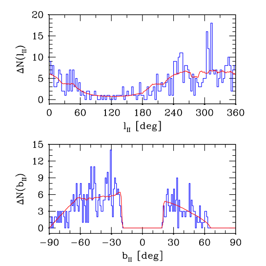
Figure 2: Number of REFLEX clusters of galaxies as a function of galactic longitude $l_{\rm II}$ and latitude $b_{\rm II}$ (steps) compared with the number of clusters expected for a random realisation of the REFLEX selection function (area and sensitivity), computed for the nominal flux limit $3\times 10^{-12}\,{\rm erg}\,{\rm s}^{-1}\,{\rm cm}^{-2}$ and the minimum of 10 source counts (continuous lines). Narrow count bins are chosen to show the effects of large-scale clustering.

The cluster candidates are screened using the X-ray, optical, and literature data. Obvious multiple detections, and candidates with a strong point-like contamination (e.g., active galactic nuclei AGN) of the X-ray flux where the residual flux from the cluster is estimated to be smaller than the nominal REFLEX flux limit, are removed. Double sources are deblended, and count rates measured in the hard band are converted to unabsorbed fluxes in the ROSAT band $(0.1-2.4)$ keV using standard radiation codes for a thermal spectrum with temperature $k_{\rm B}T=5.0$ keV, redshift $z=0$, metal abundance 0.3 solar units, and local $N_{\rm HI}$ (Dickey & Lockman 1990, Stark et al. 1992). The internal errors of the measured fluxes range between 10 and 20 percent. The effects of a possible systematic underestimation of the total fluxes, mainly caused by the incomplete sampling of the outer parts of the cluster X-ray emission, are presently investigated (H. Böhringer et al., in preparation). For the present investigation the measured fluxes (not the total fluxes) are used.

A complete identification of all cluster candidates and a measure of their redshifts has been performed in the framework of an ESO Key Programme (Böhringer et al. 1998, Guzzo et al. 1999). During this campaign, 431 X-ray targets were observed with an average of about 5 spectra per target.

The iterative computation of the X-ray luminosity uses in the first step the redshift and the unabsorbed X-ray flux to give a first estimate of $L_{\rm X}$. This luminosity and the luminosity-temperature relation of Markevitch (1998, without correction for cooling flows) is used to improve the initial temperature estimate ($5$ keV). In the next step the count rate-flux conversion factor is recomputed including now the effects of $z$. The cluster restframe luminosity is calculated by taking into account the equivalent to the cosmic K-correction. The X-ray luminosities are given for the $(0.1-2.4)$ keV energy band ($h=0.5$). For this band and for clusters with redshifts $z\leq 0.3$ and the temperature $T=5$ keV the K-corrections are less than 12 percent. Note that the iterative calculation does not introduce any uncertainty in the selection function, since each value of $L_{\rm X}$ has a unique correspondence to the first calculated unabsorbed flux and thus to a uniquely determined survey volume.

Figure 3: Normalized comoving cluster number densities as a function of redshift, $z$, and comoving radial distance, $R$, computed with $\Omega_{0}=1$. Vertical bars represent the formal $1\sigma$ Poisson errors. Note the quasi-periodic density fluctuations around an essentially constant mean.

Adding to the above mentioned selection criteria the nominal flux limit of the REFLEX sample, $3\times 10^{-12}\,{\rm erg}\,{\rm s}^{-1}\,{\rm cm}^{-2}$ within the ROSAT energy band $(0.1-2.4)$ keV, we find 452 clusters. Of these 449 have measured redshifts, 1 object is clearly a cluster while 2 are unconfirmed candidates. 65 percent of the sample are Abell/ACO/Supplement clusters. However, note the difficulty to compare X-ray flux-limited and richness-limited cluster samples (see Böhringer et al. 2000a for more details). 81 percent of these clusters show a significant X-ray extent (determined with the growth curve analysis method). This shows how a selection based solely on X-ray extent would have missed, given the quality of the RASS II data, a significant percentage of true clusters. Less than 10 percent of the REFLEX sources are expected to be significantly contaminated by unidentified AGN.

Figure 1 shows the spatial distribution of the REFLEX clusters for redshifts $z\leq 0.35$. Galactic extinction partially obscures the regions $6^{\rm h}-10^{\rm h}$ and $16^{\rm h}-20^{\rm h}$. The cone diagrams – although averaged over a large Declination range – illustrate the comparatively high sampling rates obtained with the REFLEX survey. Inhomogeneities in the spatial distribution of clusters on scales of the order of $100\,h^{-1}\,{\rm Mpc}$ are thus easily recognized. A detailed analysis of the behaviour of the mean density and of the topology using Minkowski functionals will be presented in forthcoming papers. However, the combined effect of the X-ray flux-limit and the steep X-ray luminosity function (Böhringer et al., in preparation) introduces a systematic dilution of the sample for larger redshifts. This is an important difference to traditional optical cluster samples which are up to a certain redshift almost volume-limited (for given richness). In the following section the REFLEX data are tested for artifical number density fluctuations which could bias fluctuation measurements on large scales.

3 Tests for artificial density fluctuations

3.1 Variation of the local X-ray flux limit across the survey area (survey sensitivity variations)

The local flux limit is determined by the nominal flux limit, the minimum number of source counts required for a safe detection, the local exposure time in the RASS II, and the local $N_{\rm HI}$ value. According to the resulting survey sensitivity map for $\geq 10$ source counts the nominal flux limit $3\times 10^{-12}\,{\rm erg}\,{\rm s}^{-1}\,{\rm cm}^{-2}$ is reached on 97 percent of the total survey area. For $\geq 30$ source counts the fraction drops to 78 percent. For precise fluctuation measurements it is thus necessary to take into account the local survey sensitivity.

In order to use as many clusters as possible for the fluctuation measurements all sources with at least 10 source counts in the hard band are included. Generally, the comparatively low background of the ROSAT PSPC especially in the hard band allows the detection and the characterization of sources even with low source counts. In fact, the number of clusters with 10 to 29 source counts as observed ($N_{\rm cl}=26$) and as predicted from the subsample of the clusters with at least 30 source counts ($N_{\rm cl}=37$) suggests a formal incompleteness of $11\pm 5$ clusters ($1\sigma$ Poisson error, no cosmic variance) for the subsample with at least 10 source counts. Assuming that the subsample with at least 30 source counts is complete this gives a formal overall incompleteness smaller than 3 percent. The corresponding local incompletenesses are expected to be highest in the areas where the ROSAT satellite passed the radiation belts in the South Atlantic Anomaly of the Earth’s magnetic field.

Random samples are used for the power spectrum analysis giving Monte-Carlo estimates of the actual REFLEX survey windows (Sect. 4). They can also be used to test the quality of the survey selection model. In the following we describe their construction. The sensitivity map is computed for approximately $1^{\circ}\times 1^{\circ}$ tiles covering the complete sky area $\leq 2.5$ deg Declination. Each of the resulting 21 529 local selection functions, $\phi(\@vec{r})$, gives the fraction of the X-ray luminosity function at the comoving distance $\@vec{r}$, and thus the number of expected clusters, $\Delta N(\@vec{r})=\bar{n}\phi(\@vec{r})\Delta V(\@vec{r})$, down to the local flux limit of the given tile, $S_{\rm lim}(\alpha,\delta)$, assuming complete randomness. Here, $\bar{n}$ is the mean comoving cluster number density, $\Delta V(\@vec{r})$ the comoving volume element at $\@vec{r}$, and for the given angular coordinate $(\alpha,\delta)$ of the tile,

$$\phi(\@vec{r})\,=\,\frac{\int_{L_{\rm X}(S_{\rm lim}(\alpha,\delta),z)}^{\infty}\,\Phi(L_{\rm X})\,dL_{\rm X}}{\int_{L_{\rm X}^{\rm min}}^{\infty}\,\Phi(L_{\rm X})\,dL_{\rm X}}\,,$$ (1)

where $L_{\rm X}^{\rm min}$ is the minimum X-ray luminosity of the sample. For the X-ray luminosity function, $\Phi(L_{\rm X})$, we plug in the empirical estimate of the global REFLEX luminosity function as determined in Böhringer et al. (in preparation). The shape of this function can be described by a Schechter function with the characteristic luminosity $L_{*}=6.04\times 10^{44}\,{\rm erg}\,{\rm s}^{-1}$ $(h=0.5)$, and the faint-end slope $\alpha=-1.61$ (for a minimum of 10 source counts, no deconvolution of measurement error, see also de Grandi et al. 1999). The transformation of the cluster restframe luminosities into the observer restframe fluxes corresponds to the reverse of the $S\rightarrow L_{\rm X}$ transformation described in Sect. 2. This prescription gives a good representation of the redshift histogram for $L_{\rm X}^{\rm min}=1.0\times 10^{43}\,{\rm erg}\,{\rm s}^{-1}$ (comparable to the luminosity of bright Hickson groups).

Figure 2 compares the observed cluster surface number densities as a function of galactic coordinates with the surface number densities obtained from Monte-Carlo simulations of a random distribution of clusters in the REFLEX survey area with at least 10 X-ray source counts, and modulated by the local variation of the satellite exposure time and galactic $N_{\rm HI}$ (survey sensitivity map). The overall agreement is encouraging. The good statistical coincidence between observed and expected cluster counts close to the $b_{\rm II}=\pm 20^{\circ}$ survey boundaries suggests that the effects of galactic extinction are well represented in the survey selection model. The remaining local deviations are caused by large-scale clustering.

3.2 Variation of the average comoving cluster number density along the radial direction

To test the variation of the average cluster number density along the radial direction, mean densities are computed for different volume-limited subsamples taking into account the local survey sensitivity map by weighting each cluster with the X-ray flux $S$ using the inverse of the fraction of the survey area with a flux limit below $S$ (effective area). For each subsample the comoving number densities are normalized to their respective mean density.

Figure 3 shows the normalized comoving number density computed along the redshift direction for comoving radial distances of $R\leq 400\,h^{-1}\,{\rm Mpc}$ correspond to $z\leq 0.15$. Maximum fluctuations of the order of 3 are found on small scales. They are successively smoothed out with increasing $R$. The quasi-periodic density variations have a wavelength of about $150\,h^{-1}\,{\rm Mpc}$. No related feature is seen in the power spectrum at this scale (see Sect. 6). The essentially constant mean comoving cluster density implies the absence of selection effects discriminating against the more distant clusters. Note that the REFLEX survey covers the southern hemisphere so that a volume with a radius of $R=400\,h^{-1}\,{\rm Mpc}$ gives a maximum comoving scale length of about $\lambda=2R=800\,h^{-1}\,{\rm Mpc}$. Comoving number densities on Giga parsec scales will be discussed in detail in Böhringer et al. (in preparation).

The huge nearby underdensity centered at $z=0.03$ is also present in the ESO Slice Project data (Vettolani et al. 1997) as shown in Zucca et al. (1997) and might be the origin of the observed deficit of ‘bright’ galaxies in the magnitude number counts as discussed in Guzzo (1997). The large overdensity region at $z=0.05$ is partially caused by the Shapley concentration (Fig. 1 – right cone, see also Scaramella et al. 1989, and Bardelli et al. 1997) and by some isolated nearby structures located at that distance in the direction of the South Galactic Pole (Fig. 1 – left cone).

3.3 Flux-dependent incompletenesses

Flux-dependent incompletenesses might also lead to systematic errors in the fluctuation measurements. This section investigates the presence of this type of incompleteness and its relation to cosmic variance.

 

Figure 4: Cumulative distributions as a function of X-ray flux for a REFLEX subsample (thick continuous line) and for 10 simulated OCDM samples (thin continuous, broken, dotted, dashed lines) convolved with the REFLEX survey sensitivity and normalized to the same number of clusters. The large scatter of the number counts at high fluxes is significantly above the formal Poisson expectation and reflects the effects of cosmic variance.

For the REFLEX flux range the shape of the cumulative cluster number counts as a function of X-ray flux is mainly sensitive to flux-dependent incompleteness and to the K-correction, weakly dependent on evolutionary effects, and almost independent of the shape of a non-evolving X-ray luminosity function (completely independent for an Euclidean space), the chosen cosmological background model, and the type of dark matter used in the simulations. The comparison of the slopes of observed and simulated distributions provides a robust though model-dependent measure of the relative incompleteness of a survey (the N-body simulations are described in Sect. 5.2).

The individual cumulative flux-number counts obtained with 10 statistically independent simulations are shown in Fig. 4. Cosmic variance modulates the simulated cluster counts especially for X-ray fluxes $S>5.0\times 10^{-12}\,{\rm erg}\,{\rm s}^{-1}\,{\rm cm}^{-2}$ yielding slopes between $-1.2$ and $-1.6$. The fluctuations are caused by the large-scale variations of comoving cluster number density at small redshifts similar to those shown in Figs. 1 and 3. At fainter fluxes the fluctuations decrease and the slopes of the cumulative distributions converge to values of about $-1.3$ (note that the plotted cumulative distributions still contain the effects of the effective survey area) which is close to the observed slope of $-1.35$ (Böhringer et al. 2000a). At this limit the REFLEX sample appears to be deep and large enough so that the resulting number counts should be regarded as statistically representative for the local Universe and not dominated by chance fluctuations. The similarity of observed and simulated slopes suggests a high overall completeness of REFLEX.

As a second measure of the overall sample incompleteness the $V/V_{\rm max}$ test (e.g., Schmidt 1968, Avni & Bahcall 1980) is applied as a function of the flux limit. Fig. 5 shows the averaged $V/V_{\rm max}$ values for different X-ray flux limits. Towards fainter flux limits the scatter decreases because sample sizes and volumes increase. At the nominal flux limit, the mean $V/V_{\rm max}$ value is $0.512\pm 0.014$ where the formal error does not include fluctuations caused by large-scale clustering. We take this convergence to the ideal case $<V/V_{\rm max}>=0.5$ for a non-expanding Euclidian universe as a clear sign that at the nominal flux limit the REFLEX survey volume and sample size is large enough to cover a representative part of the local Universe with a high sample completeness and a small sample variance.

Figure 5: Mean $V/V_{\rm max}$ values for REFLEX clusters as a function of X-ray flux. Error bars are the formal $1\sigma$ Poisson errors (no cosmic variance). To illustrate the sensitivity of the test we have computed $V/V_{\rm max}$ also below the nominal flux limit of $3.0\times 10^{-12}\,{\rm erg}\,{\rm s}^{-1}\,{\rm cm}^{-2}$ where no REFLEX clusters are present to mimic a simple kind of incompleteness. Note that the test is performed with all clusters brighter than a given flux limit $S_{(0.1-2.4\,{\rm keV})}$ introducing a statistical dependency of the averaged $V/V_{\rm max}$ values for different $S$.

To summarize, although it is not the basic aim of the present investigation to assess the absolute completeness and statistical representativeness of the REFLEX sample (see Böhringer et al. 2000a), several indications are given that the REFLEX survey is large enough so that in general the values of statistical quantities derived from the sample are expected to be not dominated by the effect of the limited REFLEX survey volume (e.g., Figs. 3,4), and should thus give a useful characterization of the local Universe. The fluctuation measurements investigated here will not be dominated by survey incompleteness (Fig. 5) or other artifical large-scale variations out to radial distances of $400\,h^{-1}\,{\rm Mpc}$ (Fig. 3).

For the following power spectrum analyses we use different subsamples which are either flux-limited (abbreviated by F) or volume-limited (abbreviated by L). Note that the flux limit of the F subsamples is the nominal flux limit of REFLEX and that most of the F subsamples are also restricted to different volumes smaller than the total survey volume (see below). The characteristics of the subsamples are given in Tab. 1. The F0 sample contains all clusters with $L_{\rm X}\geq 10^{43}\,{\rm erg}\,{\rm s}^{-1}$, ($h=0.5$), and source counts $\geq 10$. It serves as a reference sample from which the following subsamples are derived. The subsamples F300 to F800 differ by the chosen box length, $L$, used for the computation of the Fourier transforms, varying between $L=300\,h^{-1}\,{\rm Mpc}$ and $L=800\,h^{-1}\,{\rm Mpc}$. With these subsamples volume-dependent effects are tested. The volume-limited subsamples L050 and L120 have luminosity $L_{\rm X}\geq 0.5\times 10^{44}\,{\rm erg}\,{\rm s}^{-1}$ and $L_{\rm X}\geq 1.2\times 10^{44}\,{\rm erg}\,{\rm s}^{-1}$ ($h=0.5$), respectively, and are used to analyse the amplitude and shape of $P(k)$ for clusters with different masses. For the given flux limit, subsamples with a lower X-ray luminosity cut as used in L050 are surely fluctuation-dominated and can thus not be regarded as statistically representative. L120 has the largest sample size attainable for volume-limited REFLEX subsamples. Tab. 1 gives comoving cluster number densities and mean cluster-cluster distances only for the volume-limited subsamples because of the strong dilution of the flux-limited subsamples and the corresponding large change of these quantities with increasing redshift.

Tab. 1. REFLEX flux-limited (F) and volume-limited (L) subsamples used for the power spectral analyses of the clusters with $\geq 10$ source counts and the nominal flux limit $3.0\times 10^{-12}\,{\rm erg}\,{\rm s}^{-1}\,{\rm cm}^{-2}$, and $L_{\rm X}\geq 10^{43}\,{\rm erg}\,{\rm s}^{-1}$. The X-ray luminositities $L_{\rm X}$ are given for $h=0.5$, box length $L$ used for the Fourier transformation, averaged comoving cluster number densities $n$, and mean cluster-cluster distances, $\bar{s}$, in units of $h$. $N_{\rm CL}$ is the number of clusters in the subsample and $z$ the redshift. Fluxes and luminosities are given for the ROSAT energy band $(0.1-2.4)$ keV.

Sample	$L_{\rm X}\geq$	$z\leq$	$N_{\rm CL}$	$L$	$n$	$\bar{s}$
	$[10^{44}\,{\rm erg}\,{\rm s}^{-1}]$			$[h^{-1}\,{\rm Mpc}]$	$[h^{3}\,{\rm Mpc}^{-3}]$	$[h^{-1}\,{\rm Mpc}]$
F0	$0.1$	$0.460$	$428$	-	-	-
F300	$0.1$	$0.460$	$133$	$300$	-	-
F400	$0.1$	$0.460$	$188$	$400$	-	-
F500	$0.1$	$0.460$	$248$	$500$	-	-
F600	$0.1$	$0.460$	$292$	$600$	-	-
F700	$0.1$	$0.460$	$326$	$700$	-	-
F800	$0.1$	$0.460$	$341$	$800$	-	-
L050	$0.5$	$0.063$	$75$	$400$	$9.0403\times 10^{-6}$	$48.0$
L120	$1.2$	$0.093$	$96$	$400$	$3.8312\times 10^{-6}$	$63.9$

4 Spectral analyses

4.1 Formal background

In the following the spatial distribution of clusters is regarded as a realisation of a formal point process. The corresponding Fourier transforms are well-defined in the strict mathematical sense if the related count measures are approximated by suitably smoothed versions, allowing the application of the classic Bochner-Khinchin theorem (e.g., Shiryaev 1995, p. 287) also for point processes. The subsequent definition of the classical Bartlett or power spectrum of point processes via the Fourier transform of reduced second-order stationary random measures (Ripley 1977), which are closely related to the two-point (spatial) correlation function, does not cause any greater difficulties. More details can be found in, e.g., Daley & Vere-Jones (1988, Chap. 11).

4.2 Spectral estimators

Problems arise to find unbiased spectral estimators with small variance and no correlations between power spectral densities obtained at different wavenumbers $k$. As an example, naive estimators of the general form (statistical estimates are indicated by the hat symbol)

$$\hat{P}(k)\,\sim\,\left|\,\frac{1}{N}\,\sum_{j=1}^{N}\,e^{i\@vec{k}\cdot\@vec{r}_{j}}\,-\,W_{\@vec{k}}\right|^{2}\,,$$ (2)

where $N$ is the number of points which are located at the comoving positions $\@vec{r}_{j}$, and $W_{\@vec{k}}$ the discrete Fourier transform of the survey window, are basically applied in all investigations mentioned in Sect. 1. Even for cubic survey volumes it leads after the subtraction of the shot noise to the expectations (abbreviated by the letter E)

$$\rm{E}\{\hat{\it P}({\it k})\}\,=\,\int\,F(\@vec{k}-\@vec{k}^{\prime})\,P(\@vec{k}^{\prime})\,d^{3}\@vec{k}^{\prime}\,,$$ (3)

where $F(\cdot)$ is known (in the one-dimensional case) as the Fejér’s or Dirichlet’s kernel (Percival & Walten 1993, Chap. 6). The resulting systematic distortions of $\hat{P}(k)$ caused by the sidelobes of $F$ increase with the dynamic range of $P(k)$ and for small data volumes. Tapering is one method to reduce this type of leakage (Blackman & Tukey 1958, p. 93) but would increase the variance of $\hat{P}(k)$ as well. Another method is to estimate the power spectral densities only for those $k$ values where the Fourier transforms of $F(\cdot)$ are almost zero, namely at the multiples of the fundamental mode, $k_{0}=2\pi/L$, where $L$ is the length of the Fourier box. In order to increase the signal-to-noise the power spectral densities are averaged over shells in $k$-space with the thickness $\Delta k=k_{0}$, centered on the multiples of the fundamental mode. In a similar way smoothing of $\hat{P}(k)$ with, e.g., Bartlett, Parzen, or other standard spectral smoothing windows as described in reference books on Fast Fourier transform would reduce the variance of $\hat{P}(k)$. However, as shown in Percival & Walten (1993), either type of smoothing is critical because especially the central lobe of the smoothing window introduces a bias $\sim\gamma^{2}\frac{\partial^{2}P(k)}{\partial k^{2}}$ which is proportional to the squared bandwidth, $\gamma^{2}$ (a reasonable estimate of $\gamma$ is given by the fundamental mode $k_{0}$), and to the local curvature of $P(k)$.

The leakage introduced by the survey window increases even further for asymmetric survey volumes because in this case a unique fundamental mode does not exist. For almost symmetric windows the effects are small and might be corrected using the formulae given in Peacock & Nicholson (1991) and Lin et al. (1996). For highly asymmetric windows the whole concept of plane wave approximation fails. In this case the deconvolution of the survey window function becomes unreliable below a certain wavenumber, and the best solution is to resort to survey- and clustering- specific eigenfunctions as those provided by the Karhunen-Loeve transform (Vogeley & Szalay 1996). Moreover, the survey volume under consideration might not be large enough to cover a representative part of the Universe so that the resulting ‘cosmic variance’ adds to the technical effects described above.

Here, for the determination of the power spectrum, two methods are compared. The first method uses the estimator (Schuecker et al. 1996a,b)

$$\hat{P}(k)\,=\,\frac{V}{\sum_{\@vec{k}^{\prime}}|W_{\@vec{k}^{\prime}}|^{2}}\,\left<\frac{|\hat{\delta}_{\@vec{k}}|^{2}\,-\,\hat{D}}{1-|W_{\@vec{k}}|^{2}}\right>_{|\@vec{k}|}\,,$$ (4)

where the fluctuation amplitudes are corrected for the effects of the survey window by

$$\hat{\delta}_{\@vec{k}}\,=\,\frac{1}{\sum_{i}[\hat{\phi}(\@vec{r}_{i})]^{-1}}\,\sum_{i=1}^{N}\,[\hat{\phi}(\@vec{r}_{i})]^{-1}\,e^{i\@vec{k}\cdot\@vec{r}_{i}}$$

$$\quad\quad\quad\,\,-\,\,\frac{1}{\sum_{j}[\hat{\phi}(\@vec{r}_{j})]^{-1}}\,\sum_{j=1}^{M}\,[\hat{\phi}(\@vec{r}_{j})]^{-1}\,e^{i\@vec{k}\cdot\@vec{r}_{j}}\,.$$ (5)

The estimator of the discreteness noise is

$$\hat{D}\,=\,\frac{\sum_{i=1}^{N}(\hat{\phi}(\@vec{r}_{i}))^{-2}}{\left[\sum_{i=1}^{N}(\hat{\phi}(\@vec{r}_{i}))^{-1}\right]^{2}}\,+\,\frac{\sum_{j=1}^{M}(\hat{\phi}(\@vec{r}_{j}))^{-2}}{\left[\sum_{j=1}^{M}(\hat{\phi}(\@vec{r}_{j}))^{-1}\right]^{2}}\,.$$ (6)

The squared differences of the discrete Fourier transforms of the observed (inhomogeneous) and of the random distributions, both corrected for shot noise, are averaged over different directions and weighted by $(1-|W_{\@vec{k}}|^{2})$ reducing the effects of the errors in the mean number density (Peacock & Nicholson 1991). The power spectral densities must be normalized by the volume $V$ used to compute the Fourier transforms and by the total power of the Fourier transformed survey window. Whereas the number of observed objects $N$ is fixed by the sample, the number of points used for the random sample $M$ should be large enough so that their shot noise contributions can be subtracted with high accuracy. Both the observed and the random samples have the same position-dependent selection function, $\phi(\@vec{r})$.

The second method to determine the power spectrum averages the fluctuation power over $N_{k}$ modes per $k$ shell (Feldman, Kaiser & Peacock 1994),

$$\hat{P}(k)=\frac{1}{N_{k}}\,\sum_{\@vec{k}}|\hat{\cal{F}}(\@vec{k})|^{2}-\hat{\cal{D}}\,,$$ (7)

where the window-corrected Fourier-transformed density contrasts are given in a similar way as before,

$$\hat{\cal{F}}(\@vec{k})\,=\,\sum_{i=1}^{N}\,w(\@vec{r}_{i})\,e^{i\@vec{k}\cdot\@vec{r}_{i}}\,-\,\alpha\,\sum_{j=1}^{M}\,w(\@vec{r}_{j})\,e^{i\@vec{k}\cdot\@vec{r}_{j}}\,.$$ (8)

The total shot noise is estimated by

$$\hat{\cal{D}}\,=\,\alpha(1+\alpha)\,\sum_{j=1}^{M}w^{2}(\@vec{r}_{j})\,e^{-\@vec{k}\cdot\@vec{r}_{j}}\,,$$ (9)

where $\alpha=N/M$. For Gaussian fluctuations the weights $w(\@vec{r})\,=\,\frac{1}{1\,+\,n(\@vec{r})\,P(k)}$ minimize the variance of the estimator, however, they require the a priori knowledge of $P(k)$, that is, the quantity one wants to measure, in addition to a fair estimate of the mean density, $n(\@vec{r})$. Reasonable results are attainable if $n(\@vec{r})$ is estimated by the observed luminosity function or by smoothed empirical $z$ histograms (Sect. 3.1) and the sensitivity map of the survey, and if $P(k)$ is approximated by a constant power spectrum, $P(k)=P_{0}={\rm const}$.

5 Test of the spectral analyses

5.1 General tests

Figure 6: Power spectral densities obtained with eq. 4 (‘standard method’ STD) and with eq. 7 (‘Feldman, Kaiser, Peacock method’ FKP) for a flux-limited REFLEX subsample with $N=188$ clusters within a cubic volume $V=(400\,h^{-1}\,{\rm Mpc})^{3}$. The radial parts of the random samples used to estimate the survey window are computed with smoothed empirical $z$ histograms.

The first test concerns the choice of the spectral estimator used for the analyses of the REFLEX data. Fig. 6 compares the estimates obtained with eqs. (4) and (7). The power spectral densities are computed for a flux-limited REFLEX subsample in a cubic box with a length of $L=400\,h^{-1}\,{\rm Mpc}$ using a standard FFT algorithm on a $128^{3}$ grid for $N=188$ REFLEX clusters and for $M=2.0\times 10^{6}$ random particles. The differences between the power spectral densities obtained with eqs. (4) and (7) and the differences between the power spectra obtained with (7) for different $P_{0}$ are small compared to the errors introduced by the sample itself (see Sect. 5.2). We choose (4) for the spectral analyses because the exploration of the REFLEX data should start with a minimum of pre-assumptions about $P(k)$. Moreover, the REFLEX survey volume is comparatively symmetric so that in addition to the window correction term in eq. (4) no specific deconvolutions are performed. The remaining effects of the window functions are checked using the results obtained with N-body simulations (see Sect. 5.2).

Figure 7: Fluctuation power spectral densities, $P(k)$, as a function of comoving wavenumber, $k$, corresponding to the wavelength $\lambda=2\pi/k$. Compared are REFLEX $P(k)$ obtained with two different methods to compute the radial part of the reference random sample. Filled symbols are obtained with random samples based on the X-ray luminosity function (XLF), open symbols are based on smoothed redshift histograms of observed samples (SMOOTH).

To test the robustness of the method applied for the computation of the radial parts of the random samples (see Sect. 3.1) the empirical $z$ histogram is determined for different flux limits and smoothed with the biweight kernel (corrected for edge effects) using the standard deviation $\sigma_{z}=0.03$ to reduce the large-scale fluctuations. The filtered redshift distributions give an alternative representation of the radial selection functions (after proper normalization with the comoving volume elements and the survey sensitivity map). The local redshift distribution of the random sample as well as the local radial selection function is then estimated by the Monte-Carlo method.

Figure 8: REFLEX (continuous) and simulated (dashed-dotted) cluster redshift histograms.

                          

Figure 9: Power spectra for simulated (OCDM) flux-limited subsamples in different volumes. Filled symbols give the average power spectral densities obtained by imposing the REFLEX survey conditions, continuous lines the average power spectral densities obtained for all-sky cluster surveys with uniform survey sensitivities and no galactic extinction, but with the same X-ray luminosity function as the corresponding REFLEX subsamples (error bars omitted). The error bars are the $1\sigma$ standard deviations of the power spectral densities obtained with 10 REFLEX-like simulations. Error bars exceeding the plotted $P(k)$ range are shown by arrows. The size of the Fourier box and the average number of simulated clusters located in the box is given in the lower left of each panel.

As an example, the power spectral densities shown as open symbols in Fig. 7 are computed with random samples based on smoothed empirical $z$ distributions, the filled symbols with random samples based on the REFLEX X-ray luminosity function. It is seen that the power spectral densities obtained with the smoothing method are systematically smaller up to factors reaching 1.6 at the largest scales. The differences at small scales are mainly caused by the poor sampling of density waves by the REFLEX clusters. We regard the luminosity function method to be more reliable, especially on large scales (and for small sample sizes): smoothing out all fluctuations is almost impossible, especially on large scales, so that the resulting spectra have systematically smaller amplitudes as illustrated by Fig. 7. In the following all REFLEX power spectra excluding those shown in Fig. 6 are obtained by using the luminosity function to compute the radial part of the random samples.

Tab. 2: REFLEX power spectral densities obtained for different REFLEX subsamples, indicated by the index (see Tab. 1) of the power spectral densities, $P$. The errors are the formal $1\sigma$ standard deviations as adapted from 10 OCDM simulations.

$$\hskip 14.22636pt\begin{array}[]{|rrr|rrr|rrr|r|rr|rr|}\hline\cr\vskip 3.0pt plus 1.0pt minus 1.0pt\cr k&P_{\rm F300}(k)&\sigma(P)&k&P_{\rm F400}(k)&\sigma(P)&k&P_{\rm F500}(k)&\sigma(P)&k&P_{\rm L050}(k)&\sigma(P)&P_{\rm L120}(k)&\sigma(P)\\ \vskip 3.0pt plus 1.0pt minus 1.0pt\cr\hline\cr 0.0209&225005&165087&0.0157&75312&65600&0.0126&573540&301495&0.0157&208388&122391&392794&301752\\ 0.0419&295582&166814&0.0314&203050&119346&0.0251&261792&114413&0.0314&283215&203881&453834&346729\\ 0.0628&130385&73346&0.0471&180709&100744&0.0377&355915&274882&0.0471&423245&227117&482384&366700\\ 0.0838&75460&24608&0.0628&143612&75696&0.0503&156029&59838&0.0628&218190&82455&428681&230770\\ 0.1047&71151&26249&0.0785&96808&57489&0.0628&50935&23333&0.0785&187649&97309&355547&293808\\ 0.1257&54969&27508&0.0942&75444&41117&0.0754&123809&80121&0.0942&105025&68010&281954&268664\\ 0.1466&54289&31769&0.1100&83073&30014&0.0880&82749&40760&0.1100&101841&65454&223302&172965\\ 0.1676&47469&12606&0.1257&31639&8920&0.1005&82533&18233&0.1257&70705&30683&131183&95468\\ 0.1885&34690&24804&0.1414&39688&21014&0.1131&48720&20268&0.1414&63820&36793&100848&62951\\ 0.2094&33145&24350&0.1571&40994&20666&0.1257&35619&17539&0.1571&51805&30448&121818&90020\\ 0.2304&33044&19821&0.1728&34105&13942&0.1382&68543&23563&0.1728&62935&60617&110103&60398\\ 0.2513&23607&16395&0.1885&22950&15291&0.1508&45761&19363&0.1885&51164&34999&93618&77630\\ 0.2723&15823&13983&0.2042&24635&8116&0.1634&30936&14519&0.2042&47937&25678&70140&28187\\ 0.2932&16462&12553&0.2199&19413&8452&0.1759&48897&32916&0.2199&55192&41352&84617&38806\\ 0.3142&19420&11962&0.2356&21710&12222&0.1885&20998&7960&0.2356&48857&33925&81083&70289\\ 0.3351&19051&16859&0.2513&21041&11528&0.2011&26694&11482&0.2513&41602&20935&75968&79354\\ 0.3560&6133&2189&0.2670&6694&5141&0.2136&10775&2504&0.2670&38002&21234&65442&51403\\ 0.3770&11933&13125&0.2827&10279&8592&0.2262&7637&4614&0.2827&42094&28279&81393&68258\\ 0.3979&7290&3426&0.2985&15554&11277&0.2388&10707&6913&0.2985&36277&17070&70096&53046\\ &&&0.3142&10472&7294&0.2513&10938&5870&0.3142&35870&19565&61827&60854\\ &&&&&&0.2639&9894&5652&0.3300&33286&17785&49837&18589\\ &&&&&&0.2765&10248&8046&0.3456&20573&16773&32071&40253\\ &&&&&&0.2890&8869&4518&0.3613&21151&15062&34525&25173\\ &&&&&&0.3267&8259&4428&0.3770&19253&19786&43460&30951\\ &&&&&&&&&0.3927&20295&20823&29257&21929\\ \vskip 3.0pt plus 1.0pt minus 1.0pt\cr\hline\cr\end{array}$$

5.2 N-body simulations

Systematic and random errors of $\hat{P}(k)$ are investigated using a set of statistically independent cluster distributions obtained from realistic N-body simulations, transformed into redshift space, and modified according to the REFLEX survey selection as summarized by the survey sensitivity map. In the following a brief overview of some technical aspects of the simulations are given. A more detailed description will be presented in the second paper on the REFLEX power spectrum.

The simulations are performed using a standard PM code (Hockney & Eastwood 1988) with $256^{3}$ particles in a $(500\,h^{-1}\,{\rm Mpc})^{3}$ box on a $512^{3}$ grid giving the force resolution $\Delta x\approx 1\,h^{-1}\,{\rm Mpc}$. Ten OCDM models are simulated with the parameters $h=0.60$, cosmic density parameter of matter, $\Omega_{0}=0.40$, cosmological constant $\Omega_{\Lambda}=0$, cosmic density parameter of baryons, $\Omega_{\rm b}=0.05$ (this corresponds to an estimate of Burbles & Tytler 1998) and $\sigma_{8}=0.80$. The transfer function was calculated with the Boltzmann code CMBFAST of Seljak & Zaldamiaga (1996). The normalization is so as to provide the correct cluster abundance satisfying both the relation given in Eke, Cole & Frenk (1996) and in Viana & Liddle (1996). We chose this model because it gives a good representation of the REFLEX data and thus realistic error estimates. However, any other model with a similar power spectrum could do the job as well. The mass resolution is $8.4\times 10^{11}\,h^{-1}\,M_{\odot}$. Each simulation starts at the redshift $z=50$ (initial perturbations imposed on the ‘glass-like’ initial load using the Zel’dovich approximation) and ends after 245 time steps (increment of the scale factor $\Delta a=0.004$). Several replicants of the same simulation are combined using periodic boundary conditions to compare results on larger scales. However, only for scales $\leq 500\,h^{-1}\,{\rm Mpc}$ statistically independent measurements can be obtained.

For the identification of the clusters the friend-of-friend method (Davis et al. 1985) is used with the linking parameter $b=0.16$ to pick up virialized structures. The total cluster masses are computed within the radius where the average density ratio is $\bar{\rho}(r_{500})/\rho_{\rm critical}=500$ using only those clusters with at least 10 particles. The masses are transformed into luminosities with the empirical mass – X-ray luminosity relation for $r_{500}$ from (Reiprich & Böhringer 1999),

$$\frac{M}{h^{-1}\,{\rm M_{\odot}}}\,=\,2.52\times 10^{14}\,\left(\frac{L_{\rm x}}{10^{44}\,h^{-2}\,{\rm erg}\,{\rm s}^{-1}}\right)^{0.81}\,.$$ (10)

The individual cluster masses used to derive (10) show a $1\sigma$ scatter of about 50 percent. The $r_{500}$ radius and the OCDM model parameters mentioned above lead to realistic spatial cluster distributions, especially redshift histograms (Fig. 8) and sample sizes, and thus to realistic error estimates for $\hat{P}(k)$. Whereas in the present investigation the model parameters taken from the literature are not changed, studies are in preparation using the ‘standard’ radius $r_{200}$ (see Sect. 7.1) and different types of structure formation models to adjust the parameter values in order to reconcile the models with the observations. We apply the above equation assuming no intrinsic scatter of the mass-luminosity relation. A simulated cluster is rejected if its flux is below the local flux limit given by the survey sensitivity map (for 10 source counts). In this way the simulated cluster sample follows the same sensitivity pattern as the observed REFLEX sample. Finally, sample sizes are adjusted using the additional lower luminosity limit $L_{\rm X}=3\times 10^{43}\,{\rm erg}\,{\rm s}^{-1}$ ($h=0.5$), corresponding to a minimum of 46 particles per cluster. This approximate modeling gives realistic spatial cluster distributions and is enough for the error estimation of $\hat{P}(k)$.

As a brief overview, Fig. 8 illustrate the similarity of the observed and simulated cluster samples (see also the cumulative flux-number counts in Fig. 4). The model parameters are not yet fully optimized to fit the observed data in detail. A more quantitative comparison is given in Sect. 7.

Figure 9 shows the power spectra obtained from (a) simulated data under realistic REFLEX survey conditions (filled symbols), and (b) simulated all-sky cluster surveys with uniform survey sensitivities and no obscuration due to galactic extinction (continuous lines). The error bars of the latter measurements are omitted. The X-ray luminosity functions of the two sets of simulations are identical so that it is straightforward to test whether the power spectral estimator gives the correct power spectrum: after the correct elimination of the effects of the REFLEX survey window (see eq. 4.2) the resulting power spectra (shape and amplitude) of realistic and all-sky simulations should be the same. The simulations correspond to the F300 to F500 REFLEX subsamples (Tab. 1). The errors shown in Fig. 9 represent the $1\sigma$ standard deviations obtained from a set of 10 different OCDM realizations. For these simulations a maximum of $\hat{P}(k)$ is expected at $k\approx 0.02\,h\,{\rm Mpc}^{-1}$. Note that the shape and amplitude of the ideal power spectrum can be recovered under REFLEX conditions in all volumes analyzed. Some extra power is seen at the fundamental mode in the $400$ and $500\,h^{-1}\,{\rm Mpc}$ results, however within the $1\sigma$ range. Note that the $(500\,h^{-1}\,{\rm Mpc})^{3}$ simulations do not give a good representation of the fundamental mode at $k=2\pi/500\,h\,{\rm Mpc}^{-1}$ – only 3 modes are realized per simulation – and do not include any fluctuations on larger scales, so that one should take the error bars obtained at the simulation limit with caution. Nevertheless, the overall agreement of the power spectra obtained under REFLEX and ideal survey conditions suggests that no significant systematic errors of $\hat{P}(k)$ are expected.

6 Observed power spectra

6.1 Exploring the general shape of $\hat{P}(k)$

Figure 10: REFLEX power spectra of the flux-limited subsamples F300 to F500 (filled symbols, monitored by the N-body simulations) and F600 to F800 (open symbols) in volumes with box lengths between $300$ and $800\,h^{-1}\,{\rm Mpc}$ (no corrections for differences in effective biasing). For reference, the spectral fits obtained with the phenomenological model (continuous line) and with the CDM-like model (dashed line) using the subsamples F300 to F800 are superposed.

Many variants of cosmic structure formation models discussed today predict an almost linear slope of the power spectrum on scales $<40\,h^{-1}\,{\rm Mpc}$ and a turnover into the primordial regime between $100$ and $300\,h^{-1}\,{\rm Mpc}$. To summarize our measurements in this interesting scale range, Fig. 10 shows the power spectral densities obtained with the flux-limited REFLEX subsamples F300 to F800. The volumes differ by a factor 19, enabling tests of possible volume-dependent effects (Sect. 6.2). The superposed continuous and dashed lines in this and the following figures of this section are always the same. Their computation and interpretation is described in Sect. 6.2. In the following they may serve as a mere reference to compare the power spectra obtained with the different REFLEX subsamples listed in Tab. 1. Fig. 11 gives a more detailed view of the spectra obtained with the subsamples F300 to F500 in volumes which are monitored by our N-body simulations. Fig. 12 compares the spectra obtained for the volume-limited subsamples L050 and L120 with the spectrum obtained for the flux-limited subsample F400, all spectra are estimated within the same Fourier volume. Finally, Fig. 13 shows the combined power spectrum obtained with the subsamples F300 to F500 which we regard as the basic result of the REFLEX power spectrum analyses. The values of the power spectral densities obtained with the subsamples F300-F500, L050, and L120 with the errors estimated with the N-body simulations are given in Tab. 2. In the following a few more detailed remarks are given.

                          

Figure 11: REFLEX power spectra of the flux-limited subsamples F300 to F500. The box lengths and the number of clusters used for the power spectrum estimation are given in each panel in the lower left. The bars represent the $1\sigma$ errors adapted from N-body simulations. The fits of a linear power spectrum model (dashed lines) and of the phenomenological model (continuous line) using the subsamples F300 to F800 are superposed.

                          

Figure 12: REFLEX power spectra of the volume-limited subsamples L120 (upper panel), and L050 (middle panel), and of the flux-limited subsample F400 (lower panel). L120 contains clusters with a brighter lower X-ray luminosity compared to L050 (and F400). The bars represent the $1\sigma$ errors adapted from N-body simulations. For reference the fits obtained with the phenomenological model (continuous lines) and with the CDM-like model (dashed lines) using the subsamples F300 to F800 are superposed. The amplitudes of $P(k)$ increase with increasing lower luminosity limit as expected by standard biasing schemes.

Figure 10 shows the superposition of the power spectra obtained with the flux-limited subsamples F300 to F800 in the comoving volumes ranging from $(300\,h^{-1}\,{\rm Mpc})^{3}$ to $(800\,h^{-1}\,{\rm Mpc})^{3}$. The data are not corrected for sample-to-sample variations of the effective biasing (see Sect. 7) so that the effective variance among the estimates is possibly smaller than that displayed by the figure. The point distribution outlines a corridor which can be separated into three parts. For $k>0.1\,h\,{\rm Mpc}^{-1}$ the power spectral densities decrease approximately as $k^{-2}$. Between $0.02\leq k\leq 0.1\,h\,{\rm Mpc}^{-1}$ the spectra bend into a flat distribution. The N-body simulations give $1\sigma$ standard deviations between 30 and 80 percent (including cosmic variance) in this scale range as shown in Figs. 11, 12, 13. For $k<0.02\,h\,{\rm Mpc}^{-1}$ a second maximum is seen at $k\approx 0.01\,h\,{\rm Mpc}^{-1}$. We did not perform N-body simulations for such large scales. However, the delete-d jackknife resampling method (a variant of the boostrap method where the creation of artifical point pairs is avoided; see, e.g., Efron & Tibshirani 1993, see also the critical remarks on the use of the bootstrap method in point process statistics given in Snethlage 2000) gives $1\sigma$ error estimates of the order of 80 percent (cosmic variance not included). The detection of the second maximum in the power spectrum on such large scales, if real, would have very important implications on current structure formation models. However, as pointed out in the Introduction, measurements on such large scales are easily biased by very small systematic errors of the survey detection model. We postpone a detailed study of this very questionable feature to a subsequent paper. The present investigation concentrates more conservatively on the range $0.013\leq k\leq 0.4\,h\,{\rm Mpc}^{-1}$ which is found to be free from any significant artifical fluctuations (Sect. 3), which can be easily monitored by the available N-body simulations, and which contains density waves well sampled by the REFLEX clusters.

Figure 13: Combined REFLEX power spectrum obtained with the flux-limited subsamples F300 (open squares), F400 (filled hexagons), F500 (open hexagons), and their standard $1\sigma$ deviations adapted from N-body simulations. Not shown are the power spectral densities with wavenumbers $k\geq 0.4\,h\,{\rm Mpc}^{-1}$ because the corresponding density waves are only sparsely sampled by REFLEX. The continuous line is a fit of the phenomenological model, the dashed line the CDM-like model fit using the flux-limited subsamples F300 to F800. The power spectral density at $500\,h^{-1}\,{\rm Mpc}$ is part of the extra power detected at $k\approx 0.01\,h\,{\rm Mpc}^{-1}$ and might already be biased.

Individual spectra obtained with the three flux-limited subsamples F300 to F500 are shown in Fig. 11, now including the $1\sigma$ errors adapted from the N-body simulations. Whereas the spectra obtained with F300 and F400 (upper and middle panel) show a maximum at $k\approx 0.03\,h\,{\rm Mpc}^{-1}$, the F500 data (lower panel) suggest only a flattening of the spectral densities. Especially the power spectral density obtained at the fundamental mode seems to indicate a still rising power spectrum for smaller $k$ values. A similar effect is seen in the simulations (see Fig. 9) suggesting a statistically not very significant but noticable leakage of fluctuation power especially from the second to the first fundamental mode. The reference to Fig. 10 reveals that the fundamental mode of F500 is already part of the second probably not real maximum in the power spectrum at $k\approx 0.01\,h\,{\rm Mpc}^{-1}$. Hence the fundamental mode of F500 should not necessarily get the highest weight in the evaluation of the maximum of the power spectrum on smaller scales. We test the possibility that the location of the maximum increases with volume but could not find any systematic effect (see Sect. 6.2).

The spectra shown in Fig. 12 obtained with the volume-limited subsamples L050 and L120 (upper and middle panel) show a broad maximum at $k\approx 0.03\,h\,{\rm Mpc}^{-1}$. A weak indication is found for a positive slope on larger scales. The second maximum of the power spectrum seen in Fig. 10 is not sampled by L050 and L120 because their sample volumes do not reach such large scales. The Fourier volumes are therefore restricted in both cases to $(400\,h\,{\rm Mpc}^{-1})^{3}$. For comparison the lower panel shows the power spectrum obtained with the flux-limited subsample F400 estimated within the same volume as used for L050 and L120. In general, the overall shapes of the spectra obtained with the volume- and flux-limited subsamples are found to be similar, although minor differences might be seen on smaller scales (see below). The three spectra also show that the amplitude increases with increasing lower X-ray luminosity of the subsample. However, larger sample sizes are needed to confirm the effect.

To summarize, basically all REFLEX spectra are consistent with a broad maximum of the cluster power spectrum at comoving wavenumbers around $k\approx 0.03\,h\,{\rm Mpc}^{-1}$ corresponding to wavelengths of about $200\,h^{-1}\,{\rm Mpc}$. A second maximum is found at $k=0.01\,h^{-1}\,{\rm Mpc}$ corresponding to $600\,h^{-1}\,{\rm Mpc}$, but appears questionable (see Sect. 8). These findings are summarized in Fig. 13, showing the combined spectra obtained with the subsamples F300 to F500, and illustrating the stability of the results obtained within different volumes. We regard this as a representative REFLEX power spectrum.

6.2 First cosmological implications

In the following we want to characterize the overall shape of the observed power spectra as well as specific spectral features like the location of the maximum and the local slope of $P(k)$ in specific $k$ ranges, restricting the discussion mainly to the conservative $k$ range $0.013\leq k\leq 0.4\,h\,{\rm Mpc}^{-1}$ mentioned above. This will enable us to derive our first cosmological implications.

The REFLEX power spectral densities shown in the last sections are sampled strictly following the rules of standard Fourier analysis. As a consequence we have to work with uncomfortably large but statistically almost independent $k$ bins which complicates the analyses even of the maximum of $\hat{P}(k)$ in the conservative $k$ range. To improve the ‘eye ball’ estimates of the location of the maximum of the power spectra given in Sect. 6.1 and to get a handle of the expected errors, the spectra are parameterized in two different ways. The first method applies a purely phenomenological fitting function which gives an almost model-independent description of the data (see also Peacock 1999, p. 530):

$$P(k)=A\,k_{0}^{-i_{1}}\,k^{i_{1}-3}\,\left[1+\left(\frac{k_{\rm c}}{k}\right)^{i_{2}}\right]^{-1}\,.$$ (11)

The location of the maximum of the power spectrum is

$$k_{\rm max}=k_{\rm c}\left(\frac{-n}{n_{\rm s}}\right)^{\frac{1}{n-n_{\rm s}}}\,.$$ (12)

The slope on large scales, $n=i_{1}+i_{2}-3$, is set to ‘1’ because no statistically reliable information is attainable from the REFLEX data in this scale range. The slope on small scales is $n_{\rm s}=i_{1}-3$. The characteristic scale, $k_{\rm max}$, is comparable to the wavenumber corresponding to the horizon length at the epoch of matter-radiation equality, $k_{\rm eq}=0.195\,\Omega_{0}\,h^{2}\,{\rm Mpc}^{-1}$ (see Peebles 1993, p. 164, and Peacock 1999, p. 459), and thus yields an estimate of the cosmic mass density (assuming that 3 relativistic neutrino families are left over from high redshift, and that neutrino masses are small compared to the temperature of the cosmic microwave background radiation),

$$\Omega_{0}\,h\,=\,5.13\,\frac{k_{\rm max}}{h\,{\rm Mpc}^{-1}}\,.$$ (13)

In contrast to the first method which allows a variable slope at small scales and a narrow maximum, the second method is less flexible, but physically better defined. The fitting function is based on the CDM linear transfer function, $T(k)$, as given in Bardeen et al. (1986), where the power spectrum, $P(k)=AkT^{2}(k)$, again is assumed to have $n=1$ on very large scales. The shape of the power spectrum is characterized by the shape parameter, $\Gamma$, defined in the standard way (eq. 19), giving the approximate relation between $\Gamma$ and $k_{\rm max}$

$$k_{\rm max}\,=\,0.114\,\Gamma\,h\,{\rm Mpc}^{-1}\,.$$ (14)

For CDM-like models with low baryon density, $\Gamma$ is mainly determined by $\Omega_{0}$, $h$, and $\Omega_{\rm b}$ (see eq. 19). This equation offers another way to approximate the cosmic mass density via

$$\Omega_{0}\,h\,\approx\,\Gamma.$$ (15)

A standard SIMPLEX $\chi^{2}$ minimization method is applied separately to the spectra obtained with the subsamples F300 to F800 to perform numerical fits from which the values of $k_{\rm max}$ and $\Gamma$ are deduced. This assumes that the power spectral densities of each individual spectrum are statistically independent. For the given REFLEX survey window ($|W_{k}|^{2}\leq 0.082$ for all $k$ and volumes studied), and for the given spacing of the $k$ values of the measured $P(k)$ data at the multiples of the fundamental mode this is approximately the case. The values of $k_{\rm max}$ and $\Gamma$ obtained from the fits are independent of the volumes used to perform the Fourier analyses as shown in Fig. 14, strongly supporting the detection of a real maximum of $P(k)$ in the given $k$ range. Averages and their formal $1\sigma$ standard deviations of $k_{\rm max}$ and $\Gamma$ using the subsamples F300 to F800 give for the two fit functions, respectively,

                        

Figure 14: Upper panel: values of the shape parameter, $\Gamma$, as a function of the box length, $L$, of the Fourier volume, obtained from fits of the linear CDM model to the flux limited subsamples F300 to F800 (from left to right). Lower panel: values of the wavenumber of the maximum of the power spectrum, $k_{\rm max}$, as a function of $L$ obtained from fits of the phenomenological model. The sample averages are indicated by dashed lines.

$$k_{\rm max}\,=\,0.030\pm 0.005\,,\quad\quad\Gamma\,=\,0.195\pm 0.055\,.$$ (16)

The $\Gamma$ estimate corresponds to $k_{\rm max}=0.022\pm 0.006$. Similar numbers are obtained when only the subsamples F300 to F500 are used. Note that the subsamples F300 to F800 are statistically dependent so that the error estimates given in (16) must be regarded as lower limits. The phenomenological and the CDM-like model based on these mean values are shown as continuous and dashed lines, respectively, in the Figs. 10, 11, 12, 13, and 16. They both give a good description of the shape of all power spectra obtained with the flux- and with the volume-limited REFLEX subsamples. In Fig. 13 we show this for the combined power spectrum obtained with the flux-limited subsamples F300 to F500. The two methods give consistent results for the location of the maximum of the REFLEX power spectra in the range

$$0.022\pm 0.006\,\leq\,k_{\rm max}\,\leq\,0.030\pm 0.005\,h\,{\rm Mpc}^{-1}\,.$$ (17)

Similarily, the values of the cosmic density parameter obtained with eq. (13) and $k_{\rm max}$ from (16), and with eq. (15) and $\Gamma$ from (16) give the range

$$0.15\pm 0.03\,\leq\,\Omega_{0}\,h\,\leq\,0.20\pm 0.06\,.$$ (18)

It is interesting to note that the spectral slopes on small scales of the volume-limited subsamples L050 and L120 estimated by fitting (11) are found to be slightly flatter, $n_{\rm s}=-1.6\pm 0.4$, compared to $n_{\rm s}=-1.8\pm 0.4$ obtained with the flux-limited subsamples ($1\sigma$ error estimates from N-body simulations). However, the differences are statistically perhaps not very significant and might be attributed to cosmic variance.

Figure 15: Combined REFLEX power spectrum obtained with the subsamples F300 to F500 (filled symbols) compared to the power spectrum obtained from Abell/ACO clusters (open hexagons) by Retzlaff et al. (1998) and from APM clusters (open squares) by Tadros et al. (1998).

Figure 16: Combined power spectrum obtained with the REFLEX cluster subsamples F300 to F500 (filled symbols, measurements on scales $<20\,h^{-1}\,{\rm Mpc}$ omitted) compared with the power spectrum of Durham/UKST galaxies (open symbols) obtained by Hoyle et al. (1999). The upper lines give the fit to the REFLEX cluster power spectra, the lower lines the same fits divided by the squared ‘biasing factor’ $b^{2}=2.6^{2}$. The continuous line is a fit of the phenomenological model (Par), the dashed line the CDM-like model fit (CDM) as described in Fig. 13.

Figure 15 compares the REFLEX power spectrum with the Abell/ACO (Retzlaff et al. 1998, see also Einasto et al. 1997) and the APM (Tadros et al. 1998) spectra. The respective amplitudes of the power spectra of the Abell/ACO and APM samples are 1.7 and 2.2 below REFLEX. This might be attributed to the different cluster luminosities contained in the samples. For $k\geq 0.08\,h\,{\rm Mpc}^{-1}$ the spectra give consistent slopes of approximately $-1.8$ although both the REFLEX and the Abell/ACO sample do not show the minimum at $k\approx 0.1\,h\,{\rm Mpc}^{-1}$ found with the APM sample. Regarding the maximum of $P(k)$ the Abell/ACO data suggest a comparatively narrow peak at $k_{\rm max}=0.05\,h\,{\rm Mpc}^{-1}$ consistent with the estimate of Einasto et al. (1997). Contrary to this the REFLEX spectrum has a broad maximum which peaks in the range $0.022\leq k_{\rm max}\leq 0.030\,h\,{\rm Mpc}^{-1}$. Note that the exact evaluation of the statistical significance of this difference is difficult to assess because the REFLEX and Abell/ACO power spectra are sampled in different ways. The broad maximum of the REFLEX spectrum appears to be more consistent with the APM sample if the REFLEX measurement at $500\,h^{-1}\,{\rm Mpc}$ is excluded.

Figure 16 compares the combined REFLEX power spectrum obtained with the flux-limited subsamples F300 to F500 with the spectrum obtained with a magnitude-limited sample of Durham/UKST galaxies (Hoyle et al. 1999). We chose this sample because of the comparatively large samples size (2501 galaxies, 1 in 3 sampling rate), the large volume (1 450 square degrees, $z\leq 0.1$), and the small effects of the survey window. Recall that the upper continuous line is the fit of the phenomenological model to the REFLEX data, the upper dashed line the fit of the CDM-like model; the lower lines are the same fits shifted by the factor $6.8$. For wavelengths $20<\lambda<300\,h^{-1}\,{\rm Mpc}$ the overall shapes of the cluster and galaxy power spectra are very similar. The ratio of the linear biasing factors for the given REFLEX cluster subsample and the galaxy sample as deduced from the shift factor is $b=2.6$.

7 Comparison with CDM models

7.1 Semi-analytic model

To make a first comparison with cosmological models and an attempt to differentiate between their presently discussed variants, an outline of a semi-analytic model is given for biased nonlinear power spectra in redshift space for clusters of galaxies. The model gives a good overview of the effects of different model parameters and is used to narrow the parameter ranges needed for a more detailed comparison with N-body simulations. Notice that a significant number of N-body simulations has to be performed for each parameter set in order to derive statistical meaningful error estimates which is planned for the second paper on the REFLEX power spectrum. The model spectra are computed with parameter values taken from the literature and are compared with the REFLEX power spectra. No evolution of structures is assumed within the redshift range covered by the REFLEX subsamples analyzed ($z<0.15$, for an exact treatment see also Magira et al. 2000). The linear power spectrum $P(k)\sim k^{n}\,T^{2}(k)$ is normalized by the standard deviation of the density contrast, $\sigma_{8}$, obtained with the spherical top hat filter function with the filter radius $R=8\,h^{-1}\,{\rm Mpc}$. The fitting formula for the linear transfer function, $T(k)$, from Bardeen et al. (1986) is applied with the shape parameter (Sugiyama 1995)

$$\Gamma\,=\,\Omega_{0}\,h\,\exp\left(-\Omega_{\rm b}-\sqrt{\frac{h}{0.5}}\frac{\Omega_{\rm b}}{\Omega_{0}}\right)\,,$$ (19)

appropriate for models with low present baryon densities, $\Omega_{\rm b}$. The mapping between evolved and non-evolved real-space power spectra can be deduced from fits to the results obtained with N-body simulations (Hamilton et al. 1991, Peacock & Dodds 1994). We apply the prescription in the form presented in Mo, Jing & Börner (1997, and references given therein). The approximation of the linear growth factor at redshift zero is taken from Carroll, Press & Turner (1992). It was shown that this mapping is almost independent of the slope of the linear power spectrum. Moreover, as long as the strongly non-linear clustering regime is excluded the formalism reproduces the power spectra obtained from N-body simulations quite well.

To compute the observed or effective biasing values Moscardini et al. (2000, see also Matarrese et al. 1997 and Borgani et al. 1999) assumed a linear biasing between matter and object number density fluctuations, a reasonable assumption in the linear regime. They derived an exact relation between the observed and the matter two-point spatial correlation function (their equation 7) which we reproduce in $k$-space, ignoring any redshift-dependence of the correlation function. The real-space (evolved) power spectrum thus reads

$$P_{\rm real}(k)\,=\,P(k)\,\left[\int_{Z}\,dz_{1}\,N(z_{1})r^{-1}(z_{1})\right]^{-2}\hskip 56.9055pt$$ (20)

$$\int_{Z}\,dz_{1}\,dz_{2}\,N(z_{1})\,r^{-1}(z_{1})\,b_{\rm eff}(z_{1})\,b_{\rm eff}(z_{2})\,r^{-1}(z_{2})\,N(z_{2})\,.$$

where $N(z)dz$ is the number of clusters expected in the redshift interval $[z,z+dz]$,

$$b_{\rm eff}(z)\,=\,\frac{1}{N(z)}\,\int_{M}\,dM\,b(M)\,N(M,z)\,,$$ (21)

the effective biasing at redshift $z$, $N(M,z)dM\,dz$ the number of clusters expected in the mass range $[M,M+dM]$ and in the redshift range $[z,z+dz]$, and $r(z)$ the comoving distance of the redshift shell $z$. Note that $N(M,z)dM=\tilde{N}(L,z)dL$ so that (21) can also be used for luminosities once the $M-L$ conversion is performed (see below). We evaluate the integrals at the redshifts and luminosities given by the observed subsample for which the effective biasing factor should be determined (for each cluster we compute from the luminosity the mass and the corresponding biasing factor and plug the result into the two equations given above). This circumvents the introduction of additional Press-Schechter -like models for the cosmic mass function which we do not intend to test in the present context (probably introducing some inconsistency between the observed and the model luminosity function), but guarantees a one-to-one correspondence between the clusters used to measure the power spectrum and the clusters used to estimate the effective biasing for the subsample under consideration. This, however, increases the variances but reduces the systematic errors to a minimum.

For clusters of galaxies simple biasing schemes are expected (Sect. 1). In this respect the model of Mo & White (1996) is of special interest. They combine (a) conditional probability densities derived by Bond et al. (1991) for Gaussian random fields within the general framework of Markovian diffusion processes with an ‘absorbing barrier’ at the critical density contrast, with (b) gravitationally induced motions as predicted by a spherical collapse model. We use the fitting formula given in Sheth & Tormen (1999) which is found to give a better agreement with N-body on small scales. The critical overdensity, $\delta_{\rm c}$, is determined by the cosmological background model as described in Kitayama & Suto (1996). The relation between mass and radius is $M\,=\,\frac{\Omega_{0}\,H_{0}^{2}\,R^{3}}{2\,G}$.

For the $M-L_{\rm X}$ conversion the empirical relation between the total mass $M$ and X-ray luminosity within $r_{200}$ is used (Reiprich & Böhringer 2000):

$$\frac{M}{h^{-1}\,M_{\odot}}\,=\,4.7\times 10^{14}\,\left(\frac{L_{\rm X}}{10^{44}\,h^{-2}\,{\rm erg}\,{\rm s}^{-1}}\right)^{\frac{1}{1.243}}\,.$$ (22)

The systematic effects caused by using the relation obtained with $r_{500}$ are investigated below (Fig. 18). We assume that the masses deduced from (22) closely resemble the virial masses.

The transformation of the real-space power spectrum into redshift space is determined by the effects of peculiar velocities and redshift measurement errors. If the maximum distances are large compared to $k^{-1}$ (distant observer approximation) only the linear flow of the velocity field makes an additional contribution to the fluctuation field in redshift space (Kaiser 1987). On small scales the peculiar velocities and the redshift measurement errors of the clusters smooth the fluctuation field which can be described by a Lorentzian distribution in $k$-space. The two effects can be integrated over the cosine, $\mu$, of the angle between the normal vector of the density wave in $k$-space and the line-of-sight, and give

$$P_{\rm obs}(k)\,=\,P_{\rm real}(k)\,\int_{0}^{1}\,d\mu\,\frac{(1+\beta\mu^{2})^{2}}{(1+k^{2}\mu^{2}\frac{\sigma^{2}}{2H^{2}})^{2}}\,,$$ (23)

$$\sigma\,=\,\sqrt{\frac{\sigma^{2}_{\rm P}}{2}+\sigma_{z}^{2}}\,,\quad\quad\beta\,=\,\frac{\Omega_{0}^{0.6}}{b_{\rm eff}}\,.$$ (24)

Here, $\sigma_{\rm P}$ is the pairwise velocity dispersion of the dark matter haloes and $\sigma_{z}$ the average error of the cluster redshifts. The effects of $\Omega_{\Lambda}$ are not important (see Lahav et al. 1991). For the computation of $\sigma_{\rm P}$ we concentrate on the effects on scales (pair separations) larger $5\,h^{-1}\,{\rm Mpc}$ and neglect correlated motions so that $\sigma_{\rm P}$ can be approximated by (Peebles 1980, Sect. 72)

$$\sigma^{2}_{\rm P}\,=\,\frac{2}{3}\,<v_{1}^{2}>\,.$$ (25)

It is thus expected that the cluster motion inherit a random velocity from the random motion of the overall matter distribution. The density-weighted mean square peculiar velocity is determined by the integral of the cosmic energy equation as derived in the BBGKY hierarchy (e.g., Peebles 1980, Sect. 74, Mo et al. 1997):

$$<v_{1}^{2}>\,=\,\frac{3}{2}\Omega_{0}\,H^{2}_{0}\,\int_{0}^{\infty}\frac{dk}{k^{3}}\,\Delta_{\rm E}^{2}(k)\,.$$ (26)

The cluster redshift errors can be deduced from the redshift errors of the individual galaxies ($\sigma_{\rm g}=200\,{\rm km}\,{\rm s}^{-1}$, Guzzo et al., in preparation), the number of cluster galaxies used to estimate the cluster redshift ($N_{z}=5$) and the line-of-sight cluster velocity dispersion ($\sigma_{\rm LOS}=700\,{\rm km}\,{\rm s}^{-1}$, see Zabludoff et al. 1993). Although the latter quantity depends on the specific structure formation model we take the empirical estimate because in the present case we are only interested in a redshift error estimate where the effects of the structure formation models are of second-order. Following Danese, de Zotti & di Tullio (1980) the squared error of the cluster redshift is

$$\sigma_{z}^{2}\,=\,\frac{1}{N_{z}}\,\left[1.178\,\sigma_{\rm LOS}^{2}+\sigma_{\rm g}^{2}\right]\,,$$ (27)

where the factor 1.178 results from the 68 percent confidence interval of the Student’s t-distribution with 4 degrees of freedom (for $N_{z}=4,3,2$ we computed the factors 1.242, 1.391 and 2.057, respectively). Typical redshift errors of the REFLEX clusters of galaxies are thus expected to be $\sigma_{z}=350\,{\rm km}\,{\rm s}^{-1}$.

7.2 Test of the model

Figure 17: Squared biasing factors computed with eq. (28) for the F0 subsample as a function of pair separation $r$. The $1\sigma$ error bars include the effects of the errors introduced by the 50 percent uncertainty of the X-ray mass-luminosity relation.

Figure 18: Test of the semi-analytic model with N-body simulations. Shown is the power spectrum averaged over 10 OCDM N-body simulations (filled symbols) of ideal clusters samples (Sect. 5) and their $1\sigma$ standard deviations (error bars). The lines represent the power spectra obtained with the semi-analytic model for the same model parameters as the N-body simulations ($\Omega_{0}=0.40$, $\Omega_{\Lambda}=0$, $\Omega_{\rm b}=0.05$, $h=0.60$, $\Gamma=0.20$, $n=1$, $\sigma_{8}=0.80$, i.e., cluster-normalized). Dashed-dotted line: linear matter power spectrum. Long-dashed line: evolved matter power spectrum. Short-dashed lines: evolved power spectrum including effective biasing. Continuous lines: last spectrum transformed into redshift space. The two types of spectra are shown for the mass-luminosity relation obtained with $r_{200}$ and $r_{500}$.

We test (25) and (26) with the available OCDM N-body simulations (parameters are given in Tab. 3), yielding the mean cluster peculiar velocity $\sqrt{<v_{1}^{2}>}=516\,{\rm km}\,{\rm s}^{-1}$ (the standard deviation of this quantity for different simulations is 3 percent), and for pair separations $>10\,h^{-1}\,{\rm Mpc}$ the approximately constant (within about 3 pecent) pairwise cluster velocity dispersion $\sigma_{\rm P}=430\,{\rm km}\,{\rm s}^{-1}$. Within the given errors the relation between these quantities is reproduced by (25). The simulations give a maximum at $3\,h^{-1}\,{\rm Mpc}$ of $\sigma_{\rm P}=500\,{\rm km}\,{\rm s}^{-1}$ and values of about $200\,{\rm km}\,{\rm s}^{-1}$ on smaller scales. The semi-analytic model neglects the small-scale dependency because the REFLEX power spectrum does not sample the corresponding $k$ range. On the other hand using (25) and (26) the semi-analytic model predicts $\sigma_{\rm P}=360\,{\rm km}\,{\rm s}^{-1}$, which is about 15 percent too small compared to the simulations. We found this approximation good enough for the real-redshift space transformation.

An important assumption implicitely used for the derivation of (20) is that the averaged biasing factor is independent of pair separation, $r$. For flux-limited samples one might expect that at large $r$ the fraction of pairs consisting preferentially of at least 1 luminous cluster could artifically increase the effective biasing factor. This would increase the measured power spectral densities at small $k$ and thus steepen the slope compared to the volume-limited case. To test this, the number of pairs with separation $r$ are weighted with the individual biasing factors of the pair members, yielding the average squared biasing factors,

$$<b^{2}(r)>\,=\,\frac{\sum_{\{(i,j)|r\leq|\@vec{r}_{i}-\@vec{r}_{j}|<r+\Delta r\}}\,b(M_{i})\,\,b(M_{j})}{N_{\rm P}(r)}\,,$$ (28)

where $N_{\rm P}(r)$ is the number of cluster pairs with separations within $[r,r+\Delta r]$. The mass variances, $\sigma^{2}(M)$, used for the computation of $b(M_{i})$ are derived assuming a scale-invariant power spectrum with the spectral index $-2$. Fig. 17 shows the average squared biasing factors as a function of pair separation for the REFLEX subsample F0. For pair separations $r<150\,h^{-1}\,{\rm Mpc}$ no scale-dependent correlations between the individual biasing factors are seen. For larger separations the systematic increase of the average squared biasing factor suggests that the treatment of effective biasing as described above must be modified. The maximum pair separation, $r$, corresponds to the minimum wavenumber $k\approx\pi/2r=0.010\,h\,{\rm Mpc}^{-1}$. For wavenumbers larger than this limit no systematic errors are expected. It will be seen that the observed REFLEX power spectra which are compared with the biasing model do not reach this limit. Note that this refers only to REFLEX and must be re-evaluated for other surveys.

The semi-analytic model is tested against the 10 N-body simulations (OCDM) of ideal cluster samples described in Sect. 5. In Fig. 18 the lines give the theoretical spectra obtained under the different model assumptions, the filled symbols the average power spectral densities obtained from the N-body simulations, and the error bars their $1\sigma$ standard deviations. The overall agreement between model and simulation is good enough to separate between different scenarios of cosmic structure formation. The largest ambiguity is introduced by the specific choice of the mass-luminosity relation. In the following the theoretical spectra obtained with $r_{200}$ are shown because the corresponding cluster masses are expected to give better estimates of the virial masses.

Tab. 3. Model parameters of CDM variants used for the semi-analytic model.

$$\hskip 34.14322pt\begin{array}[]{lcccccccll}\hline\cr\vskip 3.0pt plus 1.0pt minus 1.0pt\cr{\rm Model}&\Omega_{0}&\Omega_{\Lambda}&h&n&\Omega_{\rm b}&\Gamma&\sigma_{8}\\ \vskip 3.0pt plus 1.0pt minus 1.0pt\cr\hline\cr{\rm SCDM}&1.00&0.00&0.50&1.0&0.050&0.45&1.37\\ {\rm OCDM}&0.40&0.00&0.60&1.0&0.050&0.20&0.80\\ \Lambda{\rm CDM}&0.30&0.70&0.65&1.0&0.036&0.21&0.93\\ {\rm TCDM}&1.00&0.00&0.50&0.8&0.100&0.41&0.58\\ \tau{\rm CDM}&1.00&0.00&0.50&1.0&0.050&0.21&0.60\\ \vskip 3.0pt plus 1.0pt minus 1.0pt\cr\hline\cr\end{array}$$

7.3 Results

As an example, in Fig. 19 the REFLEX power spectrum obtained with the F400 subsample is compared with different variants of CDM models (the data obtained with F300 and F500 give similar results). The values of the model parameters are given in Tab. 3. The standard Cold Dark Matter (SCDM) model with the COBE normalization as given in Bennett et al. (1994) is shown for reference. The open CDM (OCDM) model is cluster-normalized (see Sect. 5). For the low-density flat ($\Lambda$CDM) model see Liddle et al. (1996a,b). The tilted (TCDM) model is described in Moscardini et al. (2000) and the references given therein. The $\tau$CDM model is cluster-normalized according to Viana & Liddle (1996).

The measured power spectra discriminate between the models, SCDM and TCDM are excluded, $\tau$CDM fits marginal the lower $1\sigma$ range, the open and $\Lambda$CDM models slightly underpredict the fluctuation amplitude but within the $1\sigma$ significance range.

To test the biasing trends we changed the $\Lambda$CDM normalization from $\sigma_{8}=0.93$ to $\sigma_{8}=0.70$ (similarly we could also change $\sigma_{8}=0.80$ to $\sigma_{8}=0.60$ for the OCDM model) yielding an acceptable fit to the flux-limited REFLEX power spectrum (open symbols and continuous line in Fig. 20). The $\Lambda$CDM spectra are then computed for the same volume-limited subsamples as used for the determination of the empirical spectra. The increase of the amplitude with the increasing lower X-ray luminosity – although at the detection limit of REFLEX – is well reproduced by the model, but not the apparent flattening of the slope on scales $<100\,h^{-1}\,{\rm Mpc}$. However, the errors of the slope measurements as deduced from the simulations are quite large so that the apparent difference might not be statistically significant. Moreover, neither the scale-independency of the effective biasing parameter in this range (see Fig. 17) nor the analyses of the OCDM simulations suggest such an effect.

Figure 19: Comparison of observed power spectral densities and expectations of variants of CDM semi-analytic models for the flux-limited subsample F400. The model parameters are given in Tab. 2.

Figure 20: Comparison of observed power spectral densities and predictions of the $\Lambda$CDM semi-analytic model for the flux-limited subsample F400 (open hexagons) and for the volume-limited subsamples: stars for $L_{\rm X}>0.5\times 10^{44}\,{\rm erg}\,{\rm s}^{-1}$ (subsample L050), filled symbols for $L_{\rm X}>1.2\times 10^{44}\,{\rm erg}\,{\rm s}^{-1}$ (subsample L120), $h=0.5$. The $\Lambda$ model is renormalized to $\sigma_{8}=0.70$ to give a good fit to the flux-limited subsample.

8 Discussion and conclusions

The most important result of the present investigation is the detection of a broad maximum of the power spectrum of the fluctuations of comoving number density of X-ray selected cluster galaxies in the range $0.022\leq k\leq 0.030\,h\,{\rm Mpc}^{-1}$ (Fig. 13). The maximum is flatter and peaks at a smaller wavenumber compared to optically selected cluster samples. On scales $0.02\leq k\leq 0.4\,h\,{\rm Mpc}^{-1}$ the similiarity to the spectra obtained from optically selected galaxy samples is striking (Fig. 16). In this range the REFLEX data rule out galaxy formation models with strongly nonlinear biasing schemes.

Within the course of the exploration of the REFLEX data and the results of the N-body simulations we found that for surveys smaller than REFLEX cosmic variance might be more important than previous studies suggest. For example, the variation of the comoving cluster number density along the redshift direction shows a huge underdense region located between $z\approx 0.015$ and 0.045 in the southern hemisphere where the comoving cluster number density drops by a factor of 3 below the mean level (Fig. 3). This complicates the determination of the local cluster luminosity function, at least for the less rich systems (Böhringer et al., in preparation). Another example is the variation of the linear slope of the cumulative flux-cluster number counts between $-1.6$ and $-1.2$ as found in the N-body simulations (Fig. 4). We regard this as a warning not to draw general cosmological conclusions from cluster samples with a size smaller than REFLEX.

The REFLEX data show extra fluctuation power on scales $k\approx 0.01\,h\,{\rm Mpc}^{-1}$ (Fig. 10). From our simulations we found that artifical power spectral densities of an order of magnitude can be easily produced on $500\,h^{-1}\,{\rm Mpc}$ scales if, e.g., the lower X-ray luminosity limit of $L_{\rm X}^{\rm min}=1.0\times 10^{43}\,{\rm erg}\,{\rm s}^{-1}$, which is used in the present investigation to get almost complete REFLEX subsamples, would be erroneously underestimated by a factor of about 1.5. Similarily, already on scales of $400\,h^{-1}\,{\rm Mpc}$ small changes in the method to estimate the radial part of the selection function (compare the results obtained with smoothed redshift distributions and X-ray luminosity functions, Fig. 7) change the power spectral densities by a factor 1.6. These two examples illustrate the difficulty measuring fluctuations on scales $>400\,h^{-1}\,{\rm Mpc}$ which is the basic motivation for restricting the present investigations more conservatively to the small wavelength range.

Extra fluctuation power on $800\,h^{-1}\,{\rm Mpc}$ scales is also found for the Abell/ACO richness $\geq 1$ clusters by Miller & Batuski (2000). In addition to the fact that they oversample the cluster power spectrum which mimic a more significant effect than the data can provide, it is difficult to understand how gradients in comoving cluster number density by a factor of 2, corrected with crude step-like radial selection functions, and the neglection of any corrections for galactic extinction can lead to precise fluctuation measurements at $800\,h^{-1}\,{\rm Mpc}$. It is surely insufficient to use cluster quadrant counts showing a scatter of 16 percent to justify fluctuation measurements aiming to detect fluctuations below the 1 percent level.

The REFLEX power spectra do not show any indication for a narrow peak at $k=0.05\,h\,{\rm Mpc}^{-1}$. The report of such a feature in the power spectrum of Abell/ACO clusters and the interpretation as evidence for a regular distribution of galaxy clusters with a periodicity of $120\,h^{-1}\,{\rm Mpc}$ by Einasto et al. (1997) implies substantial difficulties for current models of structure formation. Retzlaff et al. (1998) who have found a similar but less peaked feature in the Abell/ACO cluster $P(k)$ used a large set of N-body simulations to demonstrate the potential importance of cosmic variance in this context. The discrepancy between REFLEX and Abell/ACO cluster results might be attributed to the additional 35 percent non-Abell/ACO/Supplement clusters included in the REFLEX catalogue. Unfortunately, the subtle selection effects imposed by optical cluster selection (Sect. 1) makes a quantitative discussion of this point almost impossible. In any case, due to current sample depths, cluster power spectrum analyses are restricted in general to volumes $<(500\,h^{-1}\,{\rm Mpc})^{3}$, and this imposes a spectral resolution $\Delta k=0.013$ (fundamental mode) at best. Therefore, a significant detection of a feature such as a peak of width $\Delta k\approx 0.02$ is arguable at all.

The REFLEX spectra are compared with semi-analytic models describing the biased nonlinear power spectrum in redshift space. Most of the equations applied are calibrated with N-body simulations. We found that structure formation models with a low cosmic mass density (OCDM, $\Lambda$CDM) give the best representation of the REFLEX data (Fig. 19). Although the models could reproduce the observed changes of the amplitudes with samples of different luminosities, we regard the results are tendatively. Larger sample sizes are necessary to confirm this finding.

- (1) Abell, G.O., Corwin, H.G., & Olowin, R.P., 1989, ApJS, 70, 1
- (2) Avni, Y., & Bahcall, J.N., 1980, ApJ, 235, 694
- (3) Bardeen, J.M., Bond, J.R., Kaiser, N., & Szalay, A.S., 1986, ApJ, 304, 15
- (4) Bardelli, S., Zucca, E., Vettolani, G., Zamorani, G., & Scaramella, R., 1997, ApL, 36, 251
- (5) Bennett, C. L., Kogut, A., Hinshaw, G., Banday, A. J., Wright, E. L., Gorski, K. M., Wilkinson, D. T., Weiss, R., Smoot, G. F., Meyer, S. S., Mather, J. C., Lubin, P., Loewenstein, K., Lineweaver, C., Keegstra, P., Kaita, E., Jackson, P. D., & Cheng, E. S., 1994, ApJ, 436, 423
- (6) Bertschinger, E., Bower, R.G., Doroshkevich, A., Kaiser, N., Petitjean, P., Steinmetz, M., Szalay, A., Wambsganss, J., & White, S.D.M., 1997, in Evolution of the Universe, eds. G. Börner and S. Gottlöber, Chichester, John Wiley & Sons, 275
- (7) Blackman, R.B., & Tukey, J.W., 1958, The Measurement of Power Spectra, Dover Publ., New York
- (8) Borgani, S., & Guzzo, L., 2000, Nature (submitted)
- (9) Borgani, S., Plionis, M., & Kolokotronis, V., 1999, MNRAS, 305, 866
- (10) Böhringer, H., Guzzo, L., Collins, C.A., Neumann, D.M., Schindler, S., Schuecker, P., Cruddace, R., De Grandi, S., Chincarini, G., Edge, A.C., MacGillivray, H.T., Shaver, P., Vettolani, G., & Voges, W., 1998, The Messenger, 94, 21
- (11) Böhringer, H., Schuecker, P., Guzzo, L., Collins, C.A., Voges, A., Schindler, S., Neumann, D.M., Chincarini, G., Cruddace, R.G., De Grandi, S., Edge, A.C., MacGillivray, H.T. & P. Shaver, 2000a, A&A (submitted)
- (12) Böhringer, H., Voges, W., Huchra, J.P., McLean, B., Giaconni, R.C., Burg, R., Mader, J., Schuecker, P., Simic, D., Komossa, S., Reiprich, T.H., Retzlaff, J., & Trümper, J., 2000b, ApJ (accepted), preprint astro-ph/0003219
- (13) Bond, J.R., Cole, S., Efstathiou, G., & Kaiser, N., 1991, ApJ, 379, 440
- (14) Burbles, S., & Tytler, D., 1998, ApJ, 499, 699
- (15) Carroll, S.M., Press, W.H., & Turner, E.L., 1992, ARAA, 30, 499
- (16) Collins, C.A., Guzzo, L., Nichol, R.C., & Lumsden, S.L., 1995, MNRAS, 274, 1071
- (17) Collins, C.A., Guzzo, L., Böhringer, H., Schuecker, P., Chincarini, G., Cruddace, R., De Grandi, S., Neumann, D.M., Schindler, S., & Voges, W., 2000, MNRAS (submitted)
- (18) Danese, L., de Zotti, G., & di Tullio, G., 1980, A&A, 82, 322
- (19) Daley, D.J., & Vere-Jones, D., 1988, An Introduction to the Theory of Point Processes, Springer-Verlag, New York
- (20) Dalton, G.B., Efstathiou, G., Maddox, S.J., & Sutherland, W.J., 1992, ApJ, 390, L1
- (21) Davis, M., Efstathiou, G., Frenk, C.S., & White, S.D.M., 1985, ApJ, 292, 371
- (22) de Grandi, S., Guzzo, L., B hringer, H., Molendi, S., Chincarini, G., Collins, C., Cruddace, R., Neumann, D., Schindler, S., Schuecker, P., & Voges, W., 1999, ApJL, 513, 17
- (23) Dekel, A., Blumenthal, G.R., Primack, J.R., & Olivier, S., 1989, ApJ, 338, L5
- (24) Dickey, J. M., & Lockman, F. J. 1990, ARAA28, 215
- (25) Efron, B., & Tibshirani, R.J., 1993, An Introduction to the Boostrap, Chapman & Hall, New York
- (26) Einasto, J., Gramann, M., Saar, E., & Targo, E., 1993, MNRAS, 260, 705
- (27) Einasto, J., Einasto, M., Gottlöber, S., Müller, V., Saar, E., Starobinsky, A.A., Tago, E., Tucker, D., Andernach, H., & Fritsch, P., 1997, Nature, 385, 139
- (28) Eke, V.R., Cole, S., & Frenk, C.S., 1996, MNRAS, 282, 263
- (29) Feldman, H.A., Kaiser, N., & Peacock, J.A., 1994, ApJ, 426, 23
- (30) Guzzo, L., 1997, New Astronomy, 2, 517
- (31) Guzzo, L., Böhringer, H., Schuecker, P., Collins, C.A., Schindler, S., Neumann, D.M., De Grandi, S., Cruddace, R., Chincarini, G., Edge, A.C., Shaver, P.A., & Voges, W., 1999, The Messenger, 95, 27
- (32) Hamilton, A.J.S., Kumar, P., Lu, E., & Matthew, A., 1991, ApJ, 374, L1
- (33) Heydon-Dumbleton, N.H., Collins, C.A., & MacGillivray, H.T., 1989, MNRAS, 238, 379
- (34) Hockney, R.W., & Eastwood, J.W., 1988, Computer Simulations Using Particles, IOP Publishing
- (35) Hoyle, F., Baugh, C.M., Shanks, T., & Ratcliffe, A., 1999, preprint astro-ph/9812137
- (36) Jing, Y.P., & Valdarnini, R., 1993, ApJ, 406, 6
- (37) Kaiser, N., 1984, ApJ, 284, L9
- (38) Kaiser, N., 1986, MNRAS, 222,323
- (39) Kaiser, N., 1987, NNRAS, 227, 1
- (40) Katgert, P., Mazure, A., Prera, J., Den Hartog, R., Moles, M., Le Fevre, O., Dubath, P., Focardi, P., Rhee, G., Jones, B., Escalera, E., Biviano, A., Gerbal, D., & Giuricin, G., 1996, A&A, 310, 8
- (41) Kitayama, T., & Suto, Y., 1996, ApJ, 469, 480
- (42) Lahav, O., Lilje, P.B., Primack, J.r., & Rees, M.J., 1991, MNRAS, 251, 128
- (43) Liddle, A.R., Lyth, D.H., Roberts, D., & Viana, P.T.P., 1996a, MNRAS, 278, 644
- (44) Liddle, A.R., Lyth, D.H., Viana, P.T.P., & White, M., 1996, MNRAS, 282, 281
- (45) Lin, H.L., Kirshner, R.P., Shectman, S.A., Landy, S.D., Oemler, A., Tucker, D.L., & Schechter, P.L., 1996, ApJ, 471, 617
- (46) Lucey, J.R., 1983, MNRAS, 204, 33
- (47) Lumsden, S.L., Nichol, R.C., Collins, C.A., & Guzzo, L., 1992, MNRAS, 258, 1
- (48) Magira, H., Jing, Y.P., & Suto, Y., 2000, ApJ, 528, 30
- (49) Markevitch, M., 1998, ApJ, 504, 27
- (50) Matarrese, S., Coles, P., Lucchin, F., & Moscardini, L., 1997, MNRAS, 286, 115
- (51) Miller, C.J., & Batuski, D.J., 2000, preprint astro-ph/0002295
- (52) Mo., H.J., & White, S.D.M., 1996, MNRAS, 282, 347
- (53) Mo, H.J., Jing, Y.P., & Börner, G., 1997, MNRAS, 286, 979
- (54) Moscardini, L., Matarrese, S., Lucchin, F., & Rosati, P., 2000, MNRAS (accepted), preprint astro-ph/9909273
- (55) Nichol, R.C. & Connolly, A.J., 1996, MNRAS, 279, 521
- (56) Peacock, J., 1999, Cosmological Physics, Cambridge Univ. Press, Cambridge
- (57) Peacock, J.A., & Dodds, S.J., 1994, MNRAS, 267, 1020
- (58) Peacock, J.A., & Dodds, S.J., 1996, MNRAS, 280, L19
- (59) Peacock, J., & Nicholson, D., 1991, MNRAS, 253, 307
- (60) Peacock, J.A., & West, M., 1992, MNRAS, 259, 494
- (61) Peebles, P.J.E., 1980, The Large-Scale Structure of the Universe, Princeton Univ. Press, Princeton
- (62) Peebles, P.J.E., 1993, Principles of Physical Cosmology, Princeton University Press, Princeton
- (63) Percival, D.B., & Walden, A.T., 1993, Spectral Analyses for Physical Applications, Canbridge Univ. Press, Cambridge
- (64) Postman, M., Geller, M.J., & Huchra, J.A., 1986, AJ, 91, 1267
- (65) Reiprich, T.H., & Böhringer, H., 1999, AN, 320, 296
- (66) Reiprich, T.H., & Böhringer, H., 2000 (in preparation)
- (67) Retzlaff, J., Borgani, S., Gottlöber, S., Klypin, A., & Müller, V., 1998, New Astronomy, 3, 631
- (68) Retzlaff, J., 1999, PhD thesis, Univ. Potsdam
- (69) Retzlaff, J., & Hasinger, G., 2000, in Large-Scale Structure in the X-Ray Universe, eds. M. Plionis and I. Georgantopoulos, Atlantissciences, Athen
- (70) Ripley, B., 1977, J.R. Statist. Soc. B 39, 172
- (71) Scaramella, R., Baiesi-Pillastrini, G., Chincarini, G., Vettolani, G., & Zamorani, G., 1989, Natur, 338, 562
- (72) Schmidt, M., 1968, ApJ, 151, 393
- (73) Schuecker, P., Ott, H.-A., & Seitter, W.C., 1996a, ApJ, 459, 467
- (74) Schuecker, P., Ott, H.-A., & Seitter, W.C., 1996b, ApJ, 472, 485
- (75) Schwope, A., Hasinger, G., Lehmann, I., Schwarz, R., Brunner, H., Neizvestny, S., Ugryumov, A., Balega, Yu., Trümper, J., & Voges, W., 2000, AN, 321, 1
- (76) Seljak, U., & Zaldamiaga, M., 1996, ApJ, 469, 437
- (77) Snethlage, M., 2000, arXiv:mathPR/0002061
- (78) Sheth, R.K., & Tormen, G., 1999, MNRAS, 308, 119
- (79) Shiryaev, A.N., 1995, Probability, Springer-Verlag, New York
- (80) Stark, A.A., Gammie, C.F., Wilson, R.W., Bally, J., Linke, R.A., Heiles, C., & Hurwitz, M., 1992, ApJS, 79, 77
- (81) Sugiyama, N., 1995, ApJS, 100, 281
- (82) Sutherland, W., 1988, MNRAS, 234, 159
- (83) Tadros, H., Efstathiou, G., & Dalton, G., 1998, MNRAS, 296, 995
- (84) Trümper, J., 1993, Science, 260, 1769
- (85) Vettolani, G., Zucca, E., Zamorani, G., Cappi, A., Merighi, R., Mignoli, M., Stirpe, G. M., MacGillivray, H., Collins, C., Balkowski, C., Cayatte, V., Maurogordato, S., Proust, D., Chincarini, G., Guzzo, L., Maccagni, D., Scaramella, R., Blanchard, A., & Ramella, M., 1997, A&A, 325, 954
- (86) Viana, R.T.P., & Liddle, A.R., 1996, MNRAS, 281, 323
- (87) Vogeley, M.S., 1998, in The Evolving Universe, ed. D. Hamilton, Dordrecht, Kluwer, p. 395
- (88) Vogeley, M.S., & Szalay, A., 1996, ApJ, 465, 34
- (89) Voges, W., Aschenbach, B., Boller, Th., Bräuniger, H., Briel, U., Burkert, W., Dennerl, K., Engelhauser, J., Gruber, R., Haberl, F., Hartner, G., Hasinger, G., Kürster, M., Pfeffermann, E., Pietsch, W., Predehl, P. Rosso, C., Schmitt, J.H.M.M., Trümper, J., & Zimmermann, H.U., 1999, A&A, 349, 389
- (90) Zabludoff, A.I., Geller, M.J., Huchra, J.P., & Ramella, M., 1993, AJ, 106, 1301
- (91) Zucca, E., Zamorani, G., Vettolani, G., Cappi, A., Merighi, R., Mognoli, M., Stirpe, G.M., MacGillivray, H., Collins, C., Balkowski, C., Cayatte, V., Maurogordato, S., Proust, D., Chincarini, G., Guzzo, L., Maccagni, D., Scaramella, R., Blanchard, A., & Ramella, M., 1997, A&A, 326, 477