The initial conditions of isolated star formation: IV – C¹⁸O observations and modelling of the pre-stellar core L1689B

Abstract

We present C¹⁸O observations of the pre-stellar core L1689B, in the (J=3$\rm\rightarrow$2) and (J=2$\rm\rightarrow$1) rotational transitions, taken at the James Clerk Maxwell Telescope in Hawaii. We use a $\lambda$-iteration radiative transfer code to model the data. We adopt a similar form of radial density profile to that which we have found in all pre-stellar cores, with a ‘flat’ inner profile, steepening towards the edge, but we make the gradient of the ‘flat’ region a free parameter. We find that the core is close to virial equilibrium, but there is tentative evidence for core contraction. We allow the temperature to vary with a power-law form and find we can consistently fit all of the CO data with an inverse temperature gradient that is warmer at the edge than the centre. However, when we combine the CO data with the previously published millimetre data we fail to find a simultaneous fit to both data-sets without additionally allowing the CO abundance to decrease towards the centre. This effect has been observed qualitatively many times before, as the CO freezes out onto the dust grains at high densities, but we quantify the effect. Hence we show that the combination of mm/submm continuum and spectral line data is a very powerful method of constraining the physical parameters of cores on the verge of forming stars.

1 Introduction

Star formation occurs in dense molecular cloud cores, and many surveys of such regions have previously been carried out, including the pioneering work of Myers and co-workers (e.g. Benson & Myers 1989 and references therein). They separated these cloud cores into those that had already formed stars and thus contain embedded Young Stellar Objects (YSOs), and those that had not – the so-called ‘starless cores’ (Beichman et al 1986). The starless cores are prime candidates to study observationally the sites of potential future star formation, as they are believed to represent the initial conditions for protostellar collapse. We have been observing starless cores for a number of years to try to constrain theoretical models of protostellar collapse.

Ward-Thompson et al. (1994 – hereafter Paper I) showed that many starless cores contain dense central condensations which they named ‘pre-protostellar cores’ (or more recently ‘pre-stellar cores’ for brevity). Detailed observational studies of pre-stellar cores offer the opportunity to ascertain the density and temperature distribution within the core, as well as the kinematics and details of the chemistry, including dust-molecule interactions. All of these factors are thought to play important roles in governing the way in which a body of gas collapses to form a protostar.

In Paper I we found that the variation of density ($\rho$) with radius ($r$) in pre-stellar cores is very different from the singular isothermal sphere ($\rho\propto r^{-2}$ everywhere) originally suggested by Shu (1977) as the initial conditions for star formation. Instead the cores appear to have a much flatter density profile in the inner region ($\rho\propto r^{-1}$), steepening towards their edges ($\rho\propto r^{-2}$). This was subsequently confirmed for the pre-stellar core L1689B by André, Ward-Thompson & Motte (1996 – hereafter Paper II), and for other cores by Ward-Thompson, Motte & André (1999 – hereafter Paper III). Most recently, an ISOCAM study by Bacmann et al. (2000) has shown that some cores have very steep edges indeed ($\rho\propto r^{-5}$). In a study of one prestellar core (L1544), Tafalla et al. (1998) discovered significant large-scale motions of gas, possibly indicating contraction of the core.

Figure 1: L1689B as seen in the C¹⁸O (J=2$\rightarrow$1) rotational transition. T${}_{mb}/K$ is plotted against $v/kms^{-1}$ at each position. Axes are labelled in 1950 co-ordinates. See text for discussion.

In this paper we present a C¹⁸O study of one pre-stellar core, L1689B, which has been previously studied at 1.3mm (Paper II), and by using a detailed model of the radiative transfer, we investigate the physical parameters of this core. The remainder of the paper is laid out as follows: Section 2 presents the C¹⁸O observations of L1689B. Section 3 presents a radiative transfer model of L1689B. In Section 4 the variation of density and temperature of the gas is explored, and we introduce the 1.3mm data to show how that leads to further constraints, including the variation of the abundance of CO relative to the dust. Section 5 summarises the main conclusions.

2 C¹⁸O data

2.1 Observations

The observations were carried out at the James Clerk Maxwell Telescope (JCMT), located on Mauna Kea, Hawaii, on 1995 July 18th, 22nd and 25th 17:30–01:30 HST (UT = 03:30–11:30), on 1996 August 31st and September 1st 17:30–01:30 HST (UT = 03:30–11:30).

Figure 2: L1689B as seen in the C¹⁸O (J=3$\rightarrow$2) rotational transition. T${}_{mb}/K$ is plotted against $v/kms^{-1}$ at each position. Axes are labelled in 1950 co-ordinates. See text for discussion.

The C¹⁸O (J=3$\rm\rightarrow$2) transition, with a rest frequency of 329.33 GHz, and the C¹⁸O (J=2$\rm\rightarrow$1) transition, with a rest frequency of 219.56 GHz, were observed using the common user heterodyne receivers RxB3i (Cunningham et al. 1992) and RxA2 (Davies et al. 1992). The JCMT half-power beam-width (HPBW) is 19 arcsec at 220 GHz and 14 arcsec at 329 GHz. Double-sideband system temperatures were 2000–12000 K for receiver B3i and 480K for receiver A2 observations. The backend used was a digital auto-correlation spectrometer (DAS), with a resolution of 378kHz and 95 kHz per channel, for the J=(3$\rm\rightarrow$2) and J=(2$\rm\rightarrow$1) transitions respectively, corresponding to 0.34 kms^-1 at J=(3$\rm\rightarrow$2) and 0.13 kms^-1 at J=(2$\rm\rightarrow$1). Data reduction was carried out using the SPECX package (Padman 1990). The weather during the observations was in general good for millimetre (RxA2) observations and short periods proved adequate for observations of the submillimetre J=(3$\rm\rightarrow$2) transition.

Regular pointing checks on bright sources, observed with the continuum backend system, were carried out throughout the observing run to check the performance of the telescope. We found that at worst the pointing was accurate to within $\sim$3 arcsec. Once the receivers had been tuned to the correct frequency, a bright standard source was observed to check the chopper wheel calibration.

2.2 Data Reduction

The data obtained were in the form of a series of spectra sampled at different positions that could be built into a data cube. The basic data format is a spectrum whose intensity is given in terms of the antenna temperature $\rm T_{a}^{*}$. The spectra were calibrated regularly using the usual chopper wheel method (Kutner & Ulich 1981) in addition to the standard observations described above.

Figure 3: A channel map of the L1689B in the C¹⁸O (J=2$\rm\rightarrow$1) transition. Each map in the sequence shows the integrated intensity of a 0.2km/s range in velocity. The line centre is at 3.7 km/s. The red-shifted maps peak on centre. However the blue shifted maps peak to the east and west, due to a slight shifting of the position of the line centre at these positions. No evidence for rotation exists. The scale bar shows the gray scale in units of K.

Since the beam of the telescope is not expected to be perfectly coupled to the source, a correction factor $\eta$ has to be applied to $\rm T_{a}^{*}$ in order to calculate the radiation temperature of the source $\rm T_{mb}$. This coupling constant is dependent on the spatial extent of the source. Taking into account the observations of standard sources discussed above and using the suggested coupling factor of Matthews (1999), $\eta_{\rm B}$, for a source filling the beam, we used the following conversions from antenna temperature to main beam temperature for receiver A2: $\rm T_{mb}=T_{a}^{*}/0.65(\pm 5\%)$; and for receiver B3i: $\rm T_{mb}=T_{a}^{*}/0.4(\pm 10\%)$. These conversion factors are slightly lower than the canonical values, which may have been due to minor receiver problems at the time of the observations.

2.3 L1689B C¹⁸O Data

L1689B data cubes in the C¹⁸O (J=2$\rm\rightarrow$1) and C¹⁸O (J=3$\rm\rightarrow$2) transitions are presented in Figures 1 and 2. The source is clearly detected in both transitions at virtually all positions in the maps. The brightness distribution of the core appears relatively uniform across the area mapped, and it is not strongly peaked. The noise level per channel in the spectra is 0.6 K for C¹⁸O (J=2$\rm\rightarrow$1) and 0.4 for C¹⁸O (J=3$\rm\rightarrow$2). For most positions $\rm T_{mb}$(peak) for C¹⁸O(J=2$\rm\rightarrow$1) lies between 5 and 6 K. The C¹⁸O(J=3$\rm\rightarrow$2) $\rm T_{mb}$ intensity at most positions lies in the range 3.8 to 4.8 K. The most clearly detected variation in intensity seems to be a drop off towards the North-East of both maps, most noticeably in C¹⁸O(J=3$\rm\rightarrow$2).

The full-width at half maximum (FWHM) width of the lines is 0.6–0.8km/s. The C¹⁸O(J=3$\rm\rightarrow$2) map had too little signal to noise to reveal any kinematic information, but a channel map of the C¹⁸O(J=2$\rm\rightarrow$1) map was produced and is shown in Figure 3. The map shows no evidence of rotation which would be revealed by the red and blue shifted maps peaking at opposite positions either side of the centre of the core. However some evidence exists for the points 20 arcseconds east and west of centre being blue shifted with respect to the central position. Detailed inspection of the individual lines shows this to be true, as they are shifted by approximately 0.2–0.3 km/s. However, there is no clear evidence for line asymmetry. We hypothesise that this may be due to slow contraction of the core, but this would require further observations to confirm. Using the equation for the virial mass, $M_{\rm vir}$, of a spherical cloud (e.g. MacLaren, Richardson and Wolfendale 1988):

$$M_{vir}=\frac{kdv^{2}R}{\rm G},$$ (1)

where v is the line width in km/s, R is the radius in pc and k is a constant (between 126 and 210, depending on the exact form of the density distribution), we derive a virial mass for the core of $\leq$6–8$\rm M_{\odot}$. In Paper II we estimated the mass within 120 arcsec to be $\geq$2.1$\rm M_{\odot}$, assuming a temperature of 18K. This lower limit may be an underestimate since in Paper II we used a temperature of 18K, while more recent studies (e.g. Bacmann et al. 2000) found a temperature of $\sim$12K. This would give a mass of $\sim$4.2$\rm M_{\odot}$, closer to our virial estimate. Hence we see that the core is close to virial equilibrium.

To quantify the spatial structure in the maps we chose to azimuthally average the spectra in the C¹⁸O (J=3$\rm\rightarrow$2) and C¹⁸O (J=2$\rm\rightarrow$1) maps, centering the averaging around the C¹⁸O (J=2$\rm\rightarrow$1) peak, which is coincident with the mm-continuum peak. In terms of angular displacement from this position, the maps contained in each transition: 2 spectra at 7 arcsec; 4 at 16 arcsec; and 2 each at 22, 26 and 32 arcsec displacement from the centre.

We can summarize the results of the azimuthal averaging by saying that: the C¹⁸O(J=2$\rm\rightarrow$1) $\rm T_{mb}$(peak) at the centre is 5.5K; the ratio of C¹⁸O(J=2$\rm\rightarrow$1) at a distance of 32 arcsec from the centre, to C¹⁸O(J=2$\rm\rightarrow$1) at centre is 1$\pm$0.1 (much less centrally peaked than the 1.3mm continuum emission); the ratio of C¹⁸O(J=3$\rm\rightarrow$2) to C¹⁸O(J=2$\rm\rightarrow$1) is 0.78 $\rm\pm$ 0.09 at centre; the line width is 0.7km/s $\pm$ 0.1. These four observations alone place strong constraints on the physical properties of L1689B, as we show in the next section.

In particular we wish to explore two different possibilities. When low contrast is observed in molecular maps, and the brightness temperature of different transitions is similar – as is true in this case – it is often assumed that this implies that the lines are optically thick. However another possibility is that the optical depth of each line is constant across the map, a situation which can arise if: (i) temperature gradients affect the fraction of molecules in each level so as to maintain a relatively constant column density of molecules in upper excited levels across the core; or (ii) the molecular abundance changes so as to keep the column averaged abundance of CO itself constant. The ratio of the line intensities may also appear equal in these situations – if T${}_{ex}\sim$9K the optical depth of the (1$\rightarrow$0) line is equal to the optical depth of the (2$\rightarrow$1) line, and if T${}_{ex}\sim$23K the optical depth of the (2$\rightarrow$1) line is similar to that of the (3$\rightarrow$2) line. For the remainder of this paper we use a parameterised model of the core, in combination with a radiative transfer code to investigate these effects and others in detail, and we argue that a molecular abundance drop is the the most plausible explanation for the appearance of L1689B. This abundance drop is most likely to be due to the freeze-out of molecules onto the dust grains, giving further evidence of the prestellar nature of L1689B.

3 Model description

3.1 Model geometry of L1689B

We have chosen a model which allows certain key physical characteristics to be represented in terms of simple analytical functions, and which at the same time incorporates qualitatively various physical models suggested, whilst limiting the number of free parameters. In this way we can parameterise the observed appearance of L1689B and discover how the observations constrain these parameters. We can then hope to discover which (if any) of the theoretical models of protostar formation best describes the observations of L1689B.

Figure 4: The model core for L1689B, partly based on the findings of Paper II. The core has an outer envelope with a density profile which falls as $\rm r^{-2}$. The outer envelope is isothermal and is assumed to have the CO abundance typical of the Ophiuchus cloud. The inner core region has a more flattened density profile as suggested by the mm/submm continuum observations. The inner core is not assumed to be isothermal, and the CO abundance can also vary. In order to keep all parameters finite, the core has an inner radius of 0.004pc, well below any current single dish telescope resolution, within which all physical conditions are homogeneous.

The model parameters are shown schematically in Figure 4. We first make the simplification that L1689B is spherically symmetric, which significantly simplifies the radiative transfer analysis. Given that the ellipticity of L1689B appears to be low (Paper II), we feel this justifies the considerable saving of coding and cpu time. The model core consists of an isothermal envelope of outer radius 0.07pc surrounding an inner core of radius 0.02pc (c.f. Paper II). The temperature and CO abundance are kept constant in the envelope, and the density varies as r^-2. Within the inner core, all three physical parameters of density, temperature and abundance are allowed to vary according to a power-law dependence, as shown in Figure 4. The radius at which a break in the power law density profile is observed (the break between the inner core and outer envelope) will also be referred to as the critical radius (c.f. R_flat in Paper II). To ensure that the parameter values remain finite we also set an inner radius of the core equal to 0.004pc (well within the resolution of JCMT or IRAM), which does not affect the results.

The inner core density profile, temperature profile and CO abundance profile power-laws are given by $\rm r^{-\alpha_{\rho}}$, $\rm r^{\alpha_{T}}$, and $\rm r^{\alpha_{\chi}}$ respectively. Hence there are 5 free parameters in the model: the central density; the outer temperature; and the value of the three power-law indices. The critical radius between core and envelope is set by the mm continuum data (Paper II). The outer abundance is set to the canonical C¹⁸O abundance for Ophiuchus.

3.2 The $\lambda$-Iteration Code

We used a previously tried and tested radiative transfer code, known as the Stenholm Code (Stenholm 1977, Matthews 1986), which uses a $\lambda$-iteration method to solve for the population levels and produce model spectra output. The code models a spherically symmetric molecular cloud as a set of shells, each with uniform physical conditions. For each shell it requires that the $\rm H_{2}$ density, the $\rm H_{2}$ temperature and the abundance of C¹⁸O (with respect to $\rm H_{2}$) be specified. Because molecular line widths are generally greater than predicted from simple thermal line broadening, a micro-turbulent component of velocity, $\delta v$, can also be specified for each shell.

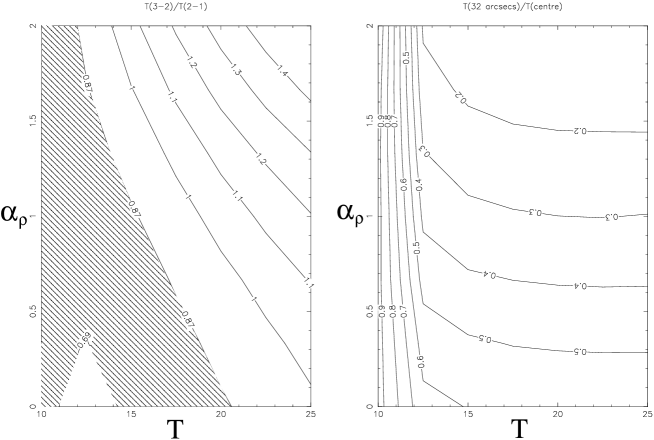
Figure 5: Two contour plots illustrating the effects of varying $\alpha_{\rho}$ and T, whilst setting $\alpha_{T}=\alpha_{\chi}=0$ (i.e. isothermal models). (a) Contours of the values of the ratio of $\rm T_{mb}$(J=3$\rm\rightarrow$2) to $\rm T_{mb}$(J=2$\rm\rightarrow$1). The area of this plot that is consistent with the data shown in Figures 1 & 2 is shaded. (b) Contours of the values of the ratio of $\rm T_{mb}$ at a radius of 32 arcsec from the centre to $\rm T_{mb}$ at core centre for the C¹⁸O (J=2$\rightarrow$1) transition. The value observed in the L1689B data for this ratio was 1.0$\pm$0.1. No physically realistic value of $\alpha_{\rho}$ can reproduce this value of the ratio.

The code starts by setting the population levels of the C¹⁸O rotationally excited states to be consistent with the Boltzmann distribution. The equation of radiative transfer is then numerically solved to obtain $\rm I_{\nu}$, the radiation field in each shell. Using this radiation field the rate equation is then solved to give a new, modified set of population levels. The procedure of calculating $\rm n_{J}$ (the population levels of the C¹⁸O) followed by $\rm I_{\nu}$ (the radiation field) is repeated until a stable solution is approached and convergence is achieved. The code can then solve the radiative transfer equation for lines of sight through the cloud and simulate observed line profiles by smoothing with a Gaussian spatial profile similar to the beam profile of the JCMT. The $\rm H_{2}$ collision rates for the model were obtained from Flower & Launey (1985), who calculated the collision rates for para-$H_{2}$ up to the $\rm J=11$ rotational level, for temperatures between 10 and 250K, and for ortho-$H_{2}$ up to the $\rm J=6$ level between 10 and 100K.

Throughout the simulations (unless stated otherwise) the model core representing L1689B had the following properties: The model core consisted of 20 logarithmically spaced shells (giving increased resolution towards the centre of the core), and a critical radius $\rm r_{crit}=0.02pc$ marking the boundary between the core and envelope. The micro-turbulent velocity component for each shell throughout the cloud was given by $\rm\delta v(r)\propto r^{0.3}$, up to a maximum 0.8 kms^-1 at the outside. This was chosen to be consistent with the observations summarised by Larson (1981) and to fit the observed line widths. The ortho- to para-$H_{2}$ ratio was fixed at 1.

The following section investigates the effect of varying the free parameters in the model of L1689B: $\rm\alpha_{T}$; $\rm\alpha_{\rho}$; $\rm\alpha_{\chi}$; and $\rm T_{outer}$. The central density, $\rm\rho_{c}$, was normalized in the simulations so as to reproduce the central brightness of the core in the (2$\rightarrow$1) transition.

4 Model Results

4.1 Isothermal Models

The simplest models of cloud cores assume a constant temperature. So we first investigate how the predicted appearance of L1689B is dependent on the inner core radial density profile $\rm\rho\propto r^{-\alpha_{\rho}}$ if a single temperature, T (=T_outer), exists throughout the core. In other words, we set both $\alpha_{T}$ and $\alpha_{\chi}$ to zero. Hence, the predicted appearance for the set of cores with temperatures between 10 and 25K and $\rm\alpha_{\rho}$ between 0 and 2 was calculated. By the nature of this form of modelling, we can run whole families of models and produce large output data-sets. We then illustrate these models as a series of contour plots in the two-dimensional phase space of the two parameters we are varying.

Figure 5 shows two contour plots that illustrate the effects of varying $\alpha_{\rho}$ and T. Figure 5(a) shows contours of the values of the ratio of $\rm T_{mb}$(J=3$\rm\rightarrow$2) to $\rm T_{mb}$(J=2$\rm\rightarrow$1). The area of this plot that is consistent with the data shown in Figures 1 & 2 is shaded. Figure 5(b) shows contours of the values of the ratio of $\rm T_{mb}$ at a radius of 32 arcsec from the centre to $\rm T_{mb}$ at core centre for the C¹⁸O (J=2$\rightarrow$1) transition. As noted in section 2 above, the value observed in the data of L1689B for this ratio was 1.0$\pm$0.1. It can be seen from Figure 5(b) that for T$>$13K this value increases as $\alpha_{\rho}$ decreases and that the brightness profile in this area is mainly dependent on the density profile of the core. However for T$<$13K the brightness profile becomes strongly dependent on T. This is because the C¹⁸O transitions become increasingly optically thick.

The reason why the (J=3$\rightarrow$2) to (J=2$\rightarrow$1) brightness ratio of the model core increases with both T and $\rm\alpha_{\rho}$ is because the upper rotational levels of C¹⁸O become more populated as the temperature and density increase. It should be noted that the singular isothermal sphere model represents the upper border of Figure 5(b). This is the part of the plot furthest from consistency with the data for T$>$13K. This agrees with the conclusions of Papers I & II that L1689B does not represent the singular isothermal sphere initial conditions for star formation.

Although at first sight setting T=10K seems to offer a possible explanation for L1689B’s brightness profile, another effect led us to reject this as a possible model for L1689B. At 10K the model has very high optical depths and the predicted line profiles are significantly wider and show an extended ‘flat top’. This is illustrated in Figure 6. The central C¹⁸O line profile is shown as observed (the data points) and as predicted by the model $\alpha_{\rho}$=0, T=12K (solid line) and $\alpha_{\rho}$=0, T=10K (dashed line). It is clear that the T=10K model does not agree with the data. We therefore need to find some other mechanism to explain the low contrast observed in the data.

Figure 6: Comparison of observed C¹⁸O (J=2$\rm\rightarrow$1) line (data points) with two isothermal models. The first model (solid line) has T=12K, the second (dashed) has T=10K. The second clearly shows a flat top due to high optical depths, and is not consistent with the data.

4.2 Varying temperature models

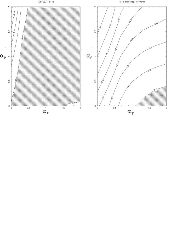
Figure 7: Two contour plots illustrating the effects of varying $\alpha_{\rho}$ and $\alpha_{T}$ simultaneously. (a) Contours of the values of the ratio of $\rm T_{mb}$(J=3$\rm\rightarrow$2) to $\rm T_{mb}$(J=2$\rm\rightarrow$1). The shaded area is consistent with the L1689B data. (b) Contours of the values of the ratio of $\rm T_{mb}$ at a radius of 32 arcsec from the centre to $\rm T_{mb}$ at core centre for the C¹⁸O (J=2$\rightarrow$1) transition. The shaded area is consistent with the data from Figures 1 & 2. Note that the two shaded areas overlap slightly.

We next investigated a set of models in which the outer envelope was at a temperature of 20K, but in the inner region the temperature profile falls as $\rm T\propto r^{\alpha_{T}}$ to a minimum temperature of 10K. This means that, when $\rm\alpha_{T}$ is greater than approximately 0.5, an inner 10K region is created, whose size increases as $\rm\alpha_{T}$ rises. When $\rm\alpha_{T}$ is 2.0, the radius of this region is 0.015pc.

Figure 7 shows two contour plots that illustrate the effects of varying $\alpha_{\rho}$ and $\alpha_{T}$ simultaneously. Figure 7(a) shows contours of the values of the ratio of $\rm T_{mb}$(J=3$\rm\rightarrow$2) to $\rm T_{mb}$ (J=2$\rm\rightarrow$1). The area of this plot that is consistent with the L1689B data is shaded.

Figure 7(b) shows contours of the values of the ratio of $\rm T_{mb}$ at a radius of 32 arcsec from the centre to $\rm T_{mb}$ at core centre for the C¹⁸O (J=2$\rightarrow$1) transition. As noted in section 2 above, the value observed in the data of L1689B for this ratio was 1.0$\pm$0.1. Once again the part of this plot that is consistent with the data from Figures 1 & 2 is shown as a shaded area on Figure 7(b). The fact that figure 7(b) shows a much larger variation than Figure 7(a) illustrates the importance of taking observations at more than one radius if one wishes to truly characterize cloud cores, and shows clearly that single spectra at the centre of a cloud do not constrain its parameters.

This time there is a set of values of $\alpha_{\rho}$ and $\alpha_{T}$ that is consistent with all of the C¹⁸O data. This approximately corresponds to $1.1<\alpha_{T}<2$ and $0<\alpha_{\rho}<0.4$. However, at the 1$\sigma$ level, we can also say that if $\alpha_{\rho}\leq 0.1$, then $\alpha_{T}$ must by $\leq 1.5$. These results reveal that a decrease in temperature towards the centre of the core does indeed help to explain the C¹⁸O appearance of L1689B. In fact a model which has a flat inner density profile and a very steep temperature drop from 20K at a radius of 0.02pc, to 10K at a radius of 0.015pc, is consistent with our observations.

Figure 8: Sketch of the assumed observing geometry of L1689B.

4.3 Continuum data revisited

A 1.3-mm continuum map of L1689B was published in Paper II. In this section we incorporate those observations to see what further constraints we can place on our model of L1689B. Remembering that the millimetre continuum arises from thermal emission from dust grains, the flux density in this situation (e.g. Hildebrand 1983) is given by:

$$S_{\nu}=B_{\nu}(T)\Omega(1-e^{-\tau_{\nu}}),$$ (2)

where $B_{\nu}(T)$ is the black-body function at temperature $T$, $\Omega$ is the source solid angle and $\tau_{\nu}$ is the optical depth. This form is often referred to as a grey-body function. The black-body function can often be simplified to the so-called Rayleigh-Jeans approximation in cases where $(h\nu/kT)<<1$. However, at 1.3 mm, $(h\nu/k)=10.8K$, which is within a factor of 2 of our fitted temperature for the the L1689B core (see above). Hence, in this case the Rayleigh-Jeans approximation may introduce errors, so we here outline a somewhat more rigorous approach.

Figure 8 shows our assumed observing geometry. We still make the assumption that the dust properties, such as grain size distribution, abundance with respect to H₂ and emissivity, are constant throughout the cloud. Then we see that the intensity arising from an element of the cloud of length $dx$ at a given frequency is:

$$dI(x)\propto\rho(x)B(T(x))dx,$$ (3)

where $\rho(x)$ is the density profile along the line of sight and $T(x)$ is the temperature profile of the dust along the line of sight – see Figure 8.

Figure 9: Contours of the values of the ratio of $\rm T_{mb}$ at a radius of 32 arcsec from the centre to $\rm T_{mb}$ at core centre for the C¹⁸O (J=2$\rightarrow$1) transition. The shaded area at lower right is consistent with the data from Figures 1 & 2. The shaded strip towards the upper left indicates the constraints placed on $\alpha_{T}$ and $\alpha_{\rho}$ by the continuum data. Note that the two shaded areas do not overlap.

The simple form often used for power-law radial profiles, is that if $T(r)\propto r^{-q}$, $\rho(r)\propto r^{-p}$, and the flux density $S_{\nu}(\theta)\propto\theta^{-m}$ then the indices are related by the simple expression $m=p+q-1$ (Casali 1986, Adams 1991). This is derived by assuming the depth of the cloud remains constant across the entire core (e.g. a slab or infinite cloud). However, this form only holds for the Rayleigh-Jeans approximation, and for the case where the radial density and temperature each follows a single power-law, and there is no break in the power laws, such as we have in our model – see Figure 4. We derive below a more rigorous set of relations.

If the density profile $\rho(r)$ and the temperature profile $T(r)$ are known, where r is the radial distance from the cloud centre, then the observed surface brightness I(R) is given by the equation of radiative transfer in the assumption of optically thin emission:

$$I(R)\propto\int_{-x_{0}}^{+x_{0}}\rho(r)B(T[r])dx.$$ (4)

Making the substitutions $R=r\cos\theta$ and $dx=[Rd\theta/\cos^{2}\theta]$ we derive:

$$I(R)\propto R\int_{-\cos^{-1}(R/R_{c})}^{\cos^{-1}(R/R_{c})}\rho(R/\cos\theta)\ B(T[R/\cos\theta])\frac{d\theta}{\cos^{2}\theta}.$$ (5)

For the model of L1689B, the density profile in the outer envelope is represented by the power law $\rho\propto r^{-2}$. Hence, for $R>r_{crit}$ (i.e. for observations of the outer envelope) we have:

$$I(R)\propto R^{-1}\int_{-\pi/2}^{\pi/2}(\cos\theta)^{-4}d\theta,$$ (6)

where the limits in the integration have been set using the approximation that the core extends to infinity. This integral is independent of R and therefore we predict the $I(R)\propto R^{-1}$ behaviour in the envelope of L1689B that was actually observed in the continuum in Paper II.

However, for the inner core the equation for the projected surface brightness becomes more complicated:

$$I(R)\propto\frac{B(T_{env})}{\omega}\left(\frac{\pi}{2}\cos^{-1}(\omega)\right)+$$

$$\omega\int_{0}^{\cos^{-1}(\omega)}\frac{\omega^{-\alpha_{\rho}}B\left(T_{env}\omega^{-\alpha_{T}}cos^{\alpha_{T}}\theta\right)cos^{\alpha_{\rho}}\theta}{cos^{2}\theta}d\theta,$$

where we have used the substitution $\omega=R/r_{crit}$, and $\rm T_{env}$ is the envelope temperature. The first term of this equation is the contribution to the signal from the envelope, while the second term is the contribution from the core. This equation can be solved numerically for any value of $\alpha_{\rho}$ or $\alpha_{T}$, to predict the brightness profile I(R).

Numerical solution of equation 7 in the isothermal case allows us to compare the continuum radial flux density variation observed in Paper II, with that predicted by the parameterised model we have presented here. We find that models with $\rho\propto r^{-0.5\pm 0.1}$ (i.e. $\alpha_{\rho}=0.5\pm 0.1$) best match the data presented in Paper II. A more general, non-isothermal, solution to the continuum appearance of L1689B can be expressed approximately as:

$$\alpha_{\rho}-1.5\alpha_{T}=0.5\pm 0.1.$$ (8)

This solution was found by numerically solving equation 7 for all values of $\alpha_{\rho}$ between 0 and 2, and $\alpha_{T}$ between 0 and 2, and then finding which range of values give solutions best matching the data in Paper II. This is a new and different constraint to that discovered in the above modelling of the C¹⁸O data.

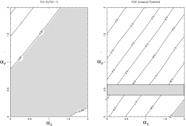
Figure 10: Two contour plots illustrating the effects of varying $\alpha_{\rho}$ and $\alpha_{\chi}$ simultaneously. (a) Contours of the values of the ratio of $\rm T_{mb}$(J=3$\rm\rightarrow$2) to $\rm T_{mb}$(J=2$\rm\rightarrow$1). The shaded area is consistent with the L1689B CO data. (b) Contours of the values of the ratio of $\rm T_{mb}$ at a radius of 32 arcsec from the centre to $\rm T_{mb}$ at core centre for the C¹⁸O (J=2$\rightarrow$1) transition. The shaded area at the lower right hand corner is consistent with the data from Figures 1 & 2. The horizontal shaded strip indicates the constraints placed on $\alpha_{\rho}$ by the continuum data.

Figure 9 illustrates this additional constraint introduced by the continuum data by reproducing the contours from Figure 9(b) – the values of the ratio of $\rm T_{mb}$ at a radius of 32 arcsec from the centre, to $\rm T_{mb}$ at core centre for the C¹⁸O (J=2$\rightarrow$1) transition – as a function of varying $\alpha_{\rho}$ and $\alpha_{T}$. Once again the part of this plot that is consistent with the CO data from Figures 1 & 2 is shown as a shaded area on Figure 7(b). However, now we have added an additional shaded strip at the upper left of the plot illustrating the constraint placed by the continuum data, as described by equation 8. We see that the two shaded areas do not overlap, indicating that there is no simultaneous fit to the CO data and the continuum data. Hence, a more complex model is required to simultaneously fit all of the data.

4.4 Varying the CO abundance

The simplest way to try to reconcile the CO data to the continuum data is to vary the abundance of gas-phase CO relative to H₂. This is predicted to occur in regions of high density, as the CO freezes out onto the dust grains, and it has been observed qualitatively in many regions on many occasions (e.g. Mezger et al. 1990; Gibb & Little 1998; Ward-Thompson et al. 2000). It is thought to occur at temperatures less than 17K (Nakagawa 1980, Bergin & Langer 1997). So we ran a set of models to investigate the effect of decreasing the CO abundance towards the centre of the core. These models had a single temperature of 20K, an inner density gradient as before, of $\rho\propto r^{-\alpha_{\rho}}$, and a CO abundance fraction $\chi\propto r^{\alpha_{\chi}}$. We then investigated the regime $0<\alpha_{\rho}<2$ and $0<\alpha_{\chi}<2$.

Figure 10 shows two contour plots that illustrate the effects of varying $\alpha_{\rho}$ and $\alpha_{\chi}$ simultaneously. Figure 10(a) shows contours of the values of the ratio of $\rm T_{mb}$(J=3$\rm\rightarrow$2) to $\rm T_{mb}$(J=2$\rm\rightarrow$1). The area of this plot that is consistent with the CO data is shaded.

Figure 10(b) shows contours of the values of the ratio of $\rm T_{mb}$ at a radius of 32 arcsec from the centre to $\rm T_{mb}$ at core centre for the C¹⁸O (J=2$\rightarrow$1) transition. As noted in section 2 above, the value observed in the data of L1689B for this ratio was 1.0$\pm$0.1. Once again the part of this plot that is consistent with the data from Figures 1 & 2 is shown as a shaded area in the lower right hand corner of Figure 10(b).

Including the continuum data in this case, with $\alpha_{T}=0$, equation 10 simplifies to $\alpha_{\rho}=0.5\pm 0.1$. Figure 10(b) illustrates this additional constraint as an horizontal shaded strip in the lower half of the plot. Again we see that the two shaded areas do not overlap, indicating that there is no simultaneous formal fit to the CO data and the continuum data. However, this is only at the 1$\sigma$ level, and we find that the shaded regions would overlap at the 2$\sigma$ level for the values $\alpha_{\chi}\sim 1.9-2$ and $\alpha_{\rho}\sim 0.4$. This abundance effect is quite extreme – it implies a 95% drop in C¹⁸O abundance from edge to centre – although not unprecedented. Gibb and Little (1998) found a similar reduction in the C¹⁸O abundance in HH23–26.

Furthermore, if there is such a large amount of freeze-out taking place, this will increase the average grain size towards the core centre and consequently the dust grain mass opacity. In this case we would over-estimate the central density profile exponent, $\alpha_{\rho}$ derived from the continuum data. This would then act to shift the horizontal shaded region in Figure 10(b) downwards, causing a genuine overlap region at the 1-$\sigma$ level. Thus we have a fit to the data with $\alpha_{\chi}\sim 2$ and $\alpha_{\rho}\leq 0.4$. The spectra produced by the model were compared with those observed and there was good agreement within the errors. This is an isothermal fit. However we cannot rule out a slight temperature gradient, depending upon how much the dust opacity parameters that are not well constrained can vary.

We ran this set of simulations for several temperatures from 10 to 25K. We found that the predicted surface brightness did not vary significantly with T, even at very low temperatures. However, the predicted ratio of C¹⁸O (J=3$\rightarrow$2) to C¹⁸O (J=2$\rightarrow$1) did fall with T, and for models with T$<$14K the predicted values were too low to match our observations.

4.5 Other factors

There are other factors than those discussed above that may affect the conclusions of the modelling. One such factor is that the ortho- to para-H₂ ratio in these cores is not well defined. Since ortho-H₂ has a higher cross section for collisions with CO, the ratio of ortho- to para-H₂ may affect the conclusions drawn. It was found that by increasing the fraction of ortho-H₂, the C¹⁸O centre-to-edge ratio increased. However, it hardly affected the ratio of the the (J=3$\rightarrow$2) to (J=2$\rightarrow$1) transitions. Varying the ortho- to para- ratio altered the centre-to-edge ratio by 0.1 at most.

Similarly, the precise form of the microturbulence profile may influence the appearance of the core. For example, it was found that when using a constant $\delta v$ microturbulence profile, the brightness gradient decreased slightly – T(32 arcsec)/T(centre) increased by $\sim$ 0.1. However, neither of these two factors affected the appearance of the L1689B data strongly enough to affect the conclusions drawn above.

The geometry of the core as a whole may also change the exact form of the solutions. In particular, any departure from spherical symmetry would have an effect. Likewise, any variations from homogeneity – i.e. clumpiness within the core – is also likely to affect the predicted appearance of the core in mm/submm observations. It is difficult to quantify these effects, and further data would be needed to constrain these extra parameters.

We also investigated the possible effect of having a small temperature gradient in the envelope, or allowing the density gradient in this region to fall less steeply ($\rho\propto n^{-1.7}$). This was found to only vary the ratio of T(32 arcsec)/T(centre) by $\sim$ 0.05. Checks to ensure that the exact values of the inner radius, and the cloud size did not significantly affect our results were also made.

5 Conclusions

In this paper we have presented new C¹⁸O (J=3$\rightarrow$2) and (J=2$\rightarrow$1) data of the pre-stellar core L1689B. We have used a spherically symmetric radiative transfer code to model these data in terms of three parameters – the gradients in temperature, density and C¹⁸O abundance. In the three dimensional parameter space defined by the three exponents, $\alpha_{\rho}$, $\alpha_{T}$, and $\alpha_{\chi}$, we have found solutions consistent with the data. There is a region defined by $\alpha_{\rho}-1.5\alpha_{T}=0.5\pm 0.1$, which is consistent with the mm continuum observations of L1689B.

There is also a set of solutions that can simultaneously predict the molecular CO appearance and the mm continuum data, implying $\alpha_{\rho}\leq 0.4,\alpha_{T}=0$ (although this is not well constrained) and $\alpha_{\chi}=2$. Hence, we have shown that there is freeze-out of CO towards the centre, and we have constrained the radial density and temperature profiles. Thus we have shown that the combination of mm/submm spectral line and continuum data, with a rigorous treatment of radiative transfer, is a powerful method of investigating the physics of pre-stellar evolution.

References

- [1] Adams F. C., ApJ, 382, 544
- [] André P., Ward-Thompson D., Motte F., 1996, A&A, 314, 625 – Paper II
- [] Bacmann A., André P., Puget J-L., Abergel A., Bontemps S., Ward-Thompson D., 2000, A&A, in press
- [Beichmann et al. 1986] Beichman C. A., Myers P. C., Emerson J. P., Harris S., Mathieu J. P., Benson P. J., Jennings R. E., 1986, ApJ, 307, 337
- [Benson et al. 1989] Benson P. J., Myers P. C., 1989, ApJS, 71, 89
- [] Bergin E. A., Langer W. D., 1997, ApJ, 486, 316
- [] Casali M. M., 1986, MNRAS, 223, 341
- [] Cunningham C. T., Hayward R. H., Wade J. D., Davies S. R., Matheson D. N., 1992, Int. J. Infrared Millimetre Waves, 13, 1827
- [] Davies S. R., Cunningham C. T., Little L. T., Matheson D. N., 1992, Int. J. Infrared Millimetre Waves, 13, 647
- [] Flower D. R., Launey J. M., 1985, MNRAS, 214, 275
- [] Gibb A. G., Little L. T., 1998, MNRAS, 295, 299
- [Hildebrand 1983] Hildebrand R. H., 1983, QJRAS, 24, 267
- [] Kutner M. L., Ulich B. L., 1981, ApJ, 250, 341
- [] Larson R. B., 1981, MNRAS, 194, 809
- [] MacLaren I., Richardson K. M., Wolfendale A. W., 1988, ApJ, 333, 821
- [] Matthews H. E., 1999, ‘JCMT Guide for Prospective Users’, JAC, Hawaii
- [] Matthews N., 1986, PhD thesis, University of Kent
- [] Mezger P. G., Zylka R., Wink J.-E., 1990, A&A 228, 95
- [] Nakagawa N., 1980, in: Andrew B. H., ed., ‘Interstellar Molecules’
- [] Padman R., 1990, ‘Specx Users Manual’, MRAO, University of Cambridge
- [] Shu F. H., 1977, ApJ, 214, 488
- [] Stenholm, L. G., 1977, A&A, 54, 577
- [] Tafalla M., Mardones D., Myers P. C., Caselli P., Bachiller R., Benson P. J., 1998, ApJ, 504, 900
- [] Ward-Thompson D., Motte F., André P., 1999, MNRAS, 305, 143 – Paper III