Galaxy Cluster Gas Mass Fractions from Sunyaev-Zel’dovich Effect Measurements: Constraints on $\Omega_{M}$

Abstract

Using sensitive centimeter-wave receivers mounted on the Owens Valley Radio Observatory and Berkeley-Illinois-Maryland-Association millimeter arrays, we have obtained interferometric measurements of the Sunyaev-Zel’dovich (SZ) effect toward massive galaxy clusters. We use the SZ data to determine the pressure distribution of the cluster gas and, in combination with published X-ray temperatures, to infer the gas mass and total gravitational mass of 18 clusters. The gas mass fraction, $f_{g}$, is calculated for each cluster, and is extrapolated to the fiducial radius $r_{500}$ using the results of numerical simulations. The mean $f_{g}$ within $r_{500}$ is $0.081^{+0.009}_{-0.011}h^{-1}_{100}$ (statistical uncertainty at 68% confidence level, assuming $\Omega_{M}$=0.3, $\Omega_{\Lambda}$=0.7). We discuss possible sources of systematic errors in the mean $f_{g}$ measurement.

We derive an upper limit for $\Omega_{M}$ from this sample under the assumption that the mass composition of clusters within $r_{500}$ reflects the universal mass composition: $\Omega_{M}h\leq\Omega_{B}/f_{g}$. The gas mass fractions depend on cosmology through the angular diameter distance and the $r_{500}$ correction factors. For a flat universe ($\Omega_{\Lambda}$$\equiv$ 1 - $\Omega_{M}$) and $h=0.7$, we find the measured gas mass fractions are consistent with $\Omega_{M}$ less than 0.40, at 68% confidence. Including estimates of the baryons contained in galaxies and the baryons which failed to become bound during the cluster formation process, we find $\Omega_{M}$ $\sim$0.25.

1 Introduction

Clusters of galaxies, by virtue of being the largest known virialized objects, are important probes of large scale structure and can be used to test cosmological models. Rich clusters are extremely massive, $\sim$$\ 10^{15}M_{\odot}$, as indicated by the presence of strongly gravitationally lensed background galaxies, the large velocity dispersion ($>$ 1000 km s^-1) in the member galaxies, and the high measured temperature ($>5$ keV) of the ionized intracluster gas. The mass composition on cluster mass scales is expected to reflect the universal mass composition (White et al. 1993; Evrard 1997) . Under the fair sample assumption, then, the cluster gas mass fraction, which is a lower limit to the cluster’s baryon fraction, $f_{B}$, should reflect the universal baryon fraction:

$$f_{g}\leq f_{B}\equiv{\Omega_{B}\over\Omega_{M}},$$ (1)

where $\Omega_{B}$ is the ratio of baryon mass density in the universe to the critical mass density. The cluster gas mass fraction measurement can be used within the Big Bang Nucleosynthesis (BBN) paradigm to constrain $\Omega_{M}$,

$$\Omega_{M}\leq\Omega_{B}/f_{g}.$$ (2)

The value of $\Omega_{B}$ is constrained by BBN calculations and the measurements of the abundances of the light elements (Wagoner et al. 1967; Copi et al. 1995) as well as measurements of the spatial anisotropies of the cosmic microwave background (CMB) (White et al. 1994; Hu et al. 1997).

The luminous baryons in clusters are mainly in the gaseous intracluster medium (ICM). The gas mass is about an order of magnitude larger than the mass in optically observed cluster galaxies, e.g., White et al. (1993); Forman & Jones (1982). Hence, the gas mass is not only a lower limit to the cluster’s baryonic mass, it is a reasonable estimate of it. Although observations suggest that galaxy groups and low mass clusters may have lost gas due to preheating or post-collapse energy input (David et al. 1995; Mohr et al. 1999; Ponman et al. 1996), the gas mass fraction in massive clusters ($T_{e}>5$ keV) appears to be constant. The gas mass fraction in massive clusters then provides a lower limit to the cluster baryon fraction, $f_{g}\leq f_{B}$.

The ICM is hot, with electron temperatures, $T_{e}$, from $\sim$5 to 15 keV; rarefied, with peak electron number densities of $n_{e}\simeq 10^{-3}$ ${\rm cm}^{-3}$; and cools slowly ($t_{cool}>t_{Hubble}$), mainly via thermal Bremsstrahlung in the X-ray band. The ICM also produces a spectral distortion of the CMB known as the Sunyaev-Zel’dovich effect. The ICM mass fraction may be calculated from either of these observables. In addition to providing measurements of this important parameter with independent techniques, the two methods are fundamentally different in that the SZ effect is directly proportional to the integrated density of the gas while the X-ray brightness is proportional to the integrated square of the density.

The X-ray surface brightness is proportional to the emission measure, $S_{x}\propto\int n_{e}^{2}\Lambda(T_{e})dl$, where the integration is along the line of sight. Under simplifying assumptions, the gas mass can be calculated from an X-ray image deprojection. Since the sound crossing time of the cluster gas is typically much less than the dynamical time, one may reasonably assume that, in the absence of a recent merger, the cluster gas is relaxed in the cluster’s potential. Hydrodynamic simulations support this notion, e.g., Evrard et al. (1996). Under the assumption that the gas is in hydrostatic equilibrium (HSE), supported only by thermal pressure, the total binding mass follows from the gas density and temperature distribution, the latter of which may be determined with X-ray spectra. Gas mass fractions have been measured with this technique out to cluster radii of 1 Mpc or more (White & Fabian 1995; David et al. 1995; Neumann & Böhringer 1997; Squires et al. 1997; Mohr et al. 1999). In an X-ray flux-limited sample of 45 clusters, Mohr et al. (1999) measure the mean cluster gas mass fraction within approximately the virial radius to be (0.0749 $\pm 0.0005)h^{-3/2}$. Here, and throughout the paper, we use $H_{\circ}=100h$ km s^-1 Mpc^-1.

In this work, we calculate cluster gas mass fractions using spatially resolved measurements of the SZ effect to determine the gas density profile. The SZ effect in clusters is a spectral distortion of the CMB radiation due to inverse-Compton scattering of the relatively cool CMB photons off hot ICM electrons (Sunyaev & Zel’dovich 1972). At frequencies less than $\sim$  218 GHz, the intensity of the CMB radiation is diminished as compared to the unscattered CMB, and the SZ effect is manifested as a brightness temperature decrement towards the cluster. This decrement, $\Delta T_{SZ}/T_{CMB}$, has a magnitude proportional to the Compton $y$-parameter, i.e., the total number of scatterers, weighted by their associated temperature,

$$y={{k\sigma_{T}}\over{m_{e}c^{2}}}\int{n_{e}(l)T_{e}(l)dl},$$ (3)

where $k$ is Boltzmann’s constant, $\sigma_{T}$ is the Thomson scattering cross section, $m_{e}$ is the electron mass. We extract the cluster’s gas mass fraction from a deprojection of the SZ effect data in a method analogous to the described X-ray HSE analysis.

In addition to providing an additional measurement of $f_{g}$, we note several points of difference between the X-ray and SZ analyses. Should significant large-scale or spatially-varying clumping of the ICM be present, the SZ image deprojection may look quite different from the X-ray deprojection. Clumping at scales below the resolution of the X-ray and SZ images could also result in a difference of $<n_{e}^{2}>^{1/2}/<n_{e}>$ in the inferred gas mass. Also, the emission from the cores of relaxed clusters may be dominated by cooling flows, which complicate the interpretation of the X-ray data and may bias the result strongly if not taken into account (Allen & Fabian 1998; Mohr et al. 1999). The direct relationship between the SZ effect and the gas density also permits a surface gas mass fraction to be measured without image deprojection by comparing the projected or “surface” gas mass from the SZ observation to a measurement of the surface total cluster mass, for instance from gravitational lensing models (cf Grego et al. (2000)). Because lensing observations are not available for all the clusters in our sample, and because we are interested in the gas mass fraction within clearly defined cluster radii, for this work we calculate $f_{g}$ with the deprojection/HSE method only.

In this paper, we present cluster gas mass fractions based on SZ measurements made in the years 1994-1998, and a discussion of the implications of these measurements for cluster physics and for cosmology. In previous papers (Carlstrom et al. 1996; Grego et al. 2000), we have described the instrument constructed expressly to make such measurements, and the reduction and calibration methods for the SZ measurements. We give a brief review of this and discuss the cluster selection and observations in Section 2. In Section 3, we describe the procedure for fitting the SZ data to models for the cluster gas and extracting cluster gas masses and gas mass fractions, including a discussion of the possible systematic uncertainties. In Section 4 we present the derived gas masses and gas mass fractions for the entire cluster sample, compare these results to other gas mass fraction work, and discuss the limits this work places on $\Omega_{M}$ and plans for future work.

2 Instrument and Observations

2.1 An Overview of the OVRO and BIMA 30 GHz SZ Observations

We wish to take advantage of the characteristically low noise of interferometer systems while retaining sensitivity on the large angular scales subtended by clusters. To do this, we integrated centimeter-wave receivers built expressly for this purpose into the millimeter-wavelength interferometer systems at the Owens Valley Radio Observatory (OVRO) Millimeter Array and at the Berkeley-Illinois-Maryland Association (BIMA) Millimeter Array. The angular scale sampled by an interferometer element is $\theta\sim\lambda/B$, where $B$ is the projected baseline, or telescope spacing as seen by the source. At our $\sim$ 1 centimeter operating wavelength, the compact telescope configurations effectively sample the angular scales of clusters while the fluxes of any contaminating pointlike sources in the field are simultaneously monitored with the longer baselines, so their time variability is not a source of uncertainty. Operating the millimeter systems at $\sim 10$ times lower frequency than the design frequency also provides for very good optical performance. Both arrays allow for the elements to be placed in a wide variety of configurations.

The receivers, which operate from 26 to 36 GHz, are based on cryogenically-cooled 4-stage HEMT amplifiers and achieve receiver temperatures of 12-20 K at 28.5 GHz. Results from this system are reported in Carlstrom et al. (1996, 2000); Grego et al. (2000); Holzapfel et al. (2000a, b); Patel et al. (2000); Reese et al. (2000).

2.2 The Interferometric Arrays

We observed with this system at the OVRO Millimeter Array in the summers of 1994-1996 and 1998. At OVRO, the weather was adequate for observing about 80% of the time. The aperture efficiency at 28.5 GHz, $\simeq$ 0.75, was measured with holographic techniques. The contribution of the antenna to the system temperature, including spillover, is $\simeq$ 12-15 K, as measured from sky dips. The array of six 10.4 meter telescopes (four telescopes in 1994) is two-dimensional, with baselines ranging from 14 to 240 meters. A general description of the OVRO millimeter array is provided in (Padin et al. 1991). The continuum measurements are made with the dual-channel analog correlator, each channel having an input bandwidth of 1 GHz. In 1994, the SZ observations were made using a single channel centered at 28.7 GHz. After 1994, the observations were made in single-sideband mode using two 1 GHz channels, centered at 28.5 and 30 GHz. At OVRO’s latitude, sufficient $u$-$v$ coverage can be obtained for sources with declinations greater than $-10^{\circ}$ when two or three different telescope configurations are used. The primary beams for each telescope are measured holographically and are quite similar. The full width at half maximum (FWHM) of the beams differ maximally by five percent, and can be approximated as Gaussian with a FWHM of 252^′′.

We used the same receiver system at the BIMA Millimeter Array in the summers of 1996, 1997, and 1998. In 1996, we used the six receivers on six of the BIMA telescopes; three additional receivers were constructed to use a total of nine of the ten BIMA telescopes in the summers of 1997 and 1998. At BIMA, the contribution to the system temperature from the antenna is minimal, $\sim$ 6 K. The aperture efficiency at 30 GHz with our receivers is $\sim$ 0.70. The BIMA array is two-dimensional, with baselines ranging from as short as 7.5 meters and as long as 1 kilometer. A general description of the BIMA interferometer is given in (Welch et al. 1996). We operate the hybrid digital correlator in wideband mode (mode 8 in the notation of Welch et al. (1996)) covering 800 MHz with 2-bit sampling. Adequate $u$-$v$ coverage can be obtained for sources with declinations greater than about $-10^{\circ}$ with one or two telescope configurations. The primary beams for each telescope were measured holographically and are very similar. The FWHM of the beams differ maximally by $\sim$3% and can be approximated by Gaussian with a $396^{\prime\prime}$ FWHM.

2.3 Data Reduction and Calibration

2.3.1 OVRO Reduction

Our observing strategy maximized usable observing time on the cluster while also providing reliable instrument calibration. During times the cluster was observable with minimal shadowing, we interleaved twenty-four minute observations of the cluster with observations of a nearby bright radio source (the gain calibrator) to monitor the stability of the interferometer’s phase and amplitude response. The cluster and gain calibrator observations were taken in several short segments (four and one minute integrations, respectively) to minimize the effect of short-term instabilities on observing efficiency. Either a planet or a time-stable bright radio source was observed to provide the absolute flux scale for the measurement. This flux scale is based on Mars; if Mars was at least $15^{\circ}$ above the horizon during the cluster observation, it was observed.

The data were edited according to several criteria. Data taken with a telescope which was blocked by another telescope (shadowed) are removed from the data set. We use a conservative shadowing limit; data are discarded if the projected baseline is less than 1.05 times the telescope diameter. Also removed are data taken during poor weather as evidenced by poor phase stablity and data affected by anomalous jumps in the instrument’s phase. Any cluster data not bracketed by calibrator observations are also removed.

Data calibration proceeds in two steps, gain calibration and absolute flux calibration. A time series of the gain calibrator’s amplitude and phase in each baseline is examined with the MMA data reduction package (Scoville et al. 1993). The instrument response during the cluster observations is interpolated from a fit to this time series. The amplitude response generally varied less than a percent over an observation of many hours. The average gains for each baseline were quite stable from day to day. In the 1994 and 1995 observing seasons, however, the receivers responded to linearly polarized light. Since some of the gain calibrators are linearly polarized at the 5-10% level, the measured amplitude of such calibrators changes with parallactic angle as well as instrument response. Only a few of the cluster observations are significantly affected, since two different gain calibrators were often used for a single cluster and in no case were both noticeably polarized. For the affected clusters, the average calibrator flux is used and the amplitude gain is assumed to be constant. The instrumental phase response typically only drifts a few tens of degrees over the course of a cluster observation.

The absolute flux scale is determined relative to Mars. Mars’ brightness temperature is predicted using a radiative transfer model for the whole disk brightness temperature (Rudy 1987) for each day of observation. The intrinsic uncertainty of this model is expected to be $\sim 2.5\%$ and the uncertainty from input parameter uncertainties is about 3%, and so we estimate the accuracy of our absolute flux scale to be 4% at 90% confidence. We calculate the brightness temperature at the center frequency of our observed band; the brightness temperature varies less than a percent over our bandpass. The solid angle Mars subtends at each observation is determined from the equatorial and polar diameters of Mars reported in the Astronomical Almanac.

Goldin et al. (1997) compared the Rudy model to a thermal model for Mars, and find even with substantial extrapolations in wavelength, the two models predict brightness temperatures for Mars consistent with each other. We also compare the Mars brightness temperature predicted by the Rudy model to those derived by Mason et al. (1999) based on absolute flux measurements of Cas A. They find Mars’ brightness temparature at 32 GHz to be $196.0^{+7.5}_{-7.6}$ K for the May 1998 epoch. In our observing scheme, we determine the brightness temperature separately for each day. The brightness temperature predicted by the Rudy model at 32 GHz varies from 194 K to 203 K during the month of May 1998. The brightness temperature for Mars varies less than 0.2% between 28 and 30 GHz. These comparisons suggest that our primary calibration is accurate and is consistent with the primary calibration used by other groups.

The fluxes of a set of primary calibrators were determined using the predicted Mars flux. Since the amplitude gain of the instrument is stable with respect to time and telescope elevation, the observations of these calibrators and Mars need not be contiguous. In the case our primary calibrator is never observable at the same time as Mars, we bootstrap the flux from another primary calibrator. Over each of the month-long observation seasons, no time variation of the gain calibrator fluxes was evident.

2.3.2 BIMA Reduction

At BIMA, we use an observing scheme similar to that used at OVRO, interleaving observations of the gain calibrator and cluster.

The reduction proceeds much like the OVRO reduction with additional editing and passband calibration. Spectral channels with low signal-to-noise ratio or with spurious interference are discarded. Also edited out are shadowed data, data taken with obviously incorrect or irregular system temperatures, data taken when the telescope tracked incorrectly, and data contaminated by local interference. (These errors are flagged online at OVRO.) The spectral response of the instrument is determined from a passband calibrator, and then the spectral channels are vector averaged into one wideband channel. The gain calibration is then performed.

Absolute flux calibration at BIMA evolved between the 1997 and 1998 seasons. For the 1997 data, each of the Mars observations were reduced in the method described above, and the resultant amplitude and phase are SELFCALed. The amplitude response for each of the 9 telescopes is determined using the flux of Mars from the Rudy model. The gains were very stable over the two months of observing time, with an $r.m.s.$ antenna gain variation of 1.2% for all telescopes all summer. With the knowledge that the amplitude response is steady, in 1998 the gains were derived in the first week of the BIMA observations, and these gains are applied online. Mars was subsequently observed to monitor any gain variation.

2.4 Cluster Selection and Observations

We observed over 40 clusters with the centimeter-wave SZ system during the 1994-1998 observing seasons. Only some of these clusters were observed for a significant amount of time; some observations were intended to survey for point sources and to define a sample for future work. To date, over 25 clusters have been detected significantly; analysis of a sample of 18 are presented here.

The cluster targets were selected from a flux-limited, homogeneous sample of clusters (Stocke et al. 1991; Gioia & Luppino 1994; Nichol et al. 1997) identified from the Einstein Extended Medium Sensitivity Survey (EMSS) (Gioia et al. 1990) and from two flux-limited samples (XBACS, Ebeling et al. (1996); BCS, Ebeling et al. (1998)) from the ROSAT All-Sky Survey, as well as public ROSAT data. Identifying clusters based on X-ray emission rather than galaxy surface-density enhancements ameliorates the problems of false detections due to chance superpositions and of missed clusters due to smaller-than-average backgrounds.

We selected massive clusters for our sample. X-ray studies of clusters in David et al. (1995) and Mohr et al. (1999) indicate that the gas mass fraction near the virial radius increases as cluster mass increases, but that above $\sim 5$ keV the gas mass fraction at the virial radius is constant. At the initiation of this work, X-ray temperatures were not widely available for distant clusters. We chose instead to select clusters on the basis of luminosity. We expect a cluster’s X-ray luminosity to be a better predictor of mass than X-ray surface brightness, as it will be less sensitive to projection effects and contamination by cooling flows and dynamical activity in the ICM. Although cooling flows have been observed to contribute as much as 70% of a cluster’s luminosity, typically they only contribute 10-30% (Peres et al. 1998). Subsequent X-ray spectral measurements confirm that the clusters in this sample all have emission-weighted temperatures greater than 5 keV and therefore qualify as massive clusters for our purposes.

Our SZ observing scheme requires the clusters to be at declination greater than $-10^{\circ}$. The apparent size of the cluster must also be small enough so that the angular size is comparable to the spatial frequencies the interferometer samples; this is generally satisfied if the cluster redshift is greater than about 0.14. For the initial cluster observations, we did not pursue observations towards cluster fields which hosted point sources with flux densities greater than $\sim$10 mJy; fewer than $\sim$15% of cluster fields had such point sources. We have since confirmed that we can reliably remove such point sources from the data, and we are pursuing observations towards these fields.

It is possible that selecting against clusters with strong point sources may introduce a bias. This bias would be redshift dependent because, while the SZ effect magnitude is not diminished by distance, the flux of a point source associated with the cluster is. Clusters with radio-loud central galaxies will be less likely to be dropped because of point source contamination if they are distant. Peres et al. (1998) study a sample of 55 nearby X-ray clusters, 40% with inferred cooling flow mass deposit rates of over 100 $M_{\odot}$/yr. Forty-one of these clusters have radio detections or upper limits at 1.4 or 5 GHz, and 33 of these have detected radio flux. Peres et al. (1998) cross-correlate the radio data and find only a weak correlation between the radio power of the brightest cluster galaxy and the strength of the cooling flow. They do find that the largest cooling flows have the strongest radio fluxes, though. By selecting against clusters with very strong radio emission, we may be removing from our sample clusters which have not undergone recent mergers strong enough to disturb a cooling flow. Again, we expect this effect to be small, if present, as 85% of clusters were kept in the sample.

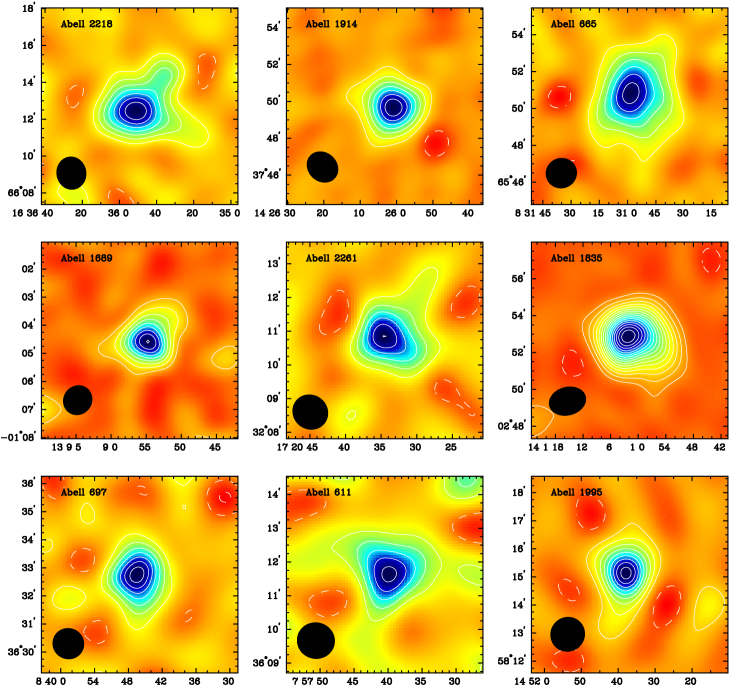
Figure 1: The CLEANed images of the clusters in the sample are presented in order of increasing redshift. The images are plotted with 1.5 $\sigma$ contours, and the restoring beam is shown in the bottom left corner of each image.

The 18 clusters in our sample are listed in Table Galaxy Cluster Gas Mass Fractions from Sunyaev-Zel’dovich Effect Measurements: Constraints on $\Omega_{M}$, along with the published redshifts and $T_{e}$ we used in the $f_{g}$ analysis, and the X-ray luminosities. SZ images of the clusters are presented in Figure 1, ordered by redshift. We note that the quality of the detection reflects the $r.m.s.$ sensitivity of the observation and the intrinsic strength of the SZ effect and not the cluster’s distance. A Gaussian taper is applied to the $u-v$ data to emphasize the structure on large scales. This taper depends on the range of $u$-$v$ radii in each cluster’s data set; the tapers are generally 0.9 to 1.2 k$\lambda$. Higher resolution images can be made from these data in order to emphasize smaller cluster structures,e.g., Carlstrom et al. (1996). Because the primary beam for the BIMA system is considerably larger than that for the OVRO system (396^′′ and 252^′′, respectively), the images produced from BIMA data include information on the decrement at larger scales. The images are plotted in contours of 1.5 $\sigma$, and the restoring beam is shown in the bottom left corner of each image.

The interferometric SZ data is necessarily spatially filtered; the visibility function will not be measured at every spatial frequency. The images are used to indicate the signal-to-noise ratio of the cluster detections, but we do not fit models to the images.

3 SZ Gas Mass and Gas Mass Fraction Measurement Methods

3.1 Model

We compare a model to the data in the spatial frequency domain, where the noise characteristics and the spatial filtering of the interferometer are well-understood.

We fit to a $\beta$-model (Cavaliere & Fusco-Femiano 1976, 1978), which has been widely used to fit the density and temperature profiles of cluster galaxies and the ICM. We make the simplifying assumptions that the cluster gas is isothermal and the density distribution is spherically symmetric. We consider the effects of these simplifications on our results in Section 3.5.

In this model, the electron number density as a function of radius, $r$, takes the form:

$$n_{e}(r)=n_{e\circ}\left(1+{r^{2}\over r_{c}^{2}}\right)^{-3\beta/2},$$ (4)

where $r_{c}$, the core radius, and $\beta$ are fit parameters, and $n_{e\circ}$ is the central electron number density. For isothermal gas with temperature $T_{e}$, Equation 4 predicts the following two-dimensional SZ temperature decrement:

$${\Delta T}\left(\theta\right)=\Delta T(0)\left(1+{\theta^{2}\over\theta_{c}^{2}}\right)^{{1\over 2}-{3\beta\over 2}},$$ (5)

where $\theta=r/D_{A}$, $D_{A}$ is the angular diameter distance, $\theta_{c}=r_{c}/D_{A}$, and $\Delta T(0)$ is the temperature decrement at zero projected radius. The central electron density can therefore be recovered from this relation:

$$n_{e\circ}={-\Delta T(0)\over T_{CMB}}{m_{e}c^{2}\over 2k\sigma_{T}}{1\over T_{e}}\left(D_{A}\int\limits_{-\infty}^{+\infty}\left(1+\left({\theta\over\theta_{c}}\right)^{2}\right)^{-3\beta/2}d\theta\right)^{-1}$$ (6)

where the integral, $dl$, is along the line of sight. The mean molecular weight is assumed to be constant througout the gas, so the electron number density, $n_{e}$, should trace the gas density.

3.2 Fitting Procedure

The change in spectral intensity of the CMB due to the Sunyaev-Zel’dovich effect is calculated for the Rayleigh-Jeans approximation (c.f. Rephaeli (1995); Challinor & Lasenby (1998)):

$${\left.{\Delta T_{SZ}\over T_{CMB}}\right|_{RJ}={yx^{2}e^{x}\over(e^{x}-1)^{2}}[xcoth(x/2)-4+\theta_{e}f(x)],}$$ (7)

where $x=h\nu/kT_{CMB}$ and $\theta_{e}=kT_{e}/m_{e}c^{2}$. We adopt the COBE FIRAS value of $T_{CMB}=2.728$ K (Fixsen et al. 1996). The last term, $\theta_{e}f(x)$, corrects for relativistic effects. At 28.5 GHz, $\Delta T_{SZ}/T_{CMB}=-1.92\ y$ in the non-relativistic Rayleigh-Jeans approximation. Including the relativistic correction for a temperature typical of massive clusters, $kT_{e}=7$ keV, $\Delta T_{SZ}/T_{CMB}=-1.88\ y$.

The data are components of the Fourier transform of the sky brightness distribution, i.e., a measured amplitude and phase for each two-dimensional spatial frequency, or $u$-$v$ pair, sampled. The model is constructed in image space by filling out a regular grid with the SZ model (Equation 5) multiplied by the primary beam. This SZ image is fast Fourier transformed and the model is interpolated to the $u$-$v$ data points to compare with the data using the $\chi^{2}$ statistic. The cluster center, $\beta$, $\theta_{c}$, and $\Delta T(0)$ are allowed to float to find the minimum $\chi^{2}$ using a downhill simplex (Press et al. 1992). The position and flux density of any radio-bright point sources are also fitted. Since the primary beam attenuation at any given point differs between the OVRO and BIMA datasets, and the intrinsic point source flux can vary with time, the point source fluxes for each dataset are allowed to vary individually.

The fits are performed jointly on all datasets for a given cluster. The shortest telescope spacing corresponds to the shadowing limit; for OVRO data this limit is $1\ k\lambda$, for BIMA data this is $0.58\ k\lambda$. We use the holographically determined primary beam models when modeling the data, and the entire datasets are used to do the analysis.

3.3 Constraints on Fit Parameters

The cluster’s centroid position and the point source fluxes and positions are well constrained by the data. The fitting program consistently obtains the same values for the centroid positions. The initial guesses for the point source parameters are made using DIFMAP (Pearson et al. (1994)), an interactive mapping program, to inspect the high spatial frequency ($|u^{2}+v^{2}|>2.0$ k$\lambda$) data in which the SZ effect contributes very little signal. The uncertainty introduced by point sources into the ICM parameters is discussed in Section 3.5.2.

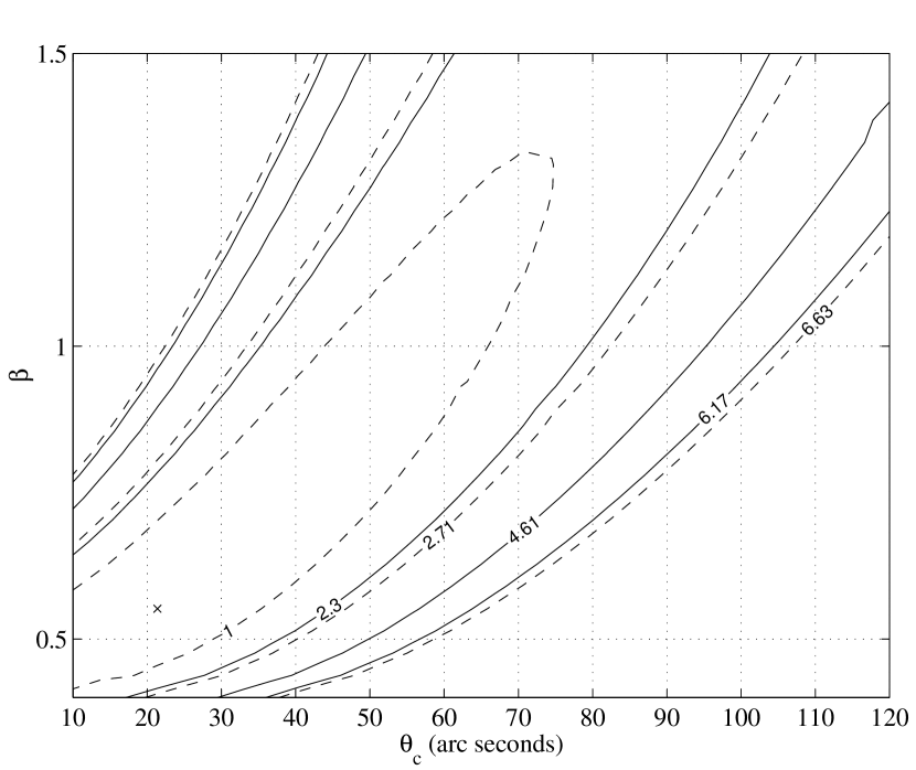
Figure 2: Confidence intervals for $\beta$ and $\theta_{c}$ from a $\beta$-model fit to the Abell 1995 data. At each point in the plot, the central decrement was allowed to assume its best fit value. The solid contours are marked for $\Delta\chi^{2}$ = 2.3, 4.61, and 6.17 which indicate 68.3%, 90.0%, and 95.4% confidence, respectively, for the two-parameter fit. The dashed lines indicate $\Delta\chi^{2}$ =1.0, 2.71, and 6.63. The projection onto the $\beta$ or $\theta_{c}$ axis of the interval contained by these contours indicate the 68.3%, 90% and 99% confidence interval on the single parameter.

The cluster centroid and point source fluxes and positions are fixed to their best-fit values while the cluster shape parameters are fitted. We found no appreciable variation of best fit centroid position with shape parameters. To illustrate the constraints these data place on $\beta$ and $\theta_{c}$  a grid search is performed over these parameters with $\Delta T(0)$ allowed to assume its best fit value at each grid point. In Figure 2, we show the confidence intervals for $\beta$ and $\theta_{c}$ for a representative cluster, Abell 1995. The solid contours indicate $\Delta\chi^{2}$  = 2.3, 4.61, and 6.17 which enclose regions corresponding to 68.3%, 90.0%, and 95.4% confidence, respectively, for the two-parameter fit. The projection of the dashed lines, $\Delta\chi^{2}$ $=1.0$, 2.71, and 6.63, indicate the 68.3%, 90% and 99% confidence interval on the single parameter. At each ($\beta$, $\theta_{c}$) point, the width of the 68% confidence interval for $\Delta T(0)$ is about 10-15% of the best fit $\Delta T(0)$ value. In Patel et al. (2000), we fit the ROSAT HRI data for this cluster, and find the fit values to be consistent with the SZ effect values.

From the figure it is clear that $\beta$ and $\theta_{c}$ are strongly correlated and the fit parameters $\beta$ and $\theta_{c}$ are not well-constrained individually by the SZ effect data.

3.4 Gas Mass Fraction Measurements

The number of electrons in a given volume can be calculated by integrating Equation 4. To recover the ICM mass, we multiply by the proton mass and the nucleon/electron ratio of 1.16. To extract the central electron density, $n_{e\circ}$, for a given set of model parameters and measured electron temperature, we perform the integral in Equation 6. Formally, this integral extends from the observer along the line of sight through the cluster infinitely; in practice, a cutoff radius of 8-10 cluster core radii is used.

We note that although the fit parameters $\beta$, $\theta_{c}$ and $\Delta T(0)$ are not constrained strongly individually, the combination of these three parameters does constrain the gas mass quite well. This follows from the fact that the SZ effect is, under the isothermal assumption, a direct measure of the gas mass on the scales to which our observations are sensitive. We present gas masses for the 18 clusters in our sample in Table 2. To convert angular sizes to lengths, we have assumed $h=0.7$, $\Omega_{M}$= 0.3, $\Omega_{\Lambda}$=0.7.

The distribution of the cluster’s total mass, mainly comprised of dark matter, can be inferred from the modeled gas pressure distribution, since the temperature of the gas and its spatial distribution are constrained by the cluster’s gravitational potential. We make the assumption that the gas is in hydrostatic equilibrium in this potential and that bulk flows and other non-thermal processes do not contribute significantly to the gas pressure. Under the assumptions of spherical symmetry and isothermal gas, the total mass of a cluster within radius $r$, is

$$M(r)={3kT_{e}\beta\over G\mu m_{p}}{r^{3}\over r_{c}^{2}+r^{2}}$$ (8)

where $\mu m_{p}$ is the mean molecular weight of the gas. To calculate $\mu$, we assume the gas has solar metallicity as measured by Anders & Grevesse (1989) and that $\mu$ is constant throughout the gas. The value of $\mu$ will change 3-4 % depending on the solar metallicity measurements one adopts; the metallicity in clusters is not well known, however, and although an incorrect choice for $\mu$ will introduce a systematic error, it will be much smaller than the statistical errors involved. Note from Equation 8 that the total mass depends only on the shape of the gas distribution, and is independent of the value of the central gas density, and therefore of the uncertainties in $\Delta T(0)$. Using the derived shape parameters, $\beta$, $\theta_{c}$, and the measured gas temperature, we derive the total mass, denoting it the “HSE mass”.

To measure the quantities of interest and their associated uncertainties, we determine an appropriate range $\beta$, $\theta_{c}$, and $\Delta T(0)$ for each cluster with a coarse grid, and then construct a finer grid near the best fit parameter values. The cluster’s gas mass, HSE mass, gas mass fraction, and $\chi^{2}$ statistic are derived at each grid point. The 68% confidence interval on each quantity is determined from the range contained in the $\chi^{2}$(best fit) - $\chi^{2}$ = $\Delta\chi^{2}$$<$ 1.0 volume of the parameter grid. We prefer to measure the masses and mass fractions in the largest volume permitted by our method, since the fair sample assumption is best at large radii. The largest spatial scale on which we can constrain the model depends on the $u$-$v$ points at which we significantly detect signal. To determine this scale, we calculate the statistical uncertainties in the $f_{g}$ measurement due to the shape parameter uncertainties for a number of radii from 10^′′ to 150^′′. We find we best constrain $f_{g}$ when it is calculated within a radius of around 65^′′ (see Grego (1999)). The gas masses and gas mass fractions within a 65^′′ radius along with their associated 68% confidence intervals are presented in Table 2. The gas mass and $f_{g}$ results depend on the assumed cosmology through the angular diameter distance, $D_{A}$. For the gas mass fractions reported, we use $\Omega_{M}=0.3,\Omega_{\Lambda}=0.7$.

The SZ gas mass is inversely proportional to the assumed electron temperature: $M_{gas}{\rm(SZ)}\propto 1/T_{e}$ and the HSE total mass measurement is directly proportional to $T_{e}$: $M_{HSE}\propto T_{e}$. The gas mass fraction then is quite sensitive to temperature: $f_{g}\propto 1/T_{e}^{2}$. The uncertainties from the temperature measurement are of the same order as the statistical uncertainties from the SZ model fitting at the lower redshifts, and dominate the SZ uncertainties for the most distant clusters.

3.5 Systematic Effects

3.5.1 Emission-Weighted Temperature

When available, we have used emission-weighted temperatures which were examined and corrected for the presence of cooling flows. The central surface brightness excess exhibited by many clusters is interpreted as emission from centrally-concentrated dense gas, e.g., Fabian (1994), the cooling time of which is shorter than the Hubble time. Such cooling flows can bias the emission-weighted temperatures lower than the density-weighted or virial temperature of the cluster. Allen & Fabian (1998) find that modeling clusters with a cooling flow spectral component in addition to the thermal component significantly reduces the scatter in the luminosity-temperature relation. We have used these cooling flow-corrected temperatures where available.

The emission-weighted ICM temperatures we have adopted from the literature may also have errors due to contamination from other sources in the field. The ASCA observatory was the source for most of the published ICM temperatures we use in this work. As its half power diameter is $\sim 3^{\prime}$, it is nearly impossible to remove the effects of point sources on spectra of distant clusters obtained with ASCA. Since the measurement is so strongly dependent on an accurate measurement of $T_{e}$, this is likely to be the largest source of systematic uncertainty. Fortunately, many of the clusters in our sample are scheduled to be observed with the Chandra and XMM observatories, which will be better able to distinguish ICM emission from point source emission and toconstrain the ICM temperatures.

3.5.2 Radio Point Sources

We detect radio-bright point sources in about half of the observed clusters. The point sources with fluxes exceeding three times the $r.m.s.$ of the high resolution ($\gtrsim 2000\ \lambda$) maps can be reliably identified from the SZ data. We estimate the maximum effect of undetected point sources by adding an on-center point source to a representative cluster data set and fitting this new data set not accounting for the added point source. We place a 3 $\sigma$ point source at the cluster center where typical $r.m.s.$ sensitivities in the OVRO and BIMA high resolution maps are roughly 61 $\mu$Jy and 163 $\mu$Jy respectively. This point source causes the magnitude of the decrement to be underestimated (and thus the gas mass fraction too) by 15% for OVRO data and 20% for BIMA data. Such a point source at the cluster center is highly unlikely but places limits on the maximum effect from undetected point sources.

3.5.3 Departures from an Isothermal, Spherical ICM

Our assumptions that the intra-cluster medium is isothermal and spherical are at some level approximations. Markevitch et al. (1998) report moderate temperature gradients in a sample of 30 nearby clusters, although in a similar analysis, Irwin et al. (1999) do not find such structure. Neglecting to account for existing temperature gradients in the ICM may systematically affect the gas and HSE masses. If such a gradient is present, the true temperature in the central region may be higher than the emission-weighted temperature we use, and the fitted shape parameters from the isothermal SZ analysis may no longer accurately describe the density distribution. As yet, there are no strong observational constraints on temperature structure in clusters beyond z = 0.1, as there have been no suitable telescope facilities for the task. We anticipate that the Chandra and XMM X-ray observatories will greatly improve this situation.

Our observation scheme provides information on the two-dimensional decrement, and we observe that the clusters are not strictly spherical. For this sample of clusters, we find the mean of the best-fit axis ratios to be 0.89 $\pm$ 0.12. In previous work (Grego et al. (2000); Grego (1999)), we relaxed this assumption and permitted the density distribution to be ellipsoidally symmetric, but the unknown orientation and three-dimensional geometry introduce a large uncertainty in the HSE mass. For a sufficiently large sample chosen without orientation bias, deviations from spherical symmetry will not strongly affect the results. As a point of comparison, the effects of cluster shapes on determinations of the cluster size have been investigated in Sulkanen (1999). He calculates Hubble’s constant in a sample of simulated tri-axial clusters by comparing their predicted SZ and X-ray images. The X-ray flux from the cluster at any point in the sky is proportional to $\int n_{e}^{2}dl$, integrated along the line of sight through the cluster, while the SZ effect is proportional to $\int n_{e}dl$, so the two can be compared to derive the size scale of the cluster; when this size scale is compared to the apparent size on the sky, the cluster’s distance and hence $H_{\circ}$ can be inferred. Sulkanen finds that when the images are fit by an spherical beta model with a core radius equal to the arithmetic mean of the two core radii from an elliptical fit, the recovered $H_{\circ}$ for a sample of 25 clusters is unbiased.

In an ongoing analysis of an ensemble of hydrodynamical cluster simulations, we also find that we do not introduce serious error with these assumptions. These simulated clusters are produced within both low and high $\Omega_{M}$ cosmological models, and the temperature and density structure is appropriate for cluster populations experiencing merging similar to that observed at redshifts z$\leq$ 0.1 (Mohr et al. 1995). We produce mock BIMA observations of simulated clusters at the redshifts z=0.2 and z=0.6. Isothermal, spherical $\beta$-model analyses of these SZE observations produce unbiased estimates of the ICM mass enclosed within the radius $r_{2000}$, which roughly corresponds to the scales measured in this experiment (Mohr et al. 2000). Should temperature and density structure in distant clusters be similar to that in the local sample, it should not be a significant source of systematic uncertainty or bias in our measurements.

3.5.4 Validity of the HSE Approximation and Non-thermal Pressure Support

Our method of measuring the total mass assumes the ICM is in hydrostatic equilibrium in the cluster potential and supported only by thermal pressure. One test of this assumption is to compare the HSE-derived total cluster mass to the total mass derived from gravitational lensing models. Some mass comparisons in the literature (Miralda-Escude & Babul (1995); Loeb & Mao (1994); Wu & Fang (1997)) have suggested that the HSE method may systematically underpredict the cluster’s total mass by a factor of 2-3, compared to a strong gravitational lensing analysis. Suggested explanations for this discrepancy include elongation of the cluster along the line of sight and temperature structure in the ICM, which we discuss in Sections 3.5.3, and non-thermal pressure support of the gas in the cluster core.

Further work has suggested that the details of the analysis can have a significant effect, and may resolve the discrepancy. A weak lensing analysis was performed by Squires et al. (1997) on the cluster Abell 2218, which appears to have discrepant masses in each of the three analyses above. This analysis, at larger radius than the strong lensing analyses, show the two methods predict masses which are consistent within the experimental uncertainties. In an examination of a sample of 13 clusters, Allen & Fabian (1998) finds that the lensing and HSE masses agree for clusters which appear to have a strong central cooling flow, when the cooling flow is taken into account; in these clusters, the X-ray and lensing core radii are consistent with each other, and the mass agreements suggest HSE is a reasonable approximation. For clusters without strong cooling flows, the X-ray core radii are generally larger than the lensing radii, and offsets between the centers of the distributions are observed, suggesting that HSE is not appropriate for the cluster cores. Outside the cluster core (at radii $\geq\sim$ 400 kpc, weak lensing and X-ray masses are consistent with each other both for cooling flow and non-cooling flow clusters. Lewis et al. (1999) compare X-ray HSE masses to the dynamical masses calculated from the galaxy velocity dispersions, and find the average M_dyn/M_HSE to be 1.04$\pm$0.07, which also suggests the HSE method does not introduce a systematic bias.

Possible sources of non-thermal pressure in the ICM are bulk flows and magnetic fields in the gas. Intracluster magnetic fields are typically a few $\mu$G (Kim et al. (1990); Taylor & Perley (1993)), an order of magnitude smaller than the level at which the fields would contribute significantly to the dynamics of cluster gas, although stronger fields, $\sim 10-$100 $\mu$G, have been measured in a few clusters (Taylor & Perley (1993)). There is some evidence for the persistence of bulk flows in clusters undergoing merger events (Bliton et al. (1998)). It remains to further investigation how significant a role these effects play in the physics of cluster gas, but currently there is no evidence to suggest a significant systematic error in the HSE method.

3.5.5 Cosmic Microwave Background Anisotropies

The SZE observations are also sensitive to intrinsic and secondary anisotropy in the Cosmic Microwave Background (CMB) radiation. The theoretical expected and observed level of CMB anisotropy at the angular scales corresponding to those used for the SZE measurements presented here is small and safely ignored. The contribution of primary anisotropy for a window function appropriate for our shortest baselines, for which the contribution would be strongest, has been calculated by Holzapfel et al. (2000a). For a flat universe, as indicated by recent CMB observations (Miller et al. 1999; de Bernardis et al. 2000; Hanany et al. 2000) the $r.m.s.$ temperature fluctuations contributed by primary CMB anisotropy within our maps should be of order $2\mu$K or less.

At the angular scales of our SZE measurements, secondary CMB anisotropy is expected to be stronger than intrinsic anisotropy. Holzapfel et al. (2000a) have tabulated the expected range of the magnitude of the temperature anisotropy due to the Visniac Effect and inhomogenous reionization. The upper range for the $r.m.s.$ temperature fluctuations at angular scales appropriate for the SZE measurements is only 5.6 $\mu$K and 3.9 $\mu$K, respectively. Added in quadrature, this gives an expected upper limit to the $r.m.s.$ temperature fluctuations in our SZE observations of only 6.8 $\mu$K. If present, this signal would contribute to the SZE maps as noise (i.e., would not lead to a bias in our SZE measurements). This level is much smaller than the noise level obtained in our SZE observations.

The dominant contribution to secondary anisotropy at the relevant angular scales is likely to be the SZE from undetected low mass clusters. Holder & Carlstrom (1999) estimate $r.m.s.$ temperature fluctuations of order 2 $\mu$K to 12 $\mu$K for the range of models they consider. Again, this level is small compared to our uncertainties, although approaching the noise level in our deepest fields.

It is unnecessary to depend on theoretical estimates of contributions from CMB anisotropy as we have direct measurements of ‘blank’ fields obtained with the same instrument as for the SZE observations (Holzapfel et al. 2000a). The $r.m.s.$ level obtained on the deepest fields ranges from 16 $\mu$K to 20 $\mu$K, just slightly above that expected from the instrumental noise. The most likely level of anisotropy, including undetected point sources, derived from the blank field data is 12 $\mu$K and the 95% confidence level upper limit is 19 $\mu$K.

We conclude that temperature fluctuations due to primary and secondary CMB anisotropy should have a negligible effect on the results derived from the SZE measurements reported here.

4 Results and Discussion

4.1 Gas Mass Fractions

As we discussed in Section 3.4, we measure the gas mass fraction within a fixed angular radius, which results in the measurements being made at different physical scales for clusters at different distances. To compare the gas mass fractions of different clusters, and to derive a result useful for cosmological tests, we scale the results for each cluster to a fiducial radius. An analytical expression for the variation in $f_{g}$ with radius is suggested by Evrard (1997), based on results in Evrard et al. (1996) and found to be consistent with the $f_{g}$ variation reported in the David et al. (1995) sample. We use a modified version of this to extrapolate the gas mass fractions we measure at 65^′′ to the gas mass fraction expected at $r_{500}$, the radius at which the cluster’s total mass density is 500 times the critical mass density, where the cluster’s baryon fraction should closely reflect the universal value. The physical radius at which the overdensity is 500 depends on the cluster’s temperature (a mass indicator), and also its redshift, since the critical density will change with $z$. The scaling expression is as follows:

$${f_{g}(r_{500}(T_{e}))=f_{g}(r_{X})\left({r_{500}(T_{e})\over r_{X}}\right)^{\eta}},$$ (9)

where $\eta$ = 0.17, $f_{g}(r_{500}(T_{e}))$ is the gas mass fraction within $r_{500}$, and $r_{X}$ is the radius within which the gas mass fraction is measured. We modify Evrard’s expression for $r_{500}$, derived for low redshift clusters, to include the change in the value of $\rho_{c}$ with redshift; $\rho_{c}(z)=\rho_{c}(z=0)(H/H_{\circ})^{2}$, where $H^{2}=H_{\circ}^{2}[(1+z)^{3}\Omega_{M}+(1+z)^{2}(1-\Omega_{M}-\Omega_{\Lambda})+\Omega_{\Lambda}]$ (c.f. Peebles 1993, Eqn. 13.3):

$${r_{500}(T_{e})=(1.24\pm 0.09)\left({T_{e}\over 10\ {\rm keV}(H/H_{\circ})^{2}}\right)^{1/2}h^{-1}{\rm Mpc}}.$$ (10)

The gas mass fractions within $r_{500}$ as derived by this relation are presented in Table 2. Figures 3a. and b. show the gas mass fractions at $r_{500}$ as a function of $T_{e}$ and redshift. We see no correlation of gas mass fraction with temperature. We see no significant evolution of $f_{g}$ with redshift. Since $f_{g}$ depends on the cluster distance, $f_{g}\propto$ D_A, and therefore the chosen cosmology, measurement of the gas mass fraction over a range of redshifts could be used in principle to constrain cosmological models.

We calculate the mean gas mass fraction for the entire cluster sample, and derive the 68% confidence interval from the $\Delta\chi^{2}$ statistic to a constant-value fit. For the entire sample, assuming $\Omega_{M}$=0.3, $\Omega_{\Lambda}$=0.7, we find the mean gas mass fraction to be $0.081^{+0.009}_{-0.011}h^{-1}_{100}$. We also calculate the mean and uncertainty for $f_{g}$ in the full sample, using two alternative cosmologies, ($\Omega_{M}$=0.3, $\Omega_{\Lambda}$=0.0) and ($\Omega_{M}$=1.0, $\Omega_{\Lambda}$=0.0), to calculate the distances and scaling relation. In Table 3, we report these and the associated reduced chi-squared ($\chi^{2}_{red}$) statistics, which range from 1.021 to 1.056 for the full sample fits. The $\chi^{2}_{red}$ values do not differ significantly enough to discriminate between cosmologies, and it is clear that currently the uncertainties are too large for a cosmological test via geometry.

We also calculate the mean $f_{g}$ in a homogeneous subsample of five clusters. These clusters are the five most luminous clusters in the flux-limited EMSS cluster sample with $z>0.26$ and declination $>-10^{\circ}$: MS0451.6-0305, MS1137.5+6625, CL0016+16, MS1358.4+6245, & MS1054.4-0321. For our standard cosmology, we find the mean in this sample to be $0.089^{+0.018}_{-0.019}h^{-1}_{100}$. In all three cosmologies, the gas mass fraction in the homogenous sample is consistent with the full sample value.

We compare these SZ-derived gas mass fractions to other SZ-derived $f_{g}$ measurements. Recent cluster gas mass fraction measurements from SZ effect observations are presented in Myers et al. (1997). In this work, the integrated SZ effect is measured using a single radio dish operating at centimeter wavelengths. The integrated SZ effect is used to normalize a model for the gas density from published X-ray analyses, and this gas mass is compared to the published total masses to determine the gas mass fraction. For three nearby clusters, A2142, A2256 and the Coma cluster, Myers et al. (1997) find a gas mass fraction of $(0.061\pm 0.011)h_{100}^{-1}$ at radii of 1-1.5 $h_{100}^{-1}$ Mpc; for the cluster Abell 478, they report a gas mass fraction of $(0.16\pm 0.014)h_{100}^{-1}$.

4.2 Comparison of SZ and X-ray Results

Gas mass fractions derived from X-ray images for a large, homogeneous, nearby sample of clusters are presented in Mohr et al. (1999). For a subsample of 28 clusters with $T_{e}>5$ keV, they find the mean gas mass fraction within $r_{500}$ to be $(0.0749\pm 0.0021)h_{100}^{-3/2}$ at 90% confidence. The gas mass fractions derived from SZ measurements depend differently on the cosmology assumed than those derived from X-ray images, and this should be noted when comparing the results.

Qualitatively, though, the comparison does not suggest any large systematic offsets. This is a significant result, because a large clumping factor, $c=<n_{e}^{2}>^{1/2}/<n_{e}>$, has been suggested as an explanation for the high gas mass fractions in clusters (White et al. 1993; Evrard 1997). A cluster with clumping factor $c$ would only require 1/$c$ as much gas mass to produce the observed emission, and so the SZ and X-ray gas mass fraction measurements would differ by a factor of $\sim c$.

4.3 Comparison of Baryon Fraction with $\Omega_{B}$

The relative abundance of deuterium and hydrogen provides a particularly strong constraint on the baryonic matter density (Copi et al. 1995). A firm upper limit to $\Omega_{B}$ is set by the presence of deuterium in the local interstellar medium. This constrains the value of $\Omega_{B}$ to be less than $0.031h_{100}^{-2}$ (Linsky et al. 1995). Measurements of the D/H ratio in metal-poor Lyman-$\alpha$ absorption line systems in high-redshift quasars put an even more stringent constraint on the baryonic mass density. For this analysis, we adopt the published value at 95% confidence from the Burles & Tytler (1998) absorption line anaylsis, $\Omega_{B}=(0.019\pm 0.002)h_{100}^{-2}$.

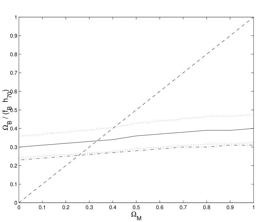
Figure 4: Upper limit on the total matter density, $\Omega_{M}$$\leq\Omega_{B}/(f_{B}h_{70})$ (full line) and its associated 68% confidence region (dotted lines), as a function of cosmology ($\Omega_{\Lambda}$$\equiv$ 1 - $\Omega_{M}$). The baryon fraction is a function of cosmology through the angular diameter distance relation as well as the scaling relation in Equation 9. The intercept between the upper dotted line and the dashed line [$\Omega_{M}$= $\Omega_{B}/(f_{B}h_{70})]$ gives the upper limit to $\Omega_{M}$ at 68% confidence. The dot-dashed line shows the total matter density when the baryon fraction includes an estimate of the contribution from baryons in galaxies and those lost during cluster formation. The intercept of the dot-dashed line and the dashed line gives our best estimate of $\Omega_{M}$ ($\sim$0.25) assuming a flat universe with $h$=0.7.

We can use the gas mass fractions to find the value of $\Omega_{M}$ in a self-consistent manner. In Figure 4, we show the value of $\Omega_{M}$ implied by the measured gas mass fractions when we assume a flat universe ($\Omega_{\Lambda}$$\equiv$ 1- $\Omega_{M}$) and $h=0.7$ to calcluate the angular diameter distance and $r_{500}$ scaling factor from Equation 9: $\Omega_{M}$ $\leq\Omega_{B}/f_{B}/h_{70}$ . The upper limit to $\Omega_{M}$ and its associated 68% confidence interval is shown as a function of $\Omega_{M}$. The measured gas mass fractions are consistent with a flat universe and $h=0.7$ when $\Omega_{M}$ is less than 0.40, at 68% confidence. For our measurements to be consistent with $\Omega_{M}$ = 1.0 in a flat universe, the Hubble constant must be very low, $h$ less than $\sim$ 0.30.

For a more realistic estimate, we could include the baryon contribution from galaxies, and attempt to account for the overall dimunition of the baryon fraction in clusters with respect to the universal value, since some baryons are expected to not become bound to the cluster. Following White et al. (1993), we estimate the galaxy mass to be a fixed fraction of the cluster gas, with the same fraction as is observed in the Coma cluster, $M_{B}=M_{gas}(1+0.20h^{3/2})$. For a realistic equation of state, the gas in the cluster will be more extended than the dark matter and the baryon fraction at $r_{500}$ will be a modest underestimate of the true baryon fraction (Evrard 1997), $f_{g}(r_{500})=0.85\times f_{b}({\rm universal})$. These assumptions lead to

$$f_{B}=(f_{g}(1+0.2h^{3/2})/0.85).$$ (11)

Using this estimate of the baryon fraction, and $h=0.7$ in a flat cosmology, in Figure 4 we show our best estimate of $\Omega_{M}$ as a function of cosmology. Thus we find our best estimate of $\Omega_{M}$ is $\sim$0.25.

4.4 Future Work

There are several improvements to this work which will be made in the near future. More clusters will be added to the sample as SZ observations continue. And the potential also exists for improving the centimeter-wave SZ interferometer system dramatically by taking advantage of the 10 GHz output of the SZ receivers; currently a maximum of 2 GHz are correlated at OVRO and effective bandwidth of 0.5 GHz are correlated at BIMA.

One of the main sources of uncertainty in these measurements originates in the emission-weighted gas temperature measurements; as $f_{g}\propto T_{e}^{-2}$, the 10-20% uncertainties in $T_{e}$ roughly double to 20-40% uncertainties in the gas mass fraction. A large number of these clusters are scheduled to be observed in the Chandra X-Ray Observatory GTO and GO phases, which should improve the situation considerably.

Numerical simulations will also help identify other sources of systematic error incurred in the observational and analysis program. An analysis is in preparation of hydrodynamic simulations of a sample of clusters to quantify any biases we may introduce to the gas mass fraction measurements with the interferometric method and through the assumptions we make in the fitting and analysis of the clusters.

Many thanks are due to the staff at the BIMA and OVRO observatories for their contributions to this project, especially Rick Forster, John Lugten, Steve Padin, Dick Plambeck, Steve Scott, and Dave Woody. Many thanks to Cheryl Alexander for her work on the system hardware. This work is supported by NASA LTSA grant NAG5-7986. LG, EDR, and SKP gratefully thank the NASA GSRP program for its support. JJM is supported by Chandra Fellowship grant PF8-1003, awarded through the Chandra Science Center. The Chandra Science Center is operated by the Smithsonian Astrophysical Observatory for NASA under contract NAS8-39073. Radio astronomy with the OVRO and BIMA millimeter arrays is supported by NSF grants AST 96-13717 and AST 96-19938, respectively. The funds for the additional hardware for the SZ experiment were from a NASA CDDF grant, a NSF-YI Award, and the David and Lucile Packard Foundation.

Table 1: The Cluster Sample

Cluster	z	reference	$T_{e}$	reference	$L_{x}$	band	reference
			(keV)		($10^{45}$ erg/s)	(keV)
Abell 2218	0.171	LB	7.05${}^{+0.36}_{-0.35}$	AF	1.08	2-10	AF
Abell 1914	0.1712	BA	10.7${}^{+1.5}_{-1.5}$	EB	1.8	0.3-3.5	EB
Abell 665	0.1818	SR	9.03${}^{+0.58}_{-0.52}$	AF	1.78	2-10	AF
Abell 1689	0.1832	SR	10.0 ${}^{+1.2}_{-0.80}$	AF	3.24	2-10	AF
Abell 2261	0.224	C95	10.09 ${}^{+5.9}_{-2.2}$	AF	2.39	2-10	AF
Abell 1835	0.2528	A92	9.8 ${}^{+2.3}_{-1.3}$	AF	4.54	2-10	AF
Abell 697	0.282	C95	9.80 ${}^{+0.70}_{-0.70}$	AF	1.574	0.1-2.4	E98
Abell 611	0.288	C95	6.60 ${}^{+0.60}_{-0.60}$	AF	1.04	0.1-2.4	E98
Abell 1995	0.3219	PA	8.59${}^{+0.86}_{-0.67}$	MS	0.87	0.3-3.5	MS
ZwCl 1953	0.32	BA	13.2${}^{+2.0}_{-2.0}$	E98	2.86	0.3-3.5	E98
MS1358.4+6245	0.328	GI	7.48 ${}^{+0.83}_{-0.70}$	AF	1.08	2-10	AF
RXJ 1532.9+3021	0.345	EB	12.20${}^{+2.00}_{-2.00}$	E98	2.374	0.3-3.5	E98
Abell 370	0.374	M88	6.60 ${}^{+1.10}_{-0.90}$	OT	1.3	2-10	AE
CL0016+16	0.5479	GI	7.55${}^{+0.72}_{-0.58}$	HB	1.46	0.3-3.5	GI
MS0451.6-0305	0.55	GI	10.17${}^{+1.55}_{-1.26}$	MS	0.7	0.3-3.5	GI
MS2053.7-0449	0.583	GI	6.60 ${}^{+2.00}_{-2.00}$	AEest	0.58	0.3-3.5	GI
MS1137.5+6625	0.78	GI	5.70 ${}^{+2.10}_{-1.10}$	D99	1.9	0.3-3.5	GI
MS1054.5-0321	0.826	LG	12.30${}^{+3.10}_{-2.20}$	D98	9.3	0.3-3.5	LG

References. — A92 Allen (1992); AF Allen & Fabian (1998); AE Arnaud & Evrard (1998); AEest estimated from $L_{x}$-T relation of AE; BA Bade, N. et al. (1998); C95 Crawford et al. (1995); D98 Donahue et al. (1998); D99 Donahue et al. (1999); EB Ebeling et al. (1996), E98 Ebeling (1998); GI Gioia et al. (1990); HB Hughes & Birkinshaw (1998); LB LeBorgne et al. (1992); LG Luppino & Gioia (1995); M88 Mellier et al. (1988); MS Mushotzky & Scharf (1997); OT Ota et al. (1998); PA Patel et al. (2000); SR Struble & Roo d (1991)

Table 2: SZ-derived Gas Masses and Mass Fractions, using $\Omega_{M}=0.3$, $\Omega_{\Lambda}=0.7$

Cluster	gas mass within 65′′	$f_{g}h$ (within 65${}^{\prime\prime})$	$\underline{f_{g}(r_{500})}$	$f_{g}h$ (within $r_{500})$
	($h^{2}/10^{12}M_{\circ}$)		$f_{g}(65^{\prime\prime})$
Abell 2218	4.91 ${}^{+1.39}_{-1.76}$	0.179${}^{+0.037}_{-0.046}$	1.40	0.250${}^{+0.051}_{-0.065}$
Abell 1914	3.51 ${}^{+1.04}_{-1.05}$	0.037${}^{+0.019}_{-0.019}$	1.45	0.053${}^{+0.027}_{-0.027}$
Abell 665	1.97 ${}^{+0.67}_{-0.54}$	0.042${}^{+0.022}_{-0.022}$	1.42	0.060${}^{+0.031}_{-0.031}$
Abell 1689	4.60 ${}^{+0.82}_{-1.14}$	0.068${}^{+0.020}_{-0.023}$	1.43	0.098${}^{+0.029}_{-0.033}$
Abell 2261	3.12 ${}^{+2.74}_{-3.76}$	0.027${}^{+0.070}_{-0.016}$	1.39	0.037${}^{+0.097}_{-0.022}$
Abell 1835	4.82 ${}^{+1.33}_{-2.31}$	0.085${}^{+0.026}_{-0.042}$	1.36	0.116${}^{+0.035}_{-0.057}$
Abell 697	3.66 ${}^{+2.01}_{-0.71}$	0.021${}^{+0.043}_{-0.006}$	1.34	0.029${}^{+0.057}_{-0.009}$
Abell 611	5.05 ${}^{+4.11}_{-1.37}$	0.048${}^{+0.140}_{-0.024}$	1.29	0.062${}^{+0.180}_{-0.030}$
ZwCl 1953	3.23 ${}^{+1.81}_{-1.43}$	0.054${}^{+0.019}_{-0.027}$	1.34	0.073${}^{+0.026}_{-0.036}$
Abell 1995	7.44 ${}^{+1.69}_{-1.92}$	0.079${}^{+0.030}_{-0.031}$	1.30	0.102${}^{+0.039}_{-0.041}$
MS1358.4+6245	6.00 ${}^{+1.59}_{-2.17}$	0.097${}^{+0.067}_{-0.049}$	1.28	0.124${}^{+0.086}_{-0.062}$
RXJ 1532.9+3021	4.80 ${}^{+1.85}_{-1.71}$	0.038${}^{+0.030}_{-0.016}$	1.32	0.050${}^{+0.040}_{-0.021}$
Abell 370	8.57 ${}^{+2.60}_{-2.90}$	0.087${}^{+0.045}_{-0.048}$	1.24	0.108${}^{+0.055}_{-0.059}$
CL0016+16	18.85${}^{+4.64}_{-4.11}$	0.139${}^{+0.086}_{-0.039}$	1.19	0.165${}^{+0.103}_{-0.046}$
MS0451.6-0305	21.13${}^{+5.62}_{-7.98}$	0.128${}^{+0.050}_{-0.055}$	1.22	0.155${}^{+0.061}_{-0.068}$
MS2053.7-0449	6.44 ${}^{+7.21}_{-4.19}$	0.044${}^{+0.136}_{-0.034}$	1.16	0.052${}^{+0.158}_{-0.040}$
MS1137.5+6625	15.75${}^{+6.33}_{-11.74}$	0.062${}^{+0.037}_{-0.048}$	1.10	0.068${}^{+0.041}_{-0.053}$
MS1054.5-0321	14.18${}^{+5.27}_{-7.28}$	0.045${}^{+0.024}_{-0.024}$	1.17	0.053${}^{+0.028}_{-0.028}$

Table 3: Mean Gas Mass Fractions

		$\Omega_{M}$=0.3,$\Omega_{\Lambda}$=0.7		$\Omega_{M}$=0.3,$\Omega_{\Lambda}$=0.0		$\Omega_{M}$=1.0,$\Omega_{\Lambda}$=0.0
sample	number of clusters	$\overline{f_{g}h_{100}}$	$\chi^{2}_{red}$	$\overline{f_{g}h_{100}}$	$\chi^{2}_{red}$	$\overline{f_{g}h_{100}}$	$\chi^{2}_{red}$
full sample	18	$0.081^{+0.009}_{-0.011}$	1.021	$0.074^{+0.008}_{-0.009}$	1.027	$0.068^{+0.009}_{-0.008}$	1.056
EMSS subsample	6	$0.089^{+0.018}_{-0.019}$	1.208	$0.077^{+0.017}_{-0.016}$	1.258	$0.067^{+0.015}_{-0.014}$	1.352

Note. — The mean gas mass fractions for the noted samples are presented. The gas mass fractions depend on $D_{A}^{-1}$ and so the results are presented for three sets of cosmological parameters. ($H_{\circ}=100h$ km s^-1 Mpc^-1).

Figure 3: Gas mass fractions within $r_{500}$ for the entire sample, assuming the cosmology ($\Omega_{M}$=0.3, $\Omega_{\Lambda}$=0.7). a) Gas mass fraction vs. ICM emission-weighted temperature. b) Gas mass fraction versus redshift.

References

- Allen & Fabian (1998) Allen, S. W. & Fabian, A. C. 1998, MNRAS, 297, L57
- Anders & Grevesse (1989) Anders, E. & Grevesse, N. 1989, Geochim. Cosmochim. Acta, 53, 197
- Bliton et al. (1998) Bliton, M., Rizza, E., Burns, J. O., Owen, F. N., & Ledlow, M. J. 1998, MNRAS, 301, 609
- Burles & Tytler (1998) Burles, S. & Tytler, D. 1998, ApJ, 499, 699+
- Carlstrom et al. (1996) Carlstrom, J. E., Joy, M., & Grego, L. 1996, ApJ, 456, L75
- Carlstrom et al. (2000) Carlstrom, J. E., Joy, M. K., Grego, L., Holder, G. P., Holzapfel, W. L., Mohr, J. J., Patel, S., & Reese, E. D. 2000, Physica Scripta Volume T, 85, 148
- Cavaliere & Fusco-Femiano (1976) Cavaliere, A. & Fusco-Femiano, R. 1976, A&A, 49, 137
- Cavaliere & Fusco-Femiano (1978) —. 1978, A&A, 70, 677
- Challinor & Lasenby (1998) Challinor, A. & Lasenby, A. 1998, ApJ, 499, 1
- Copi et al. (1995) Copi, C. J., Schramm, D. N., & Turner, M. S. 1995, Science, 267, 192+
- David et al. (1995) David, L. P., Jones, C., & Forman, W. 1995, ApJ, 445, 578
- de Bernardis et al. (2000) de Bernardis, P., Ade, P. A. R., Bock, J. J., Bond, J. R., Borrill, J., Boscaleri, A., Coble, K., Crill, B. P., De Gasperis, G., Farese, P. C., Ferreira, P. G., Ganga, K., Giacometti, M., Hivon, E., Hristov, V. V., Iacoangeli, A., Jaffe, A. H., Lange, A. E., Martinis, L., Masi, S., Mason, P. V., Mauskopf, P. D., Melchiorri, A., Miglio, L., Montroy, T., Netterfield, C. B., Pascale, E., Piacentini, F., Pogosyan, D., Prunet, S., Rao, S., Romeo, G., Ruhl, J. E., Scaramuzzi, F., Sforna, D., & Vittorio, N. 2000, Nature, 404, 955
- Ebeling et al. (1998) Ebeling, H., Edge, A. C., Bohringer, H., Allen, S. W., Crawford, C. S., Fabian, A. C., Voges, W., & Huchra, J. P. 1998, MNRAS, 301, 881
- Ebeling et al. (1996) Ebeling, H., Voges, W., Bohringer, H., Edge, A. C., Huchra, J. P., & Briel, U. G. 1996, MNRAS, 281, 799
- Evrard (1997) Evrard, A. E. 1997, MNRAS, 292, 289+
- Evrard et al. (1996) Evrard, A. E., Metzler, C. A., & Navarro, J. F. 1996, ApJ, 469, 494+
- Fabian (1994) Fabian, A. C. 1994, ARA&A, 32, 277
- Fixsen et al. (1996) Fixsen, D. J., Cheng, E. S., Gales, J. M., Mather, J. C., Shafer, R. A., & Wright, E. L. 1996, ApJ, 473, 576
- Forman & Jones (1982) Forman, W. & Jones, C. 1982, ARA&A, 20, 547
- Gioia & Luppino (1994) Gioia, I. M. & Luppino, G. A. 1994, ApJS, 94, 583
- Gioia et al. (1990) Gioia, I. M., Maccacaro, T., Schild, R. E., Wolter, A., Stocke, J. T., Morris, S. L., & Henry, J. P. 1990, ApJS, 72, 567
- Goldin et al. (1997) Goldin, A. B., Kowitt, M. S., Cheng, E. S., Cottingham, D. A., Fixsen, D. J., Inman, C. A., Meyer, S. S., Puchalla, J. L., Ruhl, J. E., & Silverberg, R. F. 1997, ApJ, 488, L161
- Grego (1999) Grego, L. 1999, PhD thesis, Caltech
- Grego et al. (2000) Grego, L., Carlstrom, J. E., Joy, M. K., Reese, E. D., Holder, G. P., Patel, S., Cooray, A. R., & Holzapfel, W. L. 2000, ApJ, 539, 39
- Hanany et al. (2000) Hanany, S., Ade, P., Balbi, A., Bock, J., Borrill, J., Boscaleri, A., de Bernardis, P., Ferreira, P. G., Hristov, V. V., Jaffe, A. H., Lange, A. E., Lee, A. T., Mauskopf, P. D., Netterfield, C. B., Oh, S., Pascale, E., Rabii, B., Richards, P. L., Smoot, G. F., Stompor, R., Winant, C. D., & Wu, J. H. P. 2000, ApJ, submitted, astro-ph/0005123
- Holder & Carlstrom (1999) Holder, G. & Carlstrom, J. 1999, in Microwave Foregrounds, ed. A. de Oliveira-Costa & M. Tegmark (San Francisco: ASP– astro-ph/9904220)
- Holzapfel et al. (2000a) Holzapfel, W. L., Carlstrom, J. E., Grego, L., Holder, G., Joy, M., & Reese, E. D. 2000a, ApJ, 539, 57
- Holzapfel et al. (2000b) Holzapfel, W. L., Carlstrom, J. E., Grego, L., Joy, M., & Reese, E. D. 2000b, ApJ, 539, 67
- Hu et al. (1997) Hu, W., Sugiyama, N., & Silk, J. 1997, Nature, 37, astro-ph/9604166
- Irwin et al. (1999) Irwin, J. A., Bregman, J. N., & Evrard, A. E. 1999, ApJ, 519, 518
- Kim et al. (1990) Kim, K. ., Kronberg, P. P., Dewdney, P. E., & Landecker, T. L. 1990, ApJ, 355, 29
- Lewis et al. (1999) Lewis, A. D., Ellingson, E., Morris, S. L., & Carlberg, R. G. 1999, ApJ, 517, 587
- Linsky et al. (1995) Linsky, J. L., Diplas, A., Wood, B. E., Brown, A., Ayres, T. R., & Savage, B. D. 1995, ApJ, 451, 335+
- Loeb & Mao (1994) Loeb, A. & Mao, S. 1994, ApJ, 435, L109
- Markevitch et al. (1998) Markevitch, M., Forman, W. R., Sarazin, C. L., & Vikhlinin, A. 1998, ApJ, 503, 77
- Mason et al. (1999) Mason, B. S., Leitch, E. M., Myers, S. T., Cartwright, J. K., & Readhead, A. C. S. 1999, AJ, 118, 2908
- Miller et al. (1999) Miller, A. D., Caldwell, R., Devlin, M. J., Dorwart, W. B., Herbig, T., Nolta, M. R., Page, L. A., Puchalla, J., Torbet, E., & Tran, H. T. 1999, ApJ, 524, L1
- Miralda-Escude & Babul (1995) Miralda-Escude, J. & Babul, A. 1995, ApJ, 449, 18+
- Mohr et al. (1995) Mohr, J. J., Evrard, A. E., Fabricant, D. G., & Geller, M. J. 1995, ApJ, 447, 8
- Mohr et al. (1999) Mohr, J. J., Mathiesen, B., & Evrard, A. E. 1999, ApJ, 517, 627
- Mohr et al. (2000) Mohr, J. J., Reese, E. D., Ellingson, E., Lewis, A. D., & Evrard, A. E. 2000, ApJ, in press
- Myers et al. (1997) Myers, S. T., Baker, J. E., Readhead, A. C. S., Leitch, E. M., & Herbig, T. 1997, ApJ, 485, 1
- Neumann & Böhringer (1997) Neumann, D. M. & Böhringer, H. 1997, MNRAS, 289, 123
- Nichol et al. (1997) Nichol, R. C., Holden, B. P., Romer, A. K., Ulmer, M. P., Burke, D. J., & Collins, C. A. 1997, ApJ, 481, 644+
- Padin et al. (1991) Padin, S., Scott, S. L., Woody, D. P., Scoville, N. Z., Seling, T. V., Finch, R. P., Giovanine, C. J., & Lawrence, R. P. 1991, PASP, 103, 461
- Patel et al. (2000) Patel, S. K., Joy, M., Carlstrom, J. E., Holder, G. P., Reese, E. D., Gomez, P. L., Hughes, J. P., Grego, L., & Holzapfel, W. L. 2000, ApJ–submitted
- Pearson et al. (1994) Pearson, T. J., Shepherd, M. C., Taylor, G. B., & Myers, S. T. 1994, BAAS, 185, 0808
- Peres et al. (1998) Peres, C. B., Fabian, A. C., Edge, A. C., Allen, S. W., Johnstone, R. M., & White, D. A. 1998, MNRAS, 298, 416
- Ponman et al. (1996) Ponman, T. J., Bourner, P. D. J., Ebeling, H., & Bohringer, H. 1996, MNRAS, 283, 690
- Reese et al. (2000) Reese, E. D., Mohr, J. J., Carlstrom, J. E., Joy, M., Grego, L., Holder, G. P., Holzapfel, W. L., Hughes, J. P., Patel, S. K., & Donahue, M. 2000, ApJ, 533, 38
- Rephaeli (1995) Rephaeli, Y. 1995, ApJ, 445, 33
- Rudy (1987) Rudy, D. J. 1987, PhD thesis, California Inst. of Tech., Pasadena.
- Scoville et al. (1993) Scoville, N. Z., Carlstrom, J. E., Chandler, C. J., Phillips, J. A., Scott, S. L., Tilanus, R. P. J., & Wang, Z. 1993, PASP, 105, 1482
- Squires et al. (1997) Squires, G., Neumann, D. M., Kaiser, N., Arnaud, M., Babul, A., Boehringer, H., Fahlman, G., & Woods, D. 1997, ApJ, 482, 648+
- Stocke et al. (1991) Stocke, J. T., Morris, S. L., Gioia, I. M., Maccacaro, T., Schild, R., Wolter, A., Fleming, T. A., & Henry, J. P. 1991, ApJS, 76, 813
- Sulkanen (1999) Sulkanen, M. E. 1999, ApJ, 522, 59
- Sunyaev & Zel’dovich (1972) Sunyaev, R. A. & Zel’dovich, Y. B. 1972, Comments Astrophys. Space Phys., 4, 173
- Taylor & Perley (1993) Taylor, G. B. & Perley, R. A. 1993, ApJ, 416, 554+
- Wagoner et al. (1967) Wagoner, R. V., Fowler, W. A., & Hoyle, F. 1967, ApJ, 148, 3+
- Welch et al. (1996) Welch, W. J., Thornton, D. D., Plambeck, R. L., Wright, M. C. H., Lugten, J., Urry, L., Fleming, M., Hoffman, W., Hudson, J., Lum, W. T., Forster, J. . R., Thatte, N., Zhang, X., Zivanovic, S., Snyder, L., Crutcher, R., Lo, K. Y., Wakker, B., Stupar, M., Sault, R., Miao, Y., Rao, R., Wan, K., Dickel, H., Blitz, L., Vogel, S. N., Mundy, L., Erickson, W., Teuben, P. J., Morgan, J., Helfer, T., Looney, L., de Gues, E., Grossman, A., Howe, J. E., Pound, M., & Regan, R. 1996, PASP, 108, 93+
- White & Fabian (1995) White, D. A. & Fabian, A. C. 1995, MNRAS, 273, 72
- White et al. (1994) White, M., Scott, D., & Silk, J. 1994, ARA&A, 32, 319
- White et al. (1993) White, S. D. M., Navarro, J. F., Evrard, A. E., & Frenk, C. S. 1993, Nature, 366, 429+
- Wu & Fang (1997) Wu, X. & Fang, L. 1997, ApJ, 483, 62+