Near-infrared spectroscopy of the circumnuclear star formation regions in M100: Evidence for sequential triggering

Abstract

We present low resolution ($R\sim 450$) $K$-band spectroscopy for 16 of the 43 circumnuclear star-forming knots in M100 identified by Ryder & Knapen (1999). We compare our measurements of equivalent widths for the Br$\gamma$ emission line and CO 2.29 $\mu$m absorption band in each knot with the predictions of starburst models from the literature, and derive ages and burst parameters for the knots. The majority of these knots are best explained by the result of short, localised bursts of star formation between 8 and 10 Myr ago. By examining both radial and azimuthal trends in the age distribution, we present a case for sequential triggering of star formation, most likely due to the action of a large-scale shock. In an appendix, we draw attention to the fact that the growth in the CO spectroscopic index with decreasing temperature in supergiant stars is not as regular as is commonly assumed.

1 Introduction

Nowhere is the interplay between galaxy dynamics and star formation more important than in the circumnuclear regions (CNRs) of barred spiral galaxies. Where star formation is observed to occur, it is frequently organized into a tightly-wound spiral, or even a complete ring, on the scale of a kiloparsec or more. Based on numerical simulations of gas flows in a barred potential, it is thought that these features are associated with dynamical resonances, specifically the Inner Lindblad Resonances (ILRs). The resulting concentration of gas in a narrow region leads eventually to the triggering of star formation in a host of individual ‘hot-spots’ or ‘knots’. However much of the detailed specifics, such as whether star formation commences in all such knots at the same time, and in the same manner, remain a mystery.

In an effort to address such issues, we recently obtained (Ryder & Knapen 1999, hereafter Paper I) high-resolution images in the $J$, $H$, and $K$ bands with IRCAM3 on the United Kingdom Infrared Telescope (UKIRT) of the circumnuclear region of M100 (NGC 4321), the brightest spiral galaxy in the Virgo cluster. In conditions of $<0.4$ arcsec seeing, we were able to identify 43 compact knots in the $K$ image, and to determine magnitudes and colours for 41 of these. Spectroscopic observations with CGS4 on UKIRT, with the slit position angle set to cross the nucleus and the two large-scale hot-spots K1 and K2 identified previously by Knapen et al. (1995a), revealed the presence of weak Br$\gamma$ and H₂ 1–0 S(1) emission lines, as well as deep CO (2–0) absorption bands in both K1 and K2. A comparison with models for starburst galaxies by Puxley, Doyon & Ward (1997; hereafter PDW) indicated that these knots were formed between 15 and 25 Myr ago in a burst of star formation which decayed exponentially with a 5 Myr timescale. However, with spectroscopic data for only 2 such regions, it is difficult to draw useful conclusions about the nature of the circumnuclear starburst in M100. Since multi-object, near-infrared spectrographs are still under development, long-slit spectroscopic observations like those presented here are of necessity somewhat selective, but we have been able to secure spectra for more than one-third of the compact knots discovered in Paper I.

It is possible to draw some conclusions regarding the circumnuclear star formation history of spiral galaxies from imaging in broad-band filters. However, broad-band colours are extremely sensitive to the amount of reddening assumed, as well as to any emission from hot dust. Narrow-band imaging of emission lines, including the use of Fabry-Pérot etalons (e.g., Reunanen et al. 2000; Kotilainen et al. 2000), provides a potentially more sensitive age diagnostic. Models have demonstrated that the strength of the Br$\gamma$ emission line equivalent width begins to decline $\sim 3$ Myr after the onset of a burst, but the rate of decline will depend on the decay rate of the starburst, the IMF, the metallicity, etc.

Over the same period, the equivalent width of the CO (2–0) bands will grow to a maximum, and then decline, leading to an ambiguity in age which is also model-dependent. Recently, the very usefulness of the CO band strengths as an age-indicator for star formation has come under renewed scrutiny (Origlia et al. 1999; Origlia & Oliva 2000), principally because of still-incomplete handling of the AGB phase of red supergiant evolution by the evolutionary models, as well as the competing effects of stellar effective temperature, surface gravity, metallicity, and microturbulent velocity. Nevertheless, for starburst ages greater than 5 and up to 100 Myr, we aim to demonstrate that the combination of Br$\gamma$ and CO (2–0) equivalent width measurements can place quite useful constraints on the available models, and serve as a powerful relative age discriminant.

In this paper, we present new low-resolution $K$-band spectra for many more of the circumnuclear star-forming knots in M100, and determine ages and burst parameters for them. We begin by describing our spectroscopic observations and measurements in Sections 2 and 3. In Section 4, we compare our observed line equivalent widths with starburst models, and use the derived ages to search for radial and azimuthal trends. Our conclusions are contained in Section 5, and in an Appendix, we highlight some aspects of the CO spectroscopic index in nearby stars that are still not generally appreciated.

2 Observations and data reduction

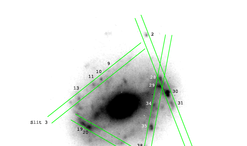
Figure 1: Location of the CGS4 slit positions used, together with identifications of the knots observed, marked on the $K$-band image of the nuclear region of M100 from Ryder & Knapen (1999). The 1.2 arcsec slit width is shown to scale.

Longslit spectroscopy of the central region of M100 was carried out over three nights from 1999 April 1-3 UT. Only limited data was acquired the first night due to heavy cirrus; conditions were photometric throughout the remaining two nights. The common-user near-IR spectrograph CGS4 (Mountain et al. 1990) on UKIRT with its 0.61 arcsec pixel scale, a 1.2 arcsec slit, and the 40 line mm^-1 grating in first order was employed, which delivers complete spectral coverage from 1.85–2.45 $\mu$m at a resolving power of 450. Using the images presented in Paper I, a total of 4 slit position angles and nuclear offsets were selected, covering at least 3 knots each; these are marked on Figure 1.

After taking the observations presented in Paper I, it became apparent that the infrared-emitting central region of M100 fills no more than one-third of the usable area of the detector array, and therefore, nodding to blank sky was not really necessary. For the observations presented here, sky subtraction was performed by sliding the objects of interest a total of 60 rows (36.6 arcsec) along the slit in between ‘object’ and ‘sky’ exposures. After setting the slit to the desired position angle, a manual search for the $K$-band nuclear peak was conducted, following which accurate offsets were applied by use of the UKIRT crosshead to place the slit right at the locations marked on Fig. 1. All observations of M100 were bracketed by similar sequences on the nearby A4 V star BS 4632, to enable removal of some of the telluric absorption features.

Data reduction was accomplished using a combination of tasks within the Starlink cgs4dr and NOAO iraf packages. After flatfielding, the difference of each object–sky pair was co-added into groups, with each grouped image representing $\sim 3000$ sec of on-source integration in the case of the M100 spectra, or $\sim 300$ sec for BS 4632. Any residual sky absorption/emission was removed from this image by fitting a low-order polynomial to galaxy-free regions within each row of the spatial axis. The high signal-to-noise of the stellar continuum in BS 4632 was used to define the width and curvature of suitable extraction apertures for both the ‘positive’ and ‘negative’ beams. After extracting matching apertures from an argon arc image, the spectra from both beams were wavelength calibrated separately to an accuracy of 0.2 nm. The spectrum of the negative beam was inverted, and then co-added in wavelength space to that of the positive beam. The strong Br$\gamma$ absorption intrinsic to BS 4632 was interpolated over, but this could not be done for Pa$\alpha$ or for Br$\delta$ due to their location near the trough of an H₂O absorption band.

Processing of the M100 knot spectra proceeded in a similar fashion, except that multiple apertures needed to be defined for each slit position. This was done in consultation with Fig. 1, but the exact aperture centres and widths were defined independently for each group. After extraction, wavelength calibration, and co-addition, the spectrum of each knot was divided by the BS 4632 spectrum which best matched the airmass of observation, and then multiplied by a blackbody curve corresponding to the temperature (8380 K) and flux density ($K=6.13$) of BS 4632. Table 1 summarises the observational parameters for each slit setting, including all of the knots that each slit was expected to intersect to some degree. The numbering sequence for the knots is as given in Table 1 of Paper I.

In order to define a consistent continuum right out into the region of extensive CO absorption beyond 2.3 $\mu$m, we fitted a power-law of the form $F_{\lambda}\propto\lambda^{\beta}$ to featureless sections of the spectrum near 2.11 and 2.27 $\mu$m (rest wavelength). After normalising each spectrum by this fit, the equivalent widths of the redshifted Pa$\alpha$, Br$\gamma$, and H₂ lines were measured using the SPLOT task in iraf, together with two determinations of the spectroscopic index CO_sp. The original definition of a CO spectroscopic index by Doyon, Joseph & Wright (1994a; hereafter DJW) has the form

$${\rm CO}_{\rm sp}^{\rm DJW}=-2.5\log\langle R_{2.36}\rangle$$ (1)

where $R_{2.36}$ is the mean normalised intensity between 2.31 and 2.40 $\mu$m in the rest frame of the galaxy (in the case of M100, this wavelength interval corresponds to $2.322-2.412$ $\mu$m). Although the output of both the DJW and the Leitherer et al. (1999; hereafter SB99) models use this definition of CO_sp, PDW advocated the adoption of a narrower wavelength interval over which to integrate, namely $2.2931-2.3200$ $\mu$m, which covers just the region from the band head to near the end of the 2–0 band. After a comprehensive analysis, this range was found to offer the best sensitivity to changes in luminosity class, and has also been endorsed by Hill et al. (1999). From equation 7 of PDW, we get the following relation between their definition of CO_sp and the equivalent width of CO (nm), measured over the rest wavelength interval $2.2931-2.3200$ $\mu$m:

$${\rm CO}_{\rm sp}^{\rm PDW}=-2.5\log\left(\frac{16.8-{\rm EW(CO,nm)}}{\eta}\right)$$ (2)

At the redshift of M100 (1571 ${\rm km~{}s}^{-1}$; Knapen et al. 1993), this wavelength interval becomes $2.305-2.332$ $\mu$m. Note that PDW give $\eta=16.6$, but our analysis in the Appendix shows that $\eta=16.9$ is more appropriate at our resolution.

3 Results

Figure 2 shows the spectra of the combined data for three of the knots, on which the main spectral features that have been measured are identified. Even at this resolution, the redshift of M100 is just enough to separate the Pa$\alpha$ emission line from the anomalous bump at 1.876 $\mu$m, which is a residual of the Pa$\alpha$ absorption in BS 4632. The (almost flat) continuum slope found in most of the knot spectra helps greatly in minimising the error that comes from fitting a power-law to the continuum and extrapolating it across the CO band.

Table 2 is a compilation of the measured equivalent widths and continuum power-law slopes $\beta$ for each of the knots which could be clearly distinguished in the spectra. Because of the tendency for CO${}_{\rm sp}^{\rm PDW}$ to underestimate CO${}_{\rm sp}^{\rm DJW}$ as noted in the Appendix, the former has been calculated using $\eta=16.9$ in equation 2. In order to gain a realistic estimate of the uncertainties, the equivalent width measurements were performed on each of the 3 or 4 individually-reduced groups (with exposure times of 2400–3800 sec), as well as the co-added result. The mean equivalent width adopted is that measured from the co-added spectra, while the error bars are based on the dispersion in the individual measurements. As expected, this shows that the uncertainties are dominated as much by the noise statistics and the subjective choice of extraction aperture as by the measurement errors and continuum fitting. Note that we have two independent observations and measurements of knot 28 (with slit 1 and, less optimally, slit 2), and except for the equivalent width of H₂, the results are consistent within the error bars.

It is also apparent that the error bars on measurements over the smaller PDW wavelength interval (their “extended” region) are significantly larger than the error bars on measurements over the full DJW range. These larger error bars, coupled with the need to then apply an empirical transformation, leads us to favour the use of CO${}_{\rm sp}^{\rm DJW}$ for comparison with the models. While the PDW definition undoubtedly is more robust than even narrower wavelength regions, and is more sensitive to changes in the stellar population, there appears to be little advantage to using it at our resolution. Our conclusions in the next section regarding the relative ages of the star-forming knots in M100 are unaffected by the choice of CO spectroscopic index.

Since the knots all have CO${}_{\rm sp}^{\rm DJW}$ in the range 0.20–0.28, we infer from Table 4 that the stellar populations of these knots are currently dominated by giants and/or supergiants of type K5 or later. We do not observe values of CO${}_{\rm sp}^{\rm DJW}$ quite as high as was measured for the ‘hotspots’ K1 and K2 in Paper I, which we attribute to the fact that the original spectroscopy did not target any particular knot, and that the continuum fitting was less rigorous.

4 Discussion

4.1 The Ages of the Starburst Knots

Figure 3 presents our results as a plot of CO spectroscopic index vs. the Br$\gamma$ equivalent width for the 16 knots (the two independent observations of knot 28 have been averaged), together with the loci of evolutionary synthesis models for starbursts as calculated by DJW, and used by PDW in age-dating the nuclear starburst in M83. There appears to be a well-defined sequence in the line strengths among the bulk of the knots, which parallels quite closely the starburst model with the shortest burst timescale $\tau$ (i.e. the “quasi-instantaneous” burst). Reading off the fiducial marks on this model indicates ages for these knots of between 8 and 10 Myr.

There is of course a selection effect here: the Br$\gamma$ equivalent width must be at least 0.2 nm to be detectable, so we can only put a lower age limit on knot 13. Similarly, there could be circumnuclear star-forming knots younger than 5 Myr around M100 which would be missed by our NIR imaging and spectroscopy, since there has not been sufficient time for the most massive stars to evolve to red supergiants. Nevertheless the observed upper envelope of Br$\gamma$ equivalent widths just below 1 nm suggests that there was an extended pause in star formation events $\sim 8$ Myr (on this model) ago. Furthermore, any bursts decaying at a rate slower than 5 Myr, and aged between 10 and 30 Myr ought also to be detectable, but none are seen.

We have also plotted our results on the closest equivalent SB99 models (Figure 4). The agreement between observations and the models is not as good as for the DJW models, but the two evolutionary tracks shown are the only two that come anywhere close to achieving the required values of CO${}_{\rm sp}^{\rm DJW}$. The first model is for an instantaneous burst of star formation (ISF), in which the IMF has a Salpeter-like form (slope $\alpha=2.35$ and upper mass cutoff of 100 M_⊙) and a metallicity of $2\times$ solar ($Z=0.04$). The alternative model is one which has a constant star formation rate (CSF) of 1 M_⊙ yr^-1, a steeper IMF ($\alpha=3.30$ and upper mass cutoff of 100 M_⊙) and a metallicity of twice-solar.

A high central metallicity in M100 is supported by H ii region spectroscopic abundance measurements by Skillman et al. (1996), who found $12+\log({\rm O}/{\rm H})\sim 9.3$ near the nucleus, or over $2.5\times$ solar metallicity. The tendency of existing models to predict CO spectroscopic indices which are too weak is a known problem (e.g., Devost & Origlia 1998; Origlia et al. 1999), and appears to be related to uncertainties in the effective temperatures and microturbulent velocities of the red supergiants, as well as the fraction of time these stars spend as blue supergiants during their core helium burning phase. Nevertheless, the evolutionary trend of the ISF model parallels quite closely the distribution of the knots, and even the age range of $6.5-7.0$ Myr is not inconsistent with that indicated by the DJW models, considering that the ISF model has $\tau<0.1$ Myr.

Although the (quasi-)instantaneous burst models fit the observed trend of knot line indices quite well, both Figures 3 and 4 leave open the possibility that a few of the knots could equally well just be due to steady (or only slowly declining) continuous star formation for the past 50–100 Myr. The same CSF model plotted in Fig. 4 predicts that in this age range, the knots should have colours $(J-H)=0.48\pm 0.02$ and $(H-K)=0.24\pm 0.02$, while the ISF model in the same figure predicts $(J-H)=0.46\pm 0.05$ and $(H-K)=0.22\pm 0.04$ for the age range 6.6–7.0 Myr. Each of these cases is fully consistent with the median of the dereddened knot colours, as plotted in Fig. 2 of Paper I, emphasising how ineffective broadband near-infrared colours are in distinguishing bursts from continuous star formation. As we show in Section 4.2.3, even knowledge of the H₂ 1–0 S(1) to Br$\gamma$ ratio still does not allow for an unambiguous distinction between instantaneous burst and continuous star formation models.

4.2 Other Hydrogen Lines

4.2.1 Pa$\alpha$

As Fig. 2 shows, the Pa$\alpha$ line at the redshift of M100 (1571 ${\rm km~{}s}^{-1}$) is clearly resolved from the rest-frame Pa$\alpha$ absorption in BS 4632. Thanks to the low water vapour column over Mauna Kea, measurements of Pa$\alpha$ are quite feasible despite the low atmospheric transmission at this wavelength, although the continuum level in this region is not as well fit by the power law. For this reason, the equivalent widths in Table 2 have been measured with respect to the base of the line profile, rather than the continuum as defined by an extrapolation of the power law with index $\beta$.

In Figure 5 we have plotted the equivalent width of the Pa$\alpha$ line against that of the Br$\gamma$ line. For Case B recombination of hydrogen at $T=10^{4}$ K (e.g. Table 4.2 of Osterbrock 1989), we would expect a ratio $I({\rm P}\alpha)/I({\rm Br}\gamma)=12.52$, as indicated by the dashed line (more metal-rich gas will be cooler, but even at $T=5\times 10^{3}$ K, the ratio is only slightly higher at 12.86). The fact that the Pa$\alpha$ line is consistently weaker than Br$\gamma$ would predict is usually attributed to reddening. However, the mean amount of extinction required to explain this difference (adopting the interstellar extinction curve from Cardelli, Clayton & Mathis 1989) is $A_{V}\sim 16$ mag, or $A_{K}\sim 1.8$ mag. This is a factor of 4 larger than the maximum extinction that was derived from the near-IR colour excesses of the knots in Paper I.

The equivalent width of an emission line ought to be independent of reddening, but this assumes that both the continuum flux and the line emission at a given wavelength originate from the same physical region; if the red supergiants had cleared much of the dust that shrouded their birth, then the stellar and nebular fluxes could experience quite different amounts of reddening. Alternatively, our corrections for Pa$\alpha$ absorption in the standard star, and for H₂O absorption in our atmosphere, may be inadequate. An added complication is the presence of extended, diffuse Pa$\alpha$ emission in the nuclei of many early-type galaxies (Böker et al. 1999; Alonso-Herrero et al. 2001). Clearly, despite being an order of magnitude stronger than Br$\gamma$, there are still a number of difficulties with using ground-based observations of the Pa$\alpha$ line as a star formation and reddening diagnostic.

4.2.2 H$\alpha$

The H$\alpha$ narrow-band imaging and Fabry-Pérot kinematics presented by Knapen et al. (1995a; 2000) reveal four main complexes of H ii regions forming an almost complete nuclear ring, coincident with that outlined by the $K$-band knots. Two of these complexes are associated with the major ‘hot-spots’ K1 and K2 at either end of the bar. On the basis of reduced dust obscuration, they suggested that K1 ought to be slightly older than K2, and indeed, our age analysis confirms that the aggregate of knots which make up K1 (knots 28-31) is slightly older than that of K2 (knots 19 and 20). Complexes H$\alpha 3$ and H$\alpha 4$, along the bar minor axis, are brighter than K1 and K2 in H$\alpha$, but dimmer in $K$, consistent with their being less evolved. As discussed in Section 4.1, the youngest knots are found near H$\alpha 3$ and H$\alpha 4$, providing further support for the qualitative age sequence of Knapen et al.

4.2.3 Molecular hydrogen

Molecular hydrogen emission in the H₂ 1–0 S(1) line at a rest wavelength of 2.122 $\mu$m is commonly observed in star-forming environments, but the nature of its excitation (shocks vs. UV fluorescence) is still somewhat ambiguous (e.g., Doyon, Wright & Joseph 1994b; Puxley, Ramsay Howat & Mountain 2000). When we plot the H₂ 1–0 S(1) line strengths against Br$\gamma$ (Figure 6), the two are clearly correlated (just as was demonstrated for the nuclei of a large sample of star-forming galaxies by Puxley, Hawarden & Mountain 1990), suggesting a close link between molecular hydrogen line emission and star formation in these knots. Table 2 lists the ratios of the H₂ 1–0 S(1) to Br$\gamma$ equivalent widths, and these are predominantly in the range $0.4-0.9$, very similar to the Puxley et al. (1990) ratios.

Using the same modeling framework as used for the evolutionary tracks in Fig. 3, Doyon et al. (1994b) showed that the S(1)/Br$\gamma$ ratio would not exceed 0.4 until at least 60 Myr after the onset of the burst, for $\tau=20$ Myr. The short ($\tau=1$ Myr) bursts favoured by Fig. 3 might be expected to achieve the observed S(1)/Br$\gamma$ ratios in Table 2 even earlier than 60 Myr. Their model assumes however that outflows from young stellar objects (YSOs) and from supernova remnants (SNRs) produce all of the H₂ line flux, whereas both UV fluorescence of photodissociation regions by massive stars, and large-scale shocks from the action of the spiral density wave, may also be significant sources in the centre of M100.

For comparison, their model with continuous star formation (like the CSF model of SB99 in Fig. 4) would barely exceed a ratio of 0.15, even after 100 Myr of evolution. Vanzi & Rieke (1997) measured ratios of this order in a sample of blue dwarf galaxies which, while representing perhaps the purest form of a starburst, may also be subject to the unknown effects of low metallicity. Thus, even a combined knowledge of the knot near-IR colours, their Br$\gamma$, H₂ and CO equivalent widths is still not sufficient to definitively exclude the possibility that at least some of the circumnuclear knots in M100 have been continuously forming stars for as long as 100 Myr.

4.3 Age trends

Table 3 lists the ages derived for each of the knots which lie on, or very near to the $\tau=1$ Myr locus of DJW in Fig 3. Four of the knots (2, 13, 28, and 38) lie well off this sequence, and it would appear that the bursts powering them are declining at a different rate from all the rest. Clearly, ages derived from the SB99 ISF model in Fig. 4 would be slightly younger, but the relative age sequence will still be the same. The location of each knot within the deprojected disk of M100 has been calculated using the disk orientation parameters ($i=27^{\circ}$, $\phi=153^{\circ}$) derived by Knapen et al. (1993) from their H i kinematic analysis. In Figure 7, we plot these ages against both radial distance and position angle in the plane of M100. In this sense, position angle increases counter-clockwise, with the origin lying midway between knots 20 and 37 in Fig 1.

We consider first the azimuthal age distribution. The knots at either end of the bar (19, 20 and 29) are all about the same age, $\sim 8.8$ Myr. The oldest knots (30, 31, 34, and 35) are located just south of the western end of the inner bar, while the youngest knots (9, 37 and 39) lie close to the bar minor axis, leading (or lagging) the oldest knots by $90^{\circ}$. Indeed, beginning at position angle $70^{\circ}$, there is the suggestion of an age sequence spanning at least a Myr as one circles the nuclear ‘ring’. A simple linear least squares fit (Press et al. 1992) to the age distribution, starting at position angle $70^{\circ}$, yields a Pearson’s $r$ value of $-0.75$ and Student’s $t$ probability of 0.005, the small value of which implies a significant correlation between position angle around the ring, and burst age. However, one could just as easily point to the appearance of two age minima (at position angles $50^{\circ}$ and $230^{\circ}$), but our limited sampling prevents us from identifying if there is a corresponding second age maximum near $300^{\circ}$. Nevertheless, Fig. 7 provides the first evidence that rather than being a stochastic process, circumnuclear star formation may be sequentially triggered.

At the radial distance of these knots, the orbital period given by the rotation curve of Knapen et al. (1993) is $\sim 20$ Myr, an order of magnitude larger than the observed age spread. Similarly, the bar pattern speed (determined independently by Knapen et al. (1995b) and by Wada et al. (1998)), $\Omega_{\rm p}\sim 65$ ${\rm km~{}s}^{-1}$ kpc^-1 leads to an even longer timescale. The maximum streaming velocities observed in H$\alpha$ and CO by Knapen et al. (2000) around the circumnuclear region are of order 40 ${\rm km~{}s}^{-1}$, too slow to causally connect the oldest and youngest star-forming knots. Thus, it cannot be the rotation of the bar, or bulk motion of the gas, which directly triggers the star formation.

The detailed nuclear morphology of M100, as pieced together from optical, near-infrared, H$\alpha$, and CO imaging, is analysed in great detail by Knapen et al. (1995a, b; 2000). They constructed a numerical model including gas, stars, and star formation, which successfully replicated many of the main features, including (1) the 1 arcmin stellar bar; (2) a pair of offset curved shocks, and streaming motions along the nuclear ‘ring’, both signatures of a global density wave induced by this bar; and (3) four distinct compression zones, two of which are close to the bar minor axis (where local maxima in the CO and H$\alpha$ emission are observed), and two near the ends of the bar where the spiral armlets are observed to switch from leading to trailing. As shown in fig. 15 of Knapen et al. (1995b), star formation at the ends of the bar in their model is seen to precede that along the minor axis (just as Fig. 7 suggests), but again the timescales involved are rather longer than the observed age spread.

One scenario worth considering would be an outward propagating shock-wave, which reaches the ends of the bar first, then sets off the knots along the bar minor axis a short while later, resulting in a radial age gradient. As Fig. 7 shows, the oldest knots do tend to be at larger radii, but then so too is the youngest, so the evidence is less compelling (for a linear least squares fit, $r=0.22$ and $t=0.5$). What makes this model attractive though, is that a shock wave velocity of only $\sim 200$ ${\rm km~{}s}^{-1}$ is required to explain the observed age spread, compared with up to 1000 ${\rm km~{}s}^{-1}$ for a density wave-driven shock propagating around the ring. In addition, a one-off outburst such as this makes it easier to account for the apparent recent pause in star formation events, whereas a persistent phenomenon (such as a spiral density wave for instance) would be expected to have produced a much larger spread in burst ages than is observed in M100.

5 Conclusions

New longslit $K$-band spectroscopy of the circumnuclear region of M100 has been obtained, targeting specifically the compact ‘knots’ identified from high-resolution near-IR imaging in Paper I. We have shown that even at comparatively low resolution ($R\sim 450$), it is possible to discern age differences of as little as 0.2 Myr in circumnuclear star forming regions by comparing the equivalent widths of the Br$\gamma$ emission line with the CO 2.29 $\mu$m absorption band. While the primary age sequence diagnostic is the CO spectroscopic index, complementary measurements of the Br$\gamma$ and H₂ 1–0 S(1) lines allows us to distinguish short-duration, rapidly declining bursts from continuous star formation. Comparison with starburst models from the literature indicates that the bulk of the circumnuclear star formation events in M100 are best accounted for by the former, with decay timescales of $\sim 1$ Myr.

We find the strongest evidence yet that circumnuclear star formation in M100 is sequentially triggered in an azimuthal or radial sense (or perhaps both). While the absolute ages of the knots are highly model-dependent, the age spread is unambiguous. The youngest and oldest knots are quite spatially distinct, but the physical separations and timescales involved are such that only shocks with velocities of a few hundreds of kilometres per second can causally connect them. The presence of curved dust lanes bisecting the circumnuclear ring verifies the existence of large-scale shocks in this region, most likely driven by a bar-induced spiral density wave. However, the symmetry of the age distribution is such that a simple, radially-propagating shock may just as easily explain the situation, though no source can yet be identified.

To date, we have secured spectra for 16 of the 43 knots identified in Paper I, and of these, only 12 are suitable for constraining the age distribution. To confirm our suspicion of an azimuthal age gradient (or even a cycle) in M100 will require better sampling of some of the fainter knots in M100 (something for which the new generation of near-infrared multi-object spectrographs and integral-field units will be ideally suited). Few galaxies have had their circumnuclear kinematics and star formation studied in as much detail as M100 has, but more are clearly needed if we are to understand the role of the bar in influencing both.

Figure 2: Reduced spectra for three of the knots in M100, illustrating the relative changes in line strengths going from a relatively young knot (Knot 9, age $\sim 8.4$ Myr) to one of the oldest knots (Knot 30, age $\sim 9.6$ Myr), via one of intermediate age (Knot 20, age $\sim 8.8$ Myr). The main spectral features are marked, as well as the two wavelength regions over which the CO equivalent width was measured: (upper line) the range defined by DJW, and (lower line) the narrower range adopted by PDW. The bump on the blue wing of the Pa$\alpha$ lines is a residual of the Pa$\alpha$ 1.876 $\mu$m absorption intrinsic to the telluric standard star. The residual due to Br$\delta$ at 1.945 $\mu$m has been patched over in these spectra.

Figure 3: Observed CO spectroscopic indices plotted against the Br$\gamma$ equivalent widths for 16 of the star-forming knots in M100. The two independent observations of knot 28 in Table 2 have been combined with a weighted average, to give the point at $(-0.73,0.23)$. Also shown in this plot are the evolutionary tracks for three starburst models as presented in Fig. 3 of PDW, with exponentially-decreasing star formation timescales $\tau=1$, 5, and $20\times 10^{6}$ yr. The points marked on the tracks indicate the time taken in Myr to reach that point from the onset of the burst.

Figure 4: As for Figure 3, but this time using two evolutionary tracks from Leitherer et al. (1999) models. The track marked “ISF” is for a $Z=0.04$, $\alpha=2.35$, M${}_{\rm up}=100$ M_⊙ instantaneous burst model, while the one marked “CSF” is for a $Z=0.04$, $\alpha=3.30$, M${}_{\rm up}=100$ M_⊙ model with continuous star formation at a rate of 1 M_⊙ yr^-1. The points marked on the tracks indicate the time taken in Myr to reach that point from the onset of star formation.

Figure 5: The equivalent width of the Pa$\alpha$ emission line from each of the knots plotted against the Br$\gamma$ equivalent width. The relationship expected from Case B recombination line theory is shown by the dashed line. The two independent observations of knot 28 in Table 2 have been combined with a weighted average, to give the point at $(-0.73,0.29)$.

Figure 6: The equivalent width of the H₂ 1–0 S(1) emission line from each of the knots plotted against the Br$\gamma$ equivalent width. The two independent observations of knot 28 in Table 2 have been combined with a weighted average, to give the point at $(-0.73,-0.48)$.

Figure 7: The derived ages for the 12 knots in M100 which appear to best follow the evolutionary trend of the $\tau=1$ Myr burst locus in Fig. 3, plotted against deprojected radius (top) and azimuth (bottom) in the disk of M100. The zero-point of the position angle scale corresponds to the kinematical major axis $\phi=153^{\circ}$ (roughly halfway between knots 20 and 37 in Fig. 1), and position angle increases going counter-clockwise.

Appendix A The CO Index in Stars

Since many of the studies to date of the strength of CO absorption in starburst systems have been with resolving powers at least twice that which we have used here, we felt it was important to verify that we would not lose any sensitivity to stellar effective temperature or luminosity class. To this end, we set out to observe a variety of late-type stars covering nearly the full range of spectral type later than F5, with the same observational setup as for the observations of M100. Observing time constraints, coupled with the difficulty in finding cool stars with well-defined spectral types which were not so bright as to saturate the detector, precluded us from going below $T_{\rm eff}=3400$ K. Table 4 gives the observed CO_sp values for both definitions (equations 1 and 2), as well as the spectral classification from Hoffleit (1982), the derived stellar effective temperature from Schmidt-Kaler (1982), and the continuum power-law slope $\beta$. Figure 8 presents the results for our stellar dataset, along with the relations for dwarfs, giants, and supergiants empirically-determined by DJW from the stellar atlas of Kleinmann & Hall (1986).

Although our measurements match the expected trends quite well for the hotter stars, there is considerably more scatter than for the equivalent plot in DJW (their Fig. 7). In order to assess how much of this scatter is due to our resolution, and how much may be intrinsic to the stars themselves, we have made use of the $K$-band stellar spectral library of Wallace & Hinkle (1997). We measured CO${}_{\rm sp}^{\rm DJW}$ in all of their luminosity class I, III, and V stars with $3000<T_{\rm eff}<6000$ K that were not also in the Kleinmann & Hall (1986) study. As Figure 9 shows, even at higher resolution ($R\sim 3000$) there is indeed somewhat more scatter in CO spectroscopic index with type and luminosity class than one might conclude from the analysis of DJW, particularly amongst the bright supergiants (a similarly enhanced degree of scatter amongst the supergiants is exhibited by the independent sample of Förster Schreiber 2000). While this does provide some reassurance that lower resolution does not significantly compromise our ability to measure real changes in CO${}_{\rm sp}^{\rm DJW}$ with changing stellar population, the large scatter (up to 0.1 dex) about the mean relation defined for supergiants by DJW ought to be of concern. The supergiants, when present, will dominate CO${}_{\rm sp}^{\rm DJW}$, and the predictions of the models assume a much tighter relation between CO${}_{\rm sp}^{\rm DJW}$ and $T_{\rm eff}$ like the one found by DJW.

One aspect that may be resolution-dependent is the conversion from CO equivalent width over the narrow wavelength interval used by PDW, and the equivalent CO spectroscopic index (equation 2). Lowering the resolution will tend to broaden the CO bandhead, and the wavelength limits may no longer encompass the same extent of the line profile. The much larger wavelength interval used by DJW will be less susceptible to this effect. Indeed, when we plot CO_sp using both definitions for our own observations of field stars, as well as all the M100 knots (Figure 10), it is apparent that CO${}_{\rm sp}^{\rm DJW}$ is consistently less than CO${}_{\rm sp}^{\rm PDW}$ by $\sim 0.02$ dex when equation 2 is used with $\eta=16.6$. Hill et al. (1999) found a similar tendency to underestimate CO${}_{\rm sp}^{\rm PDW}$ in their $R\sim 400$ spectra. We can compensate for this by using $\eta=16.9$ in equation 2 to restore good agreement between the two indices.

Table 4: Stellar Parameters and CO Spectroscopic Indices

Star	Type	$\beta$	$T_{\rm eff}$	CO${}_{\rm sp}^{\rm DJW}$	CO${}_{\rm sp}^{\rm PDW}$
BS 7503	G1.5 Vb	-1.5	5900	0.00	-0.01
BS 6697	G2 V	-1.4	5860	0.01	-0.01
BS 6538	G5 V	-1.4	5770	0.01	-0.01
BS 6301	K0 V	-1.3	5250	0.04	0.02
BS 6806	K2 V	-1.6	4900	0.03	0.00
BS 8085	K5 V	-1.2	4350	0.06	0.05
BS 8086	K7 V	-1.1	4060	0.06	0.06
BS 6531	F6 III	-1.7	6360	0.00	-0.02
BS 6466	G0 III	-1.6	5850	0.04	0.02
BS 6239	G5 III	-1.5	5150	0.04	0.01
BS 6287	G8 III	-1.9	4900	0.04	0.02
BS 6307	K0 III	-1.4	4750	0.07	0.04
BS 6358	K5 III	-2.0	3950	0.14	0.12
BS 6159	K7 III	-2.3	3850	0.17	0.15
BS 7244	M0 III	-2.4	3800	0.18	0.12
BS 6834	M4 IIIab	-2.1	3430	0.24	0.20
BS 8752	G4 0	-0.5	4970	0.00	0.00
BS 6713	K0.5 IIb	-2.2	4530	0.10	0.08
BS 6498	K2 II	-2.1	4340	0.16	0.14
BS 2615	K3 Ib	-1.8	4080	0.16	0.13
BS 6693	M1 Ib	-1.6	3550	0.26	0.21

Figure 8: Observed variation of the CO spectroscopic index CO${}_{\rm sp}^{\rm DJW}$ (measured over the original wavelength range proposed by DJW) with spectral type and luminosity class in nearby field stars. Compare this figure with the equivalent plot in Appendix A of DJW, which employed the spectral atlas of Kleinmann & Hall (1986). The plotted curves are the relations between CO${}_{\rm sp}^{\rm DJW}$ and $T_{\rm eff}$ determined by DJW for each luminosity class.

Figure 9: As for Figure 8, but using the $R\sim 3000$ stellar spectral atlas of Wallace & Hinkle (1997).

Figure 10: Comparison of the CO spectroscopic indices in nearby field stars and in the M100 knot spectra. CO${}_{\rm sp}^{\rm DJW}$ are the direct integrated measurements between rest wavelengths of 2.31–2.40 $\mu$m, while CO${}_{\rm sp}^{\rm PDW}$ are measurements over the rest wavelength range 2.293–2.320 $\mu$m which are then converted to the equivalent full-range value. The dashed line indicates what would be a 1:1 correspondence.

References

- [1] Alonso-Herrero A., Ryder S. D., Knapen J. H., 2001, MNRAS, in press (astro-ph/0010522)
- [2] Böker T., Calzetti D., Sparks W., Axon D., Bergeron L.E., Bushouse H., Colina L., Daou D., Gilmore D., Holfeltz S., MacKenty J., Mazzuca L., Monroe B., Najita J., Noll K., Nota A., Ritchie C., Schultz A., Sosey M., Storrs A., Suchkov A., 1999, ApJS, 124, 95
- [3] Cardelli J. A., Clayton G. C., Mathis J. S., 1989, ApJ, 345, 245
- [4] Devost D., Origlia L., 1998, in Friedli D., Edmunds M., Robert C., Drissen L., eds., ASP Conf. Ser. Vol. 147, Abundance Profiles: Diagnostic Tools for Galaxy History. Astron. Soc. Pac., San Francisco, p. 201
- [5] Doyon R., Joseph R. D., Wright G. S., 1994a, ApJ, 421, 101 (DJW)
- [6] Doyon R., Wright G. S., Joseph R. D., 1994b, ApJ, 421, 115
- [7] Förster Schreiber N. M., 2000, astro-ph/0007324
- [8] Hill T. L., Heisler C. A., Sutherland R., Hunstead R. W., 1999, AJ, 117, 111
- [9] Hoffleit D., 1982, Bright Star Catalogue (4th edtn.). Yale Univ. Observatory, New Haven, CT
- [10] Kleinmann S. G., Hall D. N. B., 1986, ApJS, 62, 501
- [11] Knapen J. H., Beckman J. E., Shlosman I., Peletier R. F., Heller C. H., de Jong R. S., 1995a, ApJ, 443, L73
- [12] Knapen J. H., Beckman J. E., Heller C. H., Shlosman I., de Jong R. S., 1995b, ApJ, 454, 623
- [13] Knapen J. H., Cepa J, Beckman J. E., Soledad del Rio M., Pedlar A., 1993, ApJ, 416, 563
- [14] Knapen J. H., Shlosman I., Heller C. H., Rand R. J., Beckman J. E., Rozas M., 2000, ApJ, 528, 219
- [15] Kotilainen J. K., Reunanen J., Laine S., Ryder S. D., 2000, A&A, 353, 834
- [16] Leitherer C., Schaerer D., Goldader J. D., González Delgado R. M., Robert C., Foo Kune D., de Mello D. F., Devost D., Heckman T., 1999, ApJS, 123, 3 (SB99)
- [17] Mountain C. M., Robertson D. J., Lee T. J., Wade R., 1990, Proc. SPIE, 1235, 25
- [18] Origlia L., Goldader J. D., Leitherer C., Schaerer D., Oliva E., 1999, ApJ, 514, 96
- [19] Origlia L., Oliva E., 2000, A&A, 357, 61
- [20] Osterbrock D. E., 1989, Astrophysics of Gaseous Nebulae and Active Galactic Nuclei. University Science Books, Mill Valley, CA
- [21] Press W. H., Teukolsky S. A., Vetterling W. T., Flannery B. P., 1992, Numerical Recipes (Second Edition), Cambridge University Press, Cambridge
- [22] Puxley P. J., Doyon R., Ward M. J., 1997, ApJ, 476, 120 (PDW)
- [23] Puxley P. J., Hawarden T. G., Mountain C. M., 1990, ApJ, 364, 77
- [24] Puxley P. J., Ramsay Howat S. K., Mountain C. M., 2000, ApJ, 529, 224
- [25] Reunanen J., Kotilainen J. K., Laine S., Ryder S. D., 2000, ApJ, 529, 853
- [26] Ryder S. D., Knapen J. H., 1999, MNRAS, 302, L7 (Paper I)
- [27] Schmidt-Kaler T., 1982, in Schiaffers K., Voight H. H., eds, Landolt-Börnstein Numerical Data and Functional Relationships in Science & Technology, Vol. 2: Astronomy and Astrophysics, Subvolume b, Stars & Star Clusters. Springer, NY
- [28] Skillman E. D., Kennicutt R. C., Shields G. A., Zaritsky D., 1996, ApJ, 462, 147
- [29] Vanzi L., Rieke G. H., 1997, ApJ, 479, 694
- [30] Wada K., Sakamoto K., Minezaki T., 1998, ApJ, 494, 236
- [31] Wallace L., Hinkle K., 1997, ApJS, 111, 445