Populating a cluster of galaxies – I. Results at $z=0$

Abstract

We simulate the assembly of a massive rich cluster and the formation of its constituent galaxies in a flat, low-density universe. Our most accurate model follows the collapse, the star-formation history and the orbital motion of all galaxies more luminous than the Fornax dwarf spheroidal, while dark halo structure is tracked consistently throughout the cluster for all galaxies more luminous than the SMC. Within its virial radius this model contains about $2\times 10^{7}$ dark matter particles and almost 5000 distinct dynamically resolved galaxies. Simulations of this same cluster at a variety of resolutions allow us to check explicitly for numerical convergence both of the dark matter structures produced by our new parallel N-body and substructure identification codes, and of the galaxy populations produced by the phenomenological models we use to follow cooling, star formation, feedback and stellar aging. This baryonic modelling is tuned so that our simulations reproduce the observed properties of isolated spirals outside clusters. Without further parameter adjustment our simulations then produce a luminosity function, a mass-to-light ratio, luminosity, number and velocity dispersion profiles, and a morphology-radius relation which are similar to those observed in real clusters. In particular, since our simulations follow galaxy merging explicitly, we can demonstrate that it accounts quantitatively for the observed cluster population of bulges and elliptical galaxies.

1 Introduction

The last two decades have witnessed substantial progress towards an understanding of hierarchical galaxy formation within the framework of a universe dominated by cold dark matter (CDM). For an appropriate choice of the cosmological parameters, the CDM theory provides a remarkably successful description of large-scale structure formation, and it is in good agreement with a large variety of observational data. Much of this progress has been achieved by detailed analytical and numerical studies of the collisionless dynamics of the dark matter. As a result, this part of cosmic evolution is now quite well understood. However, the actual formation of the luminous parts of galaxies within CDM universes involves many complex physical processes in addition to gravity, for example, shocking and cooling of gas, and star formation with its attendant regulation and feedback mechanisms. The theoretical modeling of important aspects of these processes is still highly uncertain.

Not surprisingly, the lack of precise specifications for treating the relevant physics has also hampered direct numerical studies of galaxy formation. In addition, such studies are confronted with the huge range of scales over which these physical processes interact. Difficulties in finding robust and appropriate algorithms for handling “subgrid” physics have so far prevented hydrodynamical simulations from reproducing many basic properties of galaxies, although more recent work is beginning to achieve some notable successes both for individual galaxies (e.g. Katz & Gunn 1991; Navarro & White 1994; Steinmetz & Müller 1995; Mihos & Hernquist 1996; Walker et al. 1996; Navarro & Steinmetz 1997; Steinmetz & Navarro 1999) and for the distribution of galaxy populations (e.g. Cen & Ostriker 1993, 2000; Katz et al. 1996, 1999; Weinberg et al. 1997, 2000; Steinmetz & Müller 1995; Blanton et al. 1999; Pearce et al. 1999, 2000).

Much of our current understanding of galaxy formation has been learned through ‘semi-analytic’ techniques, as laid out originally by White & Frenk (1991), Cole (1991) and Lacey & Silk (1991), building on the scenario first sketched by White & Rees (1978). In these models, each of the complicated and interacting physical processes involved in galaxy formation is approximated using a simplified, physically based model. These processes include the growth through accretion and merging of dark matter haloes, the shock heating and virialization of gas within these haloes, the radiative cooling of gas and its settling to a rotationally supported disk, star formation, and the resulting feedback from supernovae and stellar winds, the evolution of stellar populations, absorption and reradiation by dust, and galaxy merging with its accompanying starbursts and morphological transformations. At the expense of uncertainties introduced by the simplifying assumptions, semi-analytic techniques can access a much larger dynamic range than numerical simulations, they allow a fast exploration of parameter space and of the influence of the specific simplifying assumptions chosen, and they facilitate direct comparisons with a wide range of observational data.

Over the last few years, a number of groups have used semi-analytical models to study galaxy formation, and to interpret observations of galaxy populations at low and high redshift (Lacey et al. 1993; Kauffmann et al. 1993, 1994; Cole et al. 1994; Heyl et al. 1995; Baugh et al. 1996a, b; Kauffmann 1995a, b, 1996a, 1996b; Guiderdoni et al. 1998; Kauffmann & Charlot 1998; Baugh et al. 1998, 1999; Mo et al. 1998, 1999; Devriendt et al. 1998; Somerville & Primack 1999; Kauffmann & Haehnelt 2000; Cole et al. 2000; van den Bosch 2000; Boisser & Prantzos 2000; Haehnelt & Kauffmann 2000; Somerville et al. 2000). Stellar population synthesis modelling allows detailed photometric comparison with observation, including studies of the strong evolution apparent in observed high redshift galaxy samples. With a small number of free parameters, semi-analytic models have been quite successful in allowing a unified and coherent interpretation of a broad range of galaxy properties, for example, luminosity functions, Tully-Fisher and Faber-Jackson relations, number counts, the distributions of morphology, color and size, global and individual star formation histories, background radiation contributions from the UV to the far IR, clustering strengths, and the observed relations between AGN’s and their host galaxies. Most studies concentrate on a few specific issues. Oversimplifications in the adopted physical models often show up as inconsistencies with observation in other areas. For example, until recently most studies had difficulty simultaneously to fit the zero-point of the Tully-Fisher relation and the luminosity function of field galaxies. Recent work has removed some of the most serious oversimplifications in this area and has reduced the discrepancy significantly (Somerville & Primack 1999; van den Bosch 2000).

The construction of dark matter merging history trees (Kauffmann & White 1993; Somerville & Kolatt 1999; Sheth & Lemson 1999) is an important ingredient in semi-analytic models. In most studies, Monte-Carlo realizations of merging histories for individual objects are generated using the extended Press-Schechter formalism (Press & Schechter 1974; Bond et al. 1991; Lacey & Cole 1993). A disadvantage of this approach is that there is little information about the spatial distribution of galaxies, although two point correlations can be estimated using the methods introduced by Mo & White (1996) (see also Baugh et al. 1999). In order to study clustering in more detail semi-analytic models have been combined with cosmological N-body simulations; the galaxy population within each of the virialised haloes present in a given output of the simulation is created by a Monte Carlo “semi-analytic” realisation of its prior history and these galaxies are then attached to the halo centre and to random “satellite” particles within the halo (Kauffmann et al. 1997; Governato et al. 1998; Benson et al. 2000a, b; Wechsler et al. 2000). This allows mock catalogues of galaxies to be constructed which contain all the spatial and kinematic information of real redshift surveys.

In a natural extension of this approach, one can use N-body simulations not only to provide the mass distribution at a given time, but also to reconstruct individual halo merging histories, a scheme first tried in a crude form by White et al. (1987). This allows one to avoid the uncertainties inherent in the Press-Schechter formalism, and it provides spatial and kinematic distributions not just for the final galaxies but for their progenitors at all earlier times as well. Thus it is effectively equivalent to a full dynamical simulation of galaxy formation and clustering, but with the advantage that the computationally intensive part of the procedure, the original N-body simulation, does not need to be repeated every time the assumptions about baryonic processes are changed. The disadvantages in comparison with the simpler scheme just discussed are that the resolution of the merging history trees is limited by that of the N-body simulation and that particle data must be stored sufficiently often for the trees to follow adequately the growth of structure. The method thus requires frequent data dumps from high resolution simulations of cosmologically representative volumes, leading to a substantial raw data volume.

Recently, Roukema et al. (1997) studied merging history trees directly from N-body simulations using scale-free simulations and a rather limited number of simulation outputs. A much more extensive study has been published by Kauffmann et al. (1999a, hereafter KCDW), who constructed merging history trees from two high-resolution N-body simulations using a total of 51 output times between redshift $z=20$ and $z=0$. KCDW grafted semi-analytic models of galaxy formation onto the simulated merger trees to study how the clustering of galaxies is related to intrinsic properties like luminosity, colour and morphology. In subsequent papers, they used this methodology to predict the evolution of clustering to high redshift (Kauffmann et al. 1999b), to construct realistically selected mock redshift surveys (Diaferio et al. 1999), and to study the spatial and kinematic distributions of galaxies within clusters (Diaferio et al. 2000).

Using a somewhat different technique, van Kampen et al. (1999) also made use of the full merging history of N-body simulations. They modified an existing N-body code so that heavier ‘tracer’ particles were introduced during the execution of the simulation. These tracer particles, identified with galaxies, replaced locally overdense groups of the orginal particles. This approach neglects the internal structure of galaxy/halo systems, for example the fact that such systems can be stripped of much of their mass as they orbit within a cluster. In addition it is somewhat inflexible since any change in the assumptions about how baryonic part of galaxies forms and evolves requires the simulation to be repeated.

Our approach follows the methodology of KCDW, extending it to deal with higher resolution simulations. In such simulations, substantial substructure, partially stripped haloes of cluster galaxies, can be identified within dark matter clumps corresponding to galaxy groups and clusters. To this end, we study four simulations of the formation of a rich cluster of galaxies. These simulations follow the same object, a Coma-like cluster of mass $8\times 10^{14}\,\,h^{-1}{\rm M}_{\odot}$ in a flat, low-density universe, but use different mass resolutions. We resolve the virial region of the final cluster with $0.12$, $0.61$, $3.5$ and $20$ million particles, respectively, and we sample the field in the region immediately around the cluster at the same resolution but with about twice as many particles in each case. The cosmological tidal field is represented by an additional boundary region with $\sim 3.1$ million particles extending to a distance of $70\,h^{-1}{\rm Mpc}$ from the cluster. This sequence allows us to test explicitly how our results depend on numerical resolution.

We develop a new algorithm, SUBFIND, for identifying substructure within the clumps formed in these simulations. This algorithm defines ‘subhaloes’ as locally overdense, self-bound particle groups, and is able to detect hierarchies of substructure using just a single simulation output. As in KCDW, we have stored 51 simulation snapshots from $z=20$ to the current epoch, and we trace the merging history of groups and their subhaloes from output to output. We modify the semi-analytic recipes employed by KCDW to allow the inclusion of subhaloes, and we analyse the changes resulting from this increase in fidelity to the physical system modelled.

In particular, we study the luminosity function of the cluster, its mass-to-light ratio, the Tully-Fisher relation of spirals in the surrounding field, the Faber-Jackson relation of field and cluster ellipticals, and the $B-V$ colors of our model galaxies. We show that the new subhalo-scheme gives rise to a pronounced radial segregation by morphology. We investigate luminosity segregation by comparing the radial profiles of galaxies by number, morphology and luminosity with that of the dark matter. Finally, we study how the velocity dispersion profile of the galaxies depends on their luminosity and colour and compare it with the corresponding quantity for the dark matter. For all these quantities we are able to demonstrate good numerical convergence for all galaxies brighter than the SMC.

Our approach also allows a detailed study of the formation history of the cluster and its galaxies. In particular, we have analysed the star formation history of field and cluster galaxies, the spatial and temporal origin of the ‘first’ stars that end up in the cluster (White & Springel 1999), and the evolution of the merger rate of galaxies. These results are discussed in a companion paper.

Interestingly, the new subhalo analysis improves the agreement with observational data, especially with respect to the cluster luminosity function. Most of the bright galaxies in the final, highly-resolved cluster are still connected to well localized subhaloes within the smooth dark matter background of the cluster. There is hence no need to estimate merging timescales within the cluster using dynamical friction or approximate cross-section arguments. Mergers are treated automatically in a fully dynamically consistent way. As we will discuss, inaccuracies in estimated merging times can lead to a problem of excessively bright first ranked cluster galaxies in the simpler methodology which does not track subhaloes. This problem goes away in our refined approach which also demonstrates explicitly that merging can account for the observed fractions of elliptical and bulge-dominated galaxies and for their distribution within clusters.

This paper is organized as follows. In Section 2 we describe the N-body simulations, and in Section 3 we review the techniques of KCDW, and our specific implementation of them. In Section 4 we discuss our techniques for identifying dark matter substructure within larger haloes, and our methods of tracing it from output to ouput in the simulations. We then describe the implementation of semi-analytic models including this subhalo information, and we present results obtained with these prescriptions in Section 5. Finally, we discuss some aspects of our findings in Section 6.

2 Cluster simulations

In this study, we analyse collisionless simulations of clusters of galaxies that are generated by the technique of ‘zooming in’ on a region of interest (Tormen et al. 1997). In a first step, a cosmological simulation with sufficiently large volume is used to allow the selection of a suitable target cluster. For this purpose, we employed the GIF-$\Lambda$CDM model carried out by the Virgo consortium. It has cosmological parameters $\Omega_{0}=0.3$, $\Omega_{\Lambda}=0.7$, $h=0.7$, spectral shape $\Gamma=0.21$, and was cluster-normalized to $\sigma_{8}=0.9$. The simulation followed $256^{3}$ particles of mass $1.4\times 10^{10}h^{-1}{\rm M}_{\odot}$ within a comoving box of size $141.3\,h^{-1}{\rm Mpc}$ on a side. Note that this simulation is one of the models recently studied by KCDW. We selected the second most massive cluster that had formed in the GIF simulation for further study. This cluster has a virial mass $8.4\times 10^{14}\,h^{-1}{\rm M}_{\odot}$, and it appears to be well relaxed at the present time.

Table 1: Numerical parameters of our cluster simulations. All four simulations compute the evolution of the same cluster, assuming a $\Lambda$CDM universe with cosmological parameters $\Omega_{0}=0.3$, $\Omega_{\Lambda}=0.7$, $\Gamma=0.21$, $\sigma_{8}=0.9$, and $h=0.7$. The simulations follow a sphere of matter with comoving diameter $141\,h^{-1}{\rm Mpc}$. In the Table, we give the particle mass $m_{\rm p}$ used in the central high-resolution zone, the starting redshift $z_{\rm start}$, the gravitational softening $\epsilon$ in the high-resolution zone, the number $N_{\rm hr}$ of high-resolution particles, the number $N_{\rm bnd}$ of boundary particles, the total number $N_{\rm tot}$ of particles, and the number $N_{\rm p}$ of processors used in each of the simulations S1-S4. The gravitational softening was kept fixed at the given values in physical coordinates below redshift $z=9$, and in comoving coordinates above this redshift.

	S1	S2	S3	S4
$m_{\rm p}\;[\,h^{-1}{\rm M}_{\odot}]$	$6.87\times 10^{9}$	$1.36\times 10^{9}$	$2.38\times 10^{8}$	$4.68\times 10^{7}$
$z_{\rm start}$	30	50	80	140
$\epsilon\;[\,h^{-1}{\rm kpc}]$	6.0	3.0	1.4	0.7
$N_{\rm hr}$	450088	1999978	12999878	66000725
$N_{\rm bnd}$	3029956	3117202	3016932	3013281
$N_{\rm tot}$	3480044	5117180	16016810	69014006
$N_{\rm p}$	16	32	128	512

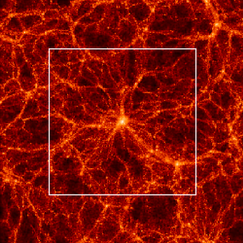
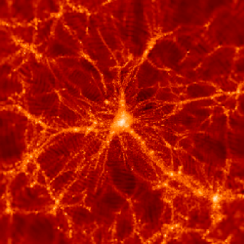
Figure 1: The projected mass density fields in slices of thickness 10$\,h^{-1}{\rm Mpc}$ around the cluster center in the original GIF simulation (left), and in the S3 resimulation (right). The left image is $141\,h^{-1}{\rm Mpc}$ on a side, and the white square marks the region ($85\,h^{-1}{\rm Mpc}$ on a side) that is displayed in the image of the resimulation on the right. In the right panel, you may notice small traces of the spherical grid used to represent the density field in the boundary region. Note that these residuals of the grid structure are just seen because of projection effects that arise in the visualization technique.

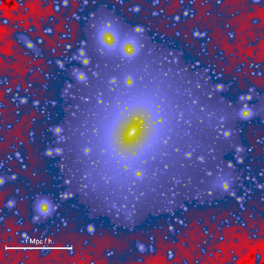
Figure 2: The dark matter distribution of the S4 cluster at $z=0$. The image shows all the mass in a box of sidelength $4\,h^{-1}{\rm Mpc}$ around the cluster center. To render the substructure visible, particles have been weighted by their local density (computed by adaptive kernel estimation), and a logarithmic color scale has been applied. Note that the small bright dots that are visible in the cluster should not be mistaken as noise – they are in fact self-bound subhaloes and correspond to surviving cores of haloes that have fallen into the cluster at some earlier time.

In a second step, we simulated the formation of this cluster again, using greatly increased mass and force resolution. To this end, the particles in the final GIF-cluster and in its immediate surroundings were traced back to their Lagrangian region in the initial conditions. The corresponding part of the displacement field was then sampled using a glass-like particle distribution with smaller particle masses than in the GIF simulation. Due to the increase in resolution, the fluctuation spectrum could now be extended to smaller scales. We added a random realization of this additional small-scale power, while we kept all the waves on larger scales that had been used in the GIF simulation.

Outside this central high-resolution region, we gradually degraded the resolution by using particles with masses that grow with distance from the center. In this ‘boundary region’, we employed a spherical grid whose spacing grew with distance from the high resolution zone. The spherical boundary region extends to a total diameter of $141.3\,h^{-1}{\rm Mpc}$, which is just the box size of the original GIF simulation. Beyond this region, we assumed vacuum boundary conditions, i.e. a vanishing density fluctuation field. Using comoving coordinates, we then evolved the simulations to redshift $z=0$ with our new parallel tree-code GADGET. This code uses individual timesteps for all particles, and was designed to run on massively parallel supercomputers with distributed memory. Parallelization is achieved explicitly using the communication library of the Message Passing Interface (MPI). A full account of the numerical and algorithmic details of GADGET is given elsewhere (Springel et al. 2000).

To be able to study systematic effects arising from numerical resolution, we simulated the same cluster several times, increasing the resolution step by step. In the first step, refered to as simulation ‘S1’ from here on, the particle mass was just about two times smaller than in the original GIF simulation. For the high-resolution zone of S1, we used a total of 450000 particles and a gravitational softening of $\epsilon=6.0\,h^{-1}{\rm kpc}$. The boundary region was represented with an additional $\sim 3$ million particles. This relatively high number of boundary particles was chosen with the sequence of our planned simulations in mind. Except for slight changes at its inner rim, we kept the sampling of the boundary region fixed for the other simulations, where we populated the central zone with many more particles. In simulation ‘S2’, we used 2 million high-resolution particles, and we reduced the gravitational softening to $3.0\,h^{-1}{\rm kpc}$. In simulation ‘S3’, we employed a total of 13 million high-resolution particles with mass $2.4\times 10^{8}\,h^{-1}{\rm M}_{\odot}$, and a softening of $1.4\,h^{-1}{\rm kpc}$. Finally, in simulation ‘S4’ we used 66 million particles for the high-resolution zone, pushing the particle mass down to $4.68\times 10^{7}\,h^{-1}{\rm M}_{\odot}$ and the spatial resolution down to $0.7\,h^{-1}{\rm kpc}$. In each case, roughly one third of the particles in the high-resolution zone ends up in the virialized region of the final cluster. This means that S4 resolves a single object with about 20 million particles.

In Table 1, we summarize important numerical parameters of our simulations. Note that we have softened gravity using a spline kernel. Our cited values for $\epsilon$ are such that the gravitational potential of a point mass at zero lag is $\Phi=-Gm/\epsilon$, and that the softened force becomes Newtonian at a distance $2.8\,\epsilon$. We have kept the softening length fixed in physical coordinates below redshift $z=9$, and in comoving coordinates at higher redshift. The softening for the boundary particles was set to much larger values, in an inner shell around the cluster to $15\,h^{-1}{\rm kpc}$, and further outside to $75\,h^{-1}{\rm kpc}$. For all four simulations, we stored 51 outputs, logarithmically spaced in expansion factor between redshifts $z=20$ and $z=0$.

In Figure 1, we show two images comparing the original density field of the GIF-simulation with that of our S3 resimulation. The filaments of dark matter around the cluster are nicely reproduced by S3, even relatively far away from the cluster, where the resolution of S3 has already fallen below that of the GIF simulation. It is also apparent that S3 has much higher resolution in the cluster itself.

However, the vast increase in resolution that this new set of simulations offers is perhaps best appreciated if we zoom in onto the cluster directly. In Figure 2, we show an image of the dark matter distribution in a box of side-length $4\,h^{-1}{\rm Mpc}$, centered on the cluster that formed in S4, the simulation with our highest resolution. Note that there is essentially no particle noise visible in this picture; all the small bright features are genuine self-gravitating subhaloes. So dark matter haloes forming in CDM cosmologies exhibit a remarkable richness of substructure, and are thus quite far from the smooth, over-merged objects suggested by numerical work on cluster formation until a few years ago. This new view of CDM dynamics has only recently been fully established, with some of the most important work done by Ghigna et al. (1998); Moore et al. (1999) and Klypin et al. (1999). Our best simulation achieves an even larger dynamic range than previous work; as we will see, the virialized region of the S4 cluster contains nearly 5000 self-gravitating subhaloes.

3 Modeling galaxy formation using N-body merging trees

In the following, we briefly summarize our specific implementation of the techniques developed by KCDW to combine semi-analytic models for galaxy formation with dark matter merging history trees constructed directly from cosmological N-body simulations. We will later extend this formalism to include dark matter substructure, and we will be especially interested in any changes of the results arising from that.

There are essentially two main parts in the modeling: (1) The measurement of dark matter merging trees from a sequence of simulation outputs. (2) The implementation of the actual semi-analytic recipes for galaxy formation on top of these merging trees. Both parts of the modeling are technically complex and warrant a detailed discussion, which we provide in the following sections for the sake of completeness. Readers who are primarily interested in the results of our modelling may want to proceed directly to Section 5 upon a first reading of this paper.

In this Section, we start by describing our implementation of the techniques of KCDW. First we treat the construction of the merging trees, then the physics of galaxy formation. In Section 4, we describe what we change in the two parts to allow the inclusion of subhalo information.

3.1 Following the merging trees

For each simulation output, we compile a list of dark matter haloes with the friends-of-friends (FOF) algorithm using a linking length of $0.2$ in units of the mean interparticle separation. We only include groups with at least 10 particles in the halo catalogue. The majority of such haloes are already stable, i.e. particles found in a 10-particle group at one output time are almost all part of the same halo in subsequent simulation outputs. For each halo, we also determine the most-bound particle within the group, where ‘most-bound’ here refers to the particle with the minimum binding energy.

We then follow the merger tree of the dark matter from output to output. A halo $H_{\rm B}$ at redshift $z_{\rm B}$ is defined to be a progenitor of a halo $H_{\rm A}$ at redshift $z_{\rm A}<z_{\rm B}$, if at least half of the particles of $H_{\rm B}$ are contained within $H_{\rm A}$, and the most bound particle of $H_{\rm B}$ is contained in $H_{\rm A}$, too. These definitions already suffice to uniquely define the dark matter merging trees.

3.1.1 Defining a galaxy population

So far we are just dealing with catalogues of dark matter haloes. We now supplement this with the notion of a galaxy population with physical properties given by the semi-analytic techniques. In our formalism, each dark halo carries exactly one central galaxy, and its position is given by the most-bound particle of the halo. Only the central galaxy is supplied with additional gas that cools within the halo.

A halo can also have one or several satellite galaxies, where the position of each of them is given by one of the particles of the halo. Satellites are galaxies that had been central galaxies themselves in the past, but their haloes have merged at some previous time with the larger halo they now reside in. Satellite galaxies orbit in their halo and are assumed to merge with the central galaxy on a dynamical friction timescale. Note that they are cut off from the supply of fresh cool gas, so they may only form stars until their internal reservoir of cold gas is exhausted.

Finally, we define a class of field galaxies, which are introduced to keep track of satellites whose particles are currently not attached to any halo, for example because they have been ejected out of their parent halo. Usually, these “lost” field galaxies are accreted onto a halo later on.

3.1.2 Following the galaxy population in time

At a given output time, we therefore deal with a galaxy population consisting of central galaxies, satellite galaxies, and field galaxies, each attached to the position of a simulation particle. Starting at the first output time at high redshift (when the first haloes have formed), we initialize the galaxy population with a set of central galaxies, one for each halo, with stellar mass, cold gas mass, and luminosity set to zero. The physical properties of these galaxies are then evolved to the next output time, where we obtain a new galaxy population based on a combination of semi-analytic prescriptions and the merging history of the dark matter. Propagating this scheme forward in time from output to output we obtain the galaxy population at the present time, and at all output times at higher redshift.

We now describe in more detail our rules and prescriptions for this evolution. Beginning with the galaxy population at redshift $z_{\rm B}$, we first generate the galaxies of the new population at redshift $z_{\rm A}<z_{\rm B}$ based on the merging history of the dark matter. Using the group catalogues of the corresponding simulation outputs and the galaxy population at $z_{\rm B}$, we construct an ‘initial’ set of galaxies at $z_{\rm A}$ as follows:

1. Each galaxy at $z_{\rm B}$ is assigned to its new halo at $z_{\rm A}$. If the particle used to tag a galaxy does not reside in any halo, the galaxy becomes a field galaxy.

2. Each halo at $z_{\rm A}$ selects its central galaxy as the central galaxy of its most massive progenitor. This central galaxy is repositioned to the position of the most-bound particle, i.e. a new particle tagging the galaxy is selected. The central galaxies of all other progenitors become satellites of the halo.

3. If a halo has no progenitors, a new central galaxy is created at the position of its most-bound particle. In the event that the halo contains one or more galaxies (particles recovered from the field), the central galaxy is picked as the most massive of these.

Once the new set of galaxies is generated in this way, the properties of the galaxies are evolved according to the physical prescriptions described below, resulting finally in the new galaxy population at redshift $z_{\rm A}$. Note that some of the satellite galaxies generated in the initial set for $z_{\rm A}$ will merge with central galaxies during this evolution, and thus not necessarily be part of the ‘final’ population at $z_{\rm A}$.

3.2 Physical evolution of the galaxy population

We model the following physical processes: (1) Radiative cooling of hot gas onto central galaxies. (2) Transformation of cold gas into luminous stars by star formation. (3) Reheating of cold gas, or its ejection out of the halo, by supernova feedback. (4) Orbital decay of satellites and their merging with central galaxies. (5) Spectrophotometric evolution of the luminous stars. (6) Simplified morphological evolution of galaxies. Below we detail the physical parameterizations adopted for these processes.

3.2.1 Gas cooling

Gas cooling is modeled as in White & Frenk (1991). We assume that the hot gas within a dark halo is distributed like an isothermal sphere with density profile $\rho_{\rm g}(r)$. Then the local cooling time $t_{\rm cool}(r)$ can be defined as the ratio of the specific thermal energy content of the gas, and the cooling rate per unit volume, viz.

$$t_{\rm cool}(r)=\frac{3}{2}\frac{kT\rho_{\rm g}(r)}{{\overline{\mu}}m_{\rm p}n_{\rm e}^{2}(r)\,\Lambda(T,Z)}.$$ (1)

Here ${\overline{\mu}}m_{\rm p}$ is the mean particle mass, $n_{\rm e}(r)$ the electron density, and $\Lambda(T,Z)$ the cooling rate. The latter depends quite strongly on the metallicity $Z$ of the gas, and on the virial temperature $T=35.9\,(V_{\rm vir}/\,{\rm km}\,{\rm s}^{-1})^{2}\,{\rm K}$ of the halo. We employ the cooling functions computed by Sutherland & Dopita (1993) for collisional ionisation equilibrium to represent $\Lambda(T,Z)$, but we restrict ourselves to primordial metallicity in the present study.

We define the cooling radius $r_{\rm cool}$ as the radius for which $t_{\rm cool}$ is equal to the time for which the halo has been able to cool ‘quasi-statically’. We will approximate this time with the dynamical time ${R_{\rm vir}}/{V_{\rm vir}}$ of the halo. If the cooling radius lies well within the virial radius $R_{\rm vir}$ of a given halo, we then take the cooling rate to be

$$\frac{{\rm d}M_{\rm cool}}{{\rm d}t}=4\pi\rho_{\rm g}(r_{\rm cool})r_{\rm cool}^{2}\frac{{\rm d}r_{\rm cool}}{{\rm d}t}.$$ (2)

Note that we define the virial radius $R_{\rm vir}$ of a FOF-halo as the radius of a sphere which is centered on the most-bound particle of the group and has an overdensity 200 with respect to the critical density. We take the enclosed mass $M_{\rm vir}=100H^{2}R_{\rm vir}^{3}/G$ as the virial mass, and we define the virial velocity as $V^{2}_{\rm vir}=GM_{\rm vir}/R_{\rm vir}$.

Adopting an isothermal sphere for the distribution of the hot gas of mass $M_{\rm hot}$ within the halo, i.e.

$$\rho_{\rm g}(r)=\frac{M_{\rm hot}}{4\pi R_{\rm vir}r^{2}},$$ (3)

the cooling rate is then given by

$$\frac{{\rm d}M_{\rm cool}}{{\rm d}t}=\frac{M_{\rm hot}}{R_{\rm vir}}\,\frac{r_{\rm cool}}{2t_{\rm cool}}.$$ (4)

At early times or for low-mass haloes the cooling radius can be much larger than the virial radius. In this case, the hot gas is never expected to be in hydrostatic equilibrium, and the cooling rate will essentially be limited by the accretion rate onto the central galaxy. We approximate this rate with

$$\frac{{\rm d}M_{\rm accr}}{{\rm d}t}=\frac{M_{\rm hot}}{2t_{\rm cool}},$$ (5)

which corresponds to $r_{\rm cool}=R_{\rm vir}$ in equation (4). We adopt the minimum of equations (4) and (5) as our actual cooling rate. As in KCDW we find it necessary to implement an upper limit on the circular velocity of haloes in which cooling gas is allowed to settle onto a central galaxy. This accounts for the fact that observed cluster cooling flows do not form stars at the observed apparent cooling rate (which corresponds to that estimated above). We follow KCDW in setting this upper limit at a circular velocity of $350\,{\rm km\,s}^{-1}$.

3.2.2 Star formation

In this work, we model the star formation rate of a galaxy as

$$\frac{{\rm d}M_{\star}}{{\rm d}t}=\alpha\frac{M_{\rm cold}}{t_{\rm dyn}},$$ (6)

where $M_{\rm cold}$ is the mass of its cold gas, and $t_{\rm dyn}$ is the dynamical time of the galaxy. We approximate the latter as

$$t_{\rm dyn}=\frac{R_{\rm eff}}{V_{\rm vir}},$$ (7)

with $R_{\rm eff}=0.1R_{\rm vir}$, i.e. we set the effective stellar radius to be a fixed fraction of the virial radius. Notice that at a fixed redshift, $R_{\rm vir}$ is proportional to $V_{\rm vir}$, hence $t_{\rm dyn}$ depends only on redshift. The dimensionless parameter $\alpha$ regulates the efficiency of star formation and is treated as a free parameter. In this work, we keep $\alpha$ constant in time, but we remark that a redshift dependence of $\alpha$ may be required to provide a better understanding of the rapid evolution of the number density of luminous quasars (Kauffmann & Haehnelt 2000) and to match the observed abundance of Lyman break galaxies at $z\sim 3$ (Somerville et al. 2000). Once a galaxy falls into a larger halo and becomes a satellite, the values of $R_{\rm vir}$ and $V_{\rm vir}$ are not changed any more. The galaxy can then continue to form stars until its reservoir of cold gas is exhausted, but it does not receive new cold gas by cooling processes.

3.2.3 Feedback

Assuming a universal initial mass function (IMF), the energy released by supernovae per formed solar mass is $\eta_{\rm SN}E_{\rm SN}$, where $\eta_{\rm SN}$ gives the expected number of supernovae per formed stellar mass, and $E_{\rm SN}$ is the energy released by each supernova. The formation of a group of stars with mass $\Delta M_{\star}$ will thus be accompanied by the release of a feedback energy of $\eta_{\rm SN}E_{\rm SN}\Delta M_{\star}$, where we adopt $\eta_{\rm SN}=5.0\times 10^{-3}{\rm M}_{\odot}^{-1}$, based on the Scalo (1986) IMF, and $E_{\rm SN}=10^{51}\,{\rm erg}$.

One major uncertainty is how this energy affects the evolution of the interstellar medium, and how the star formation rate is regulated by it (Springel 2000). We here assume that the feedback energy reheats some of the cold gas back to the virial temperature of the dark halo. The amount of gas reheated by this process is then

$$\Delta M_{\rm reheat}=\frac{4}{3}\,\epsilon\,\frac{\eta_{\rm SN}E_{\rm SN}}{V_{\rm vir}^{2}}\,\Delta M_{\star},$$ (8)

where the dimensionless parameter $\epsilon$ describes the efficiency of this process.

Following KCDW, we consider two alternative schemes for the fate of the reheated gas. In the retention scheme, the reheated gas is simply transferred from the cold phase back to the hot gaseous halo, and the reheated gas thus stays within the halo. Alternatively, in the ejection scheme we assume that the gas leaves the halo, and it is only re-incorporated into the halo at some later time. If $\Delta M_{\rm ejec}$ is the total gas mass ejected by a galaxy, we model this reincorporation by decreasing $\Delta M_{\rm ejec}$ to zero again on the dynamical timescale of the halo.

3.2.4 Mergers of galaxies

In CDM universes, large haloes form by mergers of smaller haloes. As a consequence, mergers of galaxies are an inevitable process. We assume that the satellite galaxies orbiting within a dark matter halo experience dynamical friction and will eventually merge with the central galaxy of the halo. In principle, mergers between two satellite galaxies are also possible. These events are expected to be rare, but they do happen occasionally as we show in the companion paper. For the moment, we neglect these events but we will take them into account in our subhalo-scheme later on.

N-body simulations by Navarro et al. (1995) suggest that the merging timescale can be reasonably well approximated by the dynamical friction timescale

$$T_{\rm friction}=\frac{1}{2}\frac{f(\epsilon)}{C}\frac{V_{\rm c}r_{\rm c}^{2}}{GM_{\rm sat}\ln\Lambda}\,.$$ (9)

The formula is valid for a small satellite of mass $M_{\rm sat}$ orbiting at a radius $r_{\rm c}$ in an isothermal halo of circular velocity $V_{\rm c}$. The function $f(\epsilon)$ describes the dependence of the decay on the eccentricity of the satellites’ orbit, expressed in terms of $\epsilon=J/J_{\rm c}(E)$, where $J_{\rm c}(E)$ is the angular momentum of a circular orbit with the same energy as the satellite. The function $f(\epsilon)$ is well approximated by $f(\epsilon)\simeq\epsilon^{0.78}$, for $\epsilon>0.02$ (Lacey & Cole 1993). $C$ is a constant with value $C\simeq 0.43$, and $\ln\Lambda$ is the Coulomb logarithm.

We follow KCDW and approximate $r_{\rm c}$ with the virial radius of the halo when the satellite first falls into it. To describe the orbital distribution, we adopt the average value $\left<f(\epsilon)\right>\simeq 0.5$, computed by Tormen (1997). Note that this differs slightly from KCDW who drew a random orbit uniformly from $\epsilon\in[0.02,1]$. We identify the mass of the satellite with the virial mass of the galaxy at the time when it was last a central galaxy, and we approximate the Coulomb logarithm with $\ln\Lambda=\left(1+M_{\rm vir}/M_{\rm sat}\right)$.

When a small satellite merges with a central galaxy, we transfer all its stellar mass to the bulge component of the central galaxy, and we update the photometric properties of this galaxy accordingly. Similarly, the cold gas of the satellite is transferred to the disk of the central galaxy. If the mass ratio between the stellar components of the merging galaxies is larger than some threshold value (we adopt 0.3 for that), the merger destroys the disk of the central galaxy completely, and all stars form a single spheroid, i.e. they generate a bulge. This is called a major merger. In addition, we assume that all the cold gas left in the two merging galaxies is rapidly consumed in a starburst. The stars created in this burst are also added to the bulge component. Since the central galaxy is fed by a cooling flow, it can grow a new disk component later on.

3.2.5 Spectrophotometric evolution

Photometric properties of our model galaxies can be constructed using stellar population synthesis models (Bruzual & Charlot 1993). In these models, the number of stars that initially form in each mass range is computed according to the initial mass function. The stars then evolve along theoretical evolutionary tracks. In this way, the spectra and colors of a stellar population formed in a short burst of star formation can be followed as a function of time. Once the evolution $F_{\nu}(t)$ of the spectral energy distribution (SED) of a single age population of stars is known, the SED $S_{\nu}(t)$ of a galaxy can be computed as

$$S_{\nu}(t)=\int_{0}^{t}F_{\nu}(t-t^{\prime})\,\dot{M}_{\star}(t^{\prime})\,{\rm d}t^{\prime}$$ (10)

from its star formation history $\dot{M}_{\star}(t)$. Upon convolution with standard filters, colors and luminosities in the desired bands can be obtained. In principle, this technique also allows the redshifting of spectra, and the incorporation of $k$-corrections to make direct contact with observational photometric data at high redshift. In this work we use updated evolutionary synthesis models by Bruzual & Charlot (in preparation), which have been computed for solar metallicity. Note that in this paper we do not attempt to model the effects of dust. These effects can be be quite substantial in late-type galaxies and would significantly affect a number of our results (c.f. Somerville & Primack 1999). In particular, when normalising our models to the observed Tully-Fisher relation, the inclusion of dust would cause us to assign a higher stellar mass to a galaxy of given circular velocity

3.2.6 Morphological evolution

Simien & de Vaucouleurs (1986) find a good correlation between the $B$-band bulge-to-disk ratio, and the Hubble-type $T$ of galaxies. For a magnitude difference $\Delta M\equiv M_{\rm bulge}-M_{\rm total}$ they find a mean relation

$$\left<\Delta M\right>=0.324(T+5)-0.054(T+5)^{2}+0.0047(T+5)^{3}.$$ (11)

Following previous semi-analytic studies, we assign morphologies based on this equation. Specifically, we will usually classify galaxies with $T<-2.5$ as ellipticals, those with $-2.5<T<0.92$ as S0’s, and those with $T>0.92$ as spirals and irregulars. However, we may allow a shift in the boundaries between the three classes to obtain a better match of our models with the observed relative abundances of these three morphological types (see section 5.3). Note that galaxies without any bulge are classified as type $T=9$.

3.3 More implementation details

Our practical implementation of the physical evolution of the galaxy population includes the following steps. We first estimate merger timescales for those satellites that have newly entered a given halo, i.e. the galaxies that had not been contained in the largest progenitor of the halo. This ‘merger clock’ is then decreased with time in the subsequent evolution, and the satellite will be merged with the central galaxy when this time has elapsed. Note that the merger clock may be reset before the merger happens if the halo containing the satellite merges with a larger system.

We then compute the total amount of hot gas available for cooling in each halo. Assuming on average a universal abundance of baryons equal to the primordial one, this is simply

$$M_{\rm hot}=f_{\rm b}M_{\rm vir}-\sum_{i}\left[M_{\star}^{(i)}+M_{\rm cold}^{(i)}+M_{\rm ejec}^{(i)}\right],$$ (12)

where the sum extends over all galaxies within the halo. Here $f_{\rm b}=\Omega_{\rm b}/\Omega_{0}$ denotes the baryon fraction of the universe. Using the cooling model of Section 3.2.1, we then estimate the cooling rate onto each central galaxy, and we keep this rate constant during the time $\Delta T$ between the two simulation outputs.

Once these quantities are known, we solve the simple differential equations describing star formation, cooling and feedback. We typically use a number of $N\simeq 50$ small timesteps of size $\Delta t=\Delta T/N$ for this purpose. At each of these small steps, new cold gas is added to the central galaxies. For each galaxy, we form some stellar mass $\Delta M_{\star}$ according to its star formation rate, and we update its current and future photometric properties accordingly. The cold gas mass of each galaxy is reduced by the amount of stars formed, and by the mass of the gas that is reheated or ejected by supernova feedback.

At the end of each of the small steps, the merger clocks of the satellites are reduced by $\Delta t$. If a satellite’s merging time falls below zero, it is merged with the central galaxy of its parent halo. In practice, this means that the luminosity, the stellar mass, and the gas mass of the satellite are transfered to the central galaxy, and that the satellite is removed from the list of galaxies. In addition, in the event of a major merger all cold gas of the central galaxy is consumed in a short starburst, and all stellar material is transformed into a spheroid.

3.4 Choice of model parameters

Following KCDW, we use the I-band Tully-Fisher relation to normalize our models, i.e. to set the free parameters $\alpha$ and $\epsilon$ which specify the efficiency of star formation and feedback, respectively. For that purpose, we consider the central galaxies of haloes in the periphery of the cluster, with morphological types corresponding to Sb/Sc galaxies. Note that we only use haloes that are not contaminated by heavier boundary particles. The remaining number of galaxies is sufficiently large to construct a well defined Tully-Fisher diagram. We try to fit the velocity based I-band Tully-Fisher relation

$$M_{I}-5\log h=-21.00-7.68(\log W-2.5)$$ (13)

measured by Giovanelli et al. (1997). We set the velocity width $W$ as twice the circular velocity, and we assume that the circular velocity $V_{\rm c}$ of a spiral galaxy is $\sim 15\%$ larger than the virial velocity of that galaxies halo. This is motivated by detailed models for the structure of disk galaxies by Mo et al. (1998) embedded in cold dark matter haloes with the universal NFW profile (Navarro et al. 1996, 1997).

Keeping other parameters fixed, we find that varying $\epsilon$ changes both the slope and the zero-point of the Tully-Fisher relation strongly. In particular, making feedback stronger tilts the Tully-Fisher relation towards steeper slopes. On the other hand, the star formation efficiency $\alpha$ only very weakly affects the zero-point, but it has a strong effect on the gas mass fraction left in galaxies at the present time.

In principle, it should be possible to specify the parameters $\alpha$ and $\epsilon$ using the slope and zero-point of the Tully-Fisher relation alone. However, the weak dependence of the Tully-Fisher relation on $\alpha$ makes this impractical. As in KCDW, we instead use an additional criterion and require that the cold gas (HI plus molecular) mass in a ‘Milky-Way’ galaxy of circular velocity $V_{\rm c}=220\,{\rm km}\,{\rm s}^{-1}$ is about $8\times 10^{9}\,h^{-1}{\rm M}_{\odot}$.

Note that the baryon fraction $f_{\rm b}$ can strongly influence the cooling rates, and thus the absolute normalization of the models. As White et al. (1993) have shown, the baryon content of rich clusters of galaxies argues for a baryon fraction as high as $f_{\rm b}=0.1-0.2$. This is inconsistent with big bang nucleosynthesis (BBN) constraints in a critical density universe, but can be accommodated within low-density cosmologies, like the one considered in our cluster models. We will assume $f_{\rm b}=0.15$ in this study, which is consistent with current BBN constraints. Our resulting parameter values are listed in Table 2. We expect that slightly different values of $f_{\rm b}$ will produce similar results when the parameters $\alpha$ and $\beta$ are adjusted to compensate.

4 Following halo substructure

4.1 Identification of substructure

A basic step in the analysis of cosmological simulations is the identification of virialized particle groups, which specify the sites where luminous galaxies form. Perhaps the most popular technique employed for this task is the friends-of-friends (FOF) algorithm. It places any two particles with a separation less than some linking length $b$ into the same group. In this way, particle groups are formed that correspond to regions approximately enclosed by isodensity contours with threshold value $\rho\propto 1/b^{3}$. For an appropriate choice of $b$, groups are selected that are close to the virial overdensity predicted by the spherical collapse model. FOF is both simple and efficient, and its group catalogues agree quite well with the predictions of Press-Schechter theory.

However, FOF has a tendency to link independent structures across feeble particle bridges occasionally, and in its standard form with a linking length of $b\simeq 0.2$ it is not capable of detecting substructure inside larger virialized objects. Using sufficiently high mass resolution, recent studies (Tormen 1997; Tormen et al. 1998; Ghigna et al. 1998; Klypin et al. 1999; Moore et al. 1999) were able to demonstrate that substructure in dense environments like groups or clusters may survive for a long time. The cores of the dark haloes of galaxies that fall into a cluster will thus remain intact, and orbit as self-gravitating objects in the smooth dark matter background of the cluster. In previous simulations, haloes falling into clusters usually evaporated quickly, and the clusters exhibited little signs of substructure (e.g. Frenk et al. 1996). It now appears, that sufficient numerical force and mass resolution is enough to resolve this “overmerging” problem.

The identification of substructure within dark matter haloes is a challenging technical problem, and several algorithms to find “haloes within haloes” have been proposed. In hierarchical friends-of-friends (HFOF) algorithms (Gottlöber et al. 1998; Klypin et al. 1999) the linking length of plain FOF is reduced in a sequence of discrete steps, thus selecting groups of higher and higher overdensity and eventually capturing true substructure.

Clearly, the need for a well-posed physical definition of “substructure” arises early on in such an analysis. Most authors have required subhaloes to be locally overdense and self-bound. We will also adopt this requirement. Note that this implies that any locally overdense region within a dense background needs to be treated with an unbinding procedure. This is because a small halo within a larger system represents only a relatively small fluctuation in density, and a substantial amount of mass within the overdense region will just stream through and not be gravitationally bound to the substructure itself.

Groupfinding techniques that use some criterion of self-boundedness include the bound density maximum (BDM) algorithm (Klypin et al. 1999), where the bound subset of particles is evaluated iteratively in spheres around a local density maximum. In the method of Tormen et al. (1998), previous simulation outputs are used to track the infall of particle groups into larger systems. Once such a particle group from the field was accreted by a cluster, they simply determined the subset of those particles that still remained self-bound.

Another approach is followed in DENMAX (Gelb & Bertschinger 1994) and its offspring SKID, where particles are moved along the local gradient in density towards a local density maximum. Particles ending up in the ‘same’ maximum are then linked together as a group using FOF. SKID has been employed by Ghigna et al. (1998) to find substructure in a rich cluster of galaxies, and to study the statistical properties of the detected subgroups.

Integrating the gradient of the density field and moving the particles is not without technical subtleties. For example, a suitable stopping condition is needed. The new algorithm HOP of Eisenstein & Hut (1998) tries to avoid these difficulties by restricting the group search to the set of original particle positions, just like FOF does. In HOP, one first obtains an estimate of the local density for each particle, and then attaches it to its densest neighbour. In this way a set of disjoint particle groups are formed. However, a number of additional rules are needed to link and prune some of these groups. For example, HOP may split up a single virialized clump into several pieces of unphysical shape, which have to be joined using auxiliary criteria.

It appears that all of these techniques have different strengths and weaknesses, and that none is completely satisfactory (for example, DENMAX and HOP do not require the identified substructure to be gravitationally self-bound). We have therefore come up with a new algorithm to detect substructure in dark matter haloes that incorprates ideas from SKID, HOP, FOF, and IsoDen (Pfitzner et al. 1997), as well as adding some new ones. For easier reference, we dub this algorithm SUBFIND (for subhalo finder).

4.2 The algorithm SUBFIND

Our objective with SUBFIND is to be able to extract substructure, which we define as locally overdense, self-bound particle groups within a larger parent group. The parent group will be a particle group pre-selected with a standard FOF linking length, although SUBFIND could operate on arbitrary particle groups, or with slight modifications on all of the particles in a simulation at once. The use of FOF-groups as input data provides a convenient means to organize the groups according to a simple two stage hierarchy consisting of ‘background group’ and ‘substructure’.

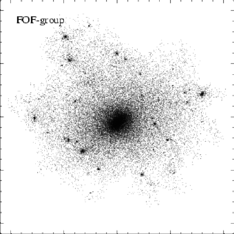
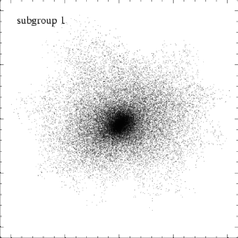
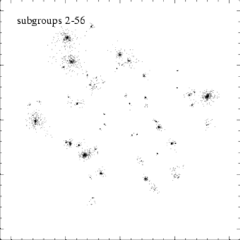
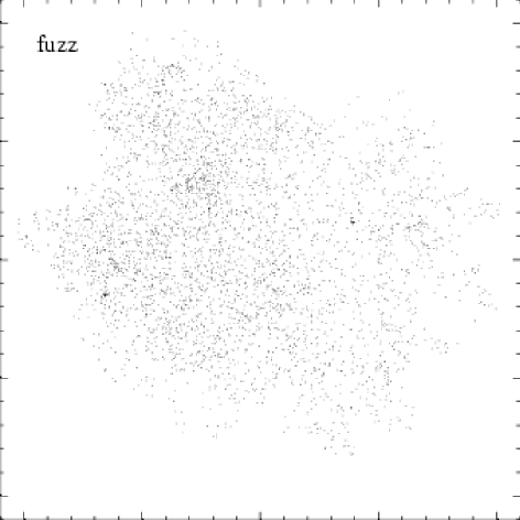
Figure 3: Example for a subhalo identification with SUBFIND. The top left panel shows a small FOF-group (44800 particles), identified at $z=0$ in the vicinity of the S2 cluster. SUBFIND identifies 56 subhaloes within this group, the largest one forms the background halo and is shown on the top right, while the other 55 subhaloes are plotted on a common panel on the lower left. In this example, the total mass in all the “true” subhaloes 2-56 is about 8% of the group mass. Particles not bound to any of the subhaloes form “fuzz”, and are displayed on the lower right. These particles primarily lie close to the outer edge of the group. Spatial coordinates are given in $\,h^{-1}{\rm kpc}$.

Note that it is unlikely that we lose any substructure by restricting the search to ordinary FOF-groups. FOF may accidentally link two structures, a case SUBFIND will be able to deal with, but we rarely expect FOF (with a linking length of $0.2$) to split a physical structure into two parts.

In SUBFIND, we begin by computing a local estimate of the density at the positions of all particles in the input group. This is done in the usual SPH-fashion, i.e. the local smoothing scale is set to the distance of the $N_{\rm dens}$ nearest neighbour, and the density is estimated by kernel interpolation over these neighbours. The particles may be viewed as tracers of the three-dimensional dark matter density field. We consider any locally overdense region within this field to be a substructure candidate. More specifically, we define such a region as being enclosed by an isodensity contour that traverses a saddle point. How can one find these regions? Imagine lowering a global density threshold slowly within the density field. For most of the time, isolated overdense regions will just grow in size as the threshold is lowered, except for the moments when two separate regions coalesce to form a common domain. Note that at these instances, the contours of two separate regions join at a saddle point. As a result the topology of the isodensity contour changes as well.

Our algorithm tries to identify all locally overdense regions by imitating such a lowering of a global density threshold. To this end, we sort the finite number of particles according to their density, and we ‘rebuild’ the particle distribution by adding them in the order of decreasing density. Whenever a new particle $i$ with density $\rho_{i}$ is considered, we find the $N_{\rm ngb}$ nearest neighbors within the full particle set. Within this set ${\cal A}_{i}$ of $N_{\rm ngb}$ particles, we also determine the subset of particles with density larger than $\rho_{i}$, and among them we select a set ${\cal B}_{i}$ containing the two closest particles. Note that this set may contain only one particle, or it may be empty. We now consider three cases:

1. The set ${\cal B}_{i}$ is empty, i.e. among the $N_{\rm ngb}$ neighbors is no particle that has a higher density than particle $i$. In this case, particle $i$ is considered to mark a local density maximum, and it starts growing a new subgroup around it.

2. If ${\cal B}_{i}$ contains a single particle, or two particles that are attached to the same subgroup, the particle $i$ is also attached to this subgroup.

3. ${\cal B}_{i}$ contains two particles that are currently attached to different subgroups. In this case, the particle $i$ is considered to be a saddle point, and the two subgroups labeled by the particles in ${\cal B}_{i}$ are registered as subhalo candidates. Afterwards, the particle $i$ is added by joining the two subgroups to form a single subgroup. Note that all subhalo candidates will be examined for self-boundedness later on in the algorithm.

Working through this scheme results in a list of subhalo candidates, which can be efficiently stored in a suitably arranged link-list structure. Note that a given particle can be member of several different subhalo candidates, and that the algorithm is in principle fully capable of detecting arbitrary levels of “subhaloes within subhaloes”.

Up to this point, the construction of subhalo candidates has been based on the spatial distribution of particles alone. A more physical definition of substructure is obtained by adding the requirement of self-boundedness. We therefore subject each subhalo candidate to an unbinding procedure to obtain the “true” substructure. To this end, we successively eliminate particles with positive total energy, until only bound particles remain. We perform the unbinding in physical coordinates, where we define the subhalo’s center as the position of the most bound particle, and the velocity center as the mean velocity of the particles in the group. We then obtain physical velocities with respect to this group center by adding the Hubble flow to the peculiar velocities. Finally, if more than a minimum number of $N_{\rm ngb}$ particles survive the unbinding, we refer to these particles as a subhalo.

An important issue remains of how one should deal with complications arising from the assignment of particles to several different subhalo candidates. This does not only occur if one deals with genuine “substructure within substructure”, but is actually quite typical for the algorithm. For example, imagine a large halo containing several small subhaloes. Whenever one of the small haloes ‘separates’ from the main halo, two subhalo candidates are generated according to case (iii) of the algorithm. Each time the larger of these groups describes the bulk of the main halo, which will thus appear several times as a subhalo candidate, although one would like to consider it only once as an independent physical structure.

We approach this issue by considering only the smaller subhalo candidate at each branch of the tree generated by the saddle points. This is based on the notion that we want to examine substructure within some larger object, and this ‘background’ object is expected to have larger mass than the actual substructure. In addition, we process the subhalo candidates in the inverse sequence as they have been generated, i.e. we work through the saddle points from low to high density. In this way, a smaller subhalo within a larger subhalo will always be processed later than its parent subhalo. As we consider the subhalo candidates in this order, each particle carries a label indicating the subhalo it was last detected to reside in. If in the process it is found to be contained also within a smaller subhalo, this label will be overwritten by the new subgroup identifier.

In this way, the complexity of our analysis is reduced by assigning each particle at most to one subhalo. We are still able to detect a hierarchy of small subhaloes within larger subhaloes, albeit at the expense of reducing the latter by the particles contained at deeper levels of the hierarchy. However, this usually does not affect the corresponding parent subhalo strongly, since the mass of any substructure within a larger group is usually small compared to that of the parent group. Nevertheless, it can happen that the extraction of subhaloes unbinds some additional particles from the parent subhalo. For this reason, we check all the disjoint subhaloes at the end of the process yet again for self-boundedness. Here, we also assign all particles not yet bound to any subhalo to the “background halo” of the group, which we define as the largest subhalo within the original FOF input group, and we check whether they are at least bound to this structure. If not, these particles represent ‘fuzz’, identified by FOF to belong to the group, but not (yet) gravitationally bound to it.

In summary, SUBFIND decomposes a given particle group into a set of disjoint self-bound subhaloes, each identified as a locally overdense region within the density field of the original structure. The algorithm is spatially fully adaptive, and it has only two free parameters, $N_{\rm dens}$ and $N_{\rm ngb}$. The latter of these parameters sets the desired mass resolution of structure identification, and we usually employ $N_{\rm ngb}=10$ for this purpose. The results are quite insensitive to the other parameter, the number $N_{\rm dens}$ of SPH smoothing neighbours, which we typically set to a value slightly larger than $N_{\rm ngb}$.

Finally, we note that any efficient practical implementation of the algorithm requires the use of hierarchical tree-data structures, and fast techniques to find nearest neighbours and gravitational potentials. For this purpose, we employ techniques borrowed from our tree-SPH code GADGET.

In Figure 3, we show a typical example of substructure identified using SUBFIND. We selected a small group from the periphery of the S2-cluster, at $z=0$, for this illustration. By eye, one can clearly spot substructure embedded in the FOF-group. The algorithm SUBFIND finds 56 subhaloes in this case. The largest one is the ‘background’ halo, shown in the top right panel of Fig. 3. It represents the backbone of the group, with all its small substructure removed. This substructure is made up of 55 subhaloes, which are plotted in a common panel on the lower left. While this example shows an isolated and well relaxed halo, we note that SUBFIND also performs well in cases where FOF links structures across feeble particle bridges, or when haloes are in the process of merging. In these cases, the algorithm reliably decomposes the FOF group into its constituent parts.

4.3 Subhaloes in the S1, S2, S3, and S4 clusters

Substructure within dark matter haloes is in itself a highly interesting subject that merits detailed investigation. What are the structural properties of subhaloes within haloes? What is their distribution of sizes and masses? What is their ultimate fate? Answers to these questions are highly relevant for a number of diverse topics such as galaxy formation, the stability of cold stellar disks embedded in dark haloes, or the weak lensing of galaxies in clusters (Geiger & Schneider 1998, 1999).

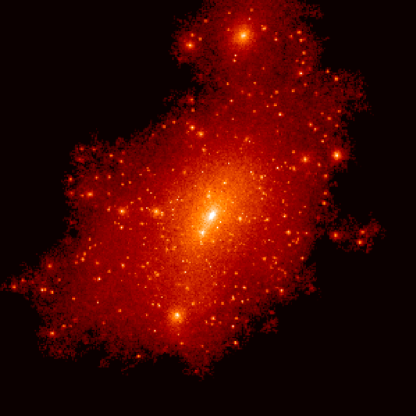
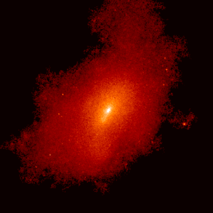
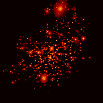
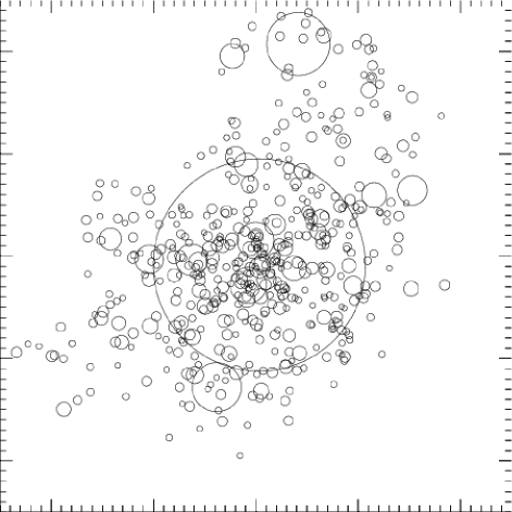
Figure 4: Substructure in the S2 cluster at $z=0$. The top left panel shows a color-coded projection of the FOF-group that contains the cluster. To highlight the substructure, particles have been given a weight proportional to the local dark matter density. In the top right panel we show the largest subhalo identified by SUBFIND, i.e. the background halo. The lower right shows the 495 other subhaloes identified in the object. Finally, on the lower right, we plot circles at the positions of each identified subhalo, with radius proportional to the third root of the particle number in the subhalo. Note that we actually found subhaloes within subhaloes in this example.

Tormen et al. (1998), Ghigna et al. (1998) and Klypin et al. (1999) have addressed some of these questions, and it will be interesting to supplement their work with results obtained from our new group-finding technique. However, such a study is beyond the scope of the present paper, where we focus on semi-analytic models for the galaxy population of the cluster. We therefore defer a detailed statistical analysis of substructure to future work, and just report the most basic properties of the subhaloes identified in the clusters at redshift $z=0$.

Figure 5: Subhalo mass functions in the four clusters S1, S2, S3 and S4 at redshift $z=0$. In the top panel, we plot the cumulative number $N(m)$ of subhaloes with masses larger than $m$. The short vertical lines mark the ends of the graphs for the simulations S1 (lowest resolution), S2, and S3 (second highest resolution). The agreement between the four simulations is quite good. This good agreement is also present in the differential mass function ${\rm d}N/{\rm d}m$, which we show in the lower panel.

Especially interesting is a comparison of the mass spectra of subhaloes detected in the four cluster simulations S1, S2, S3 and S4. In this sequence of simulations, the mass and force resolution increases substantially, which clearly leads to a larger number of resolved subhaloes: 118 subhaloes are detect in the final cluster of S1, 496 in S2, 1848 in S3, and 4667 in S4.

The increase in numerical resolution thus unveils an enormous richness of structure in the cluster. As an example, we show a plot of the substructure in the S2-cluster in Figure 4. Note that almost all of the additional substructure that becomes visible with still higher numerical resolution is in objects of smaller mass than the ones resolved in Figure 4. This is seen in a comparison of the cumulative and differential mass spectra, as shown in Figure 5. S1, S2 and S3 are actually well capable of resolving all the objects above their respective resolution limits. Even close to their resolution limits they predict the right abundance of subhaloes of a given mass.

4.4 Merging trees using substructure

We now describe our methods to construct merging trees that take the identified subhaloes into account. Note that SUBFIND classifies all particles of a given FOF-group either as lying in a bound subhalo, or as unbound. Any ordinary FOF-group lacking substructure will also appear in the list of subhaloes identified by SUBFIND, albeit only with its bound subset of particles. Since the requirement of self-boundedness is a reasonable physical condition for the definition of dark haloes, we therefore consider the list of haloes generated by SUBFIND as the ‘source list’ for our further analysis. Notice that we use the FOF-groups as convenient ‘containers’ to establish a simple two stage hierarchy of haloes. We define the largest subhalo in a given FOF-group as the main halo hosting the central galaxy. All other subhaloes found within the group will be considered to be substructure of this main halo.

In the following discussion, the term subhalo will refer to any self-bound structure identified by SUBFIND, even if it is just the self-bound part of an ordinary FOF-group that has no real substructure. In addition, we adopt the following definitions:

A subhalo $S_{\rm B}$ at redshift $z_{\rm B}$ is a progenitor of a subhalo $S_{\rm A}$ at redshift $z_{\rm A}<z_{\rm B}$, if more than half of the $N_{\rm link}$ most-bound particles of $S_{\rm B}$ end up in $S_{\rm A}$. This definition concentrates on the most-bound core of each structure, and we have found it to be very robust in tracing subhaloes between different output times. One can choose $N_{\rm link}$ as some fraction of the number of particles of subhalo $S_{\rm B}$, say all or half of them. However, such a condition may fail if $S_{\rm B}$ is deprived of its outer halo between two outputs, as it may occasionally happen when a structure of relatively large mass falls into a cluster. We have found that setting $N_{\rm link}=10$, equal to our lower particle limit for group identification, can satisfactorily treat even these cases. Note that our notion of ‘most-bound’ refers to the most negative binding energy. SUBFIND automatically stores each subhalo in the order of increasing binding energy to facilitate this kind of linking, i.e. the subhaloes are effectively stored from inside to outside.

We call a subhalo $S_{\rm B}$ at redshift $z_{\rm B}$ a progenitor of a FOF-group $G_{\rm A}$ at redshift $z_{\rm A}<z_{\rm B}$, if more than half of the particles of $S_{\rm B}$ are present in $G_{\rm A}$. We also call a FOF-group $G_{\rm B}$ a progenitor of a subhalo $S_{\rm A}$, if more than half of the particles of $S_{\rm A}$ are contained in $G_{\rm B}$. Note that in this latter condition we deliberately used the particles of $S_{\rm A}$ to define ‘membership’ in one of the FOF-group at higher redshift.

We expect that once a self-bound structure has formed, most of its mass will remain in bound structures in the future. However, occasionally it may happen that a group that was just barely above our specified minimum particle number at one output time falls below this limit at the next output time, for example because the group is evaporated by interactions with other material, or because of noise in the identification of groups with size close to our identification threshold. We call such groups volatile, and drop them from our analysis. More precisely: All FOF-groups without any bound subhalo are considered to be volatile and disregarded. In addition, if a subhalo is not progenitor to any other subhalo, and not progenitor to any non-volatile FOF-group, it is considered to be volatile too, and dropped from further analysis. Note that basically all subhaloes eliminated in this way have particle numbers very close to the detection threshold.

After the elimination of volatile subhaloes, we link subhaloes between pairs of successive simulation outputs. By construction, every subhalo may have several progenitors, but itself can only be progenitor for at most one other subhalo. In fact, due to the elimination of volatile subhaloes, a subhalo $S_{\rm B}$ will always be progenitor to another subhalo, or at least to a FOF-group $G_{\rm A}$. If only the latter is the case, we treat the subhalo $S_{\rm B}$ as a progenitor of the main halo within the FOF-group.

There remains then the important case that a subhalo $S_{\rm A}$ has no progenitor. If it also has no progenitor FOF-group, we call this subhalo a new galaxy, which is considered to have newly formed between the two output times. In the galaxy formation scheme, new galactic ‘seeds’ will be inserted into these subhaloes.

If however the subhalo $S_{\rm A}$ has no progenitor subhalo, but a progenitor FOF-group $G_{\rm B}$, it is likely that either the subhalo represents a chance fluctuation, or that it was overlooked in the identification process at the time $z_{\rm B}$. In the latter case the corresponding structure will have been merged with the main halo, so we drop these subhaloes. Their absolute number and the total mass contained in them is always very small.

In summary, the above identification scheme allows a detailed tracing of the dark matter merging history tree, from the past to the present. In particular, the scheme is able to deal with haloes that pop into existence, that grow in size by accreting additional background particles, that merge with other haloes of comparable size and lose their identity, or that fall into a larger halo without being destroyed completely. The latter case is particularly interesting, since we expect that a subhalo can survive for some time within the larger structure. However, its mass can be reduced by tidal stripping, an effect that can eventually completely dissolve the structure.

4.5 Inclusion of subhaloes in semi-analytic models

One of the questions we want to address in this study is how the inclusion of subhaloes changes the results of semi-analytic models. In order to highlight such changes we will modify the ‘standard’ scheme, which is based on the work of KCDW, in a minimum fashion when subhaloes are included.

Figure 6: The I-band Tully-Fisher relation for Sb/Sc galaxies in the S2 simulation. The two panels on top have been obtained with the subhalo-scheme using ejection and retention feedback, respectively, while the two panels on the bottom show the equivalent plots using the standard-scheme of KCDW. The galaxies have been selected as central galaxies of uncontaminated haloes in the periphery of the cluster. The solid line represents the recent measurement by Giovanelli et al. (1997).

Note that a large variety of semi-analytic “recipes” are conceivable, and that some of the results can depend sensitively on the specific set of assumptions made, as has been recently highlighted by KCDW. Semi-analytic models thus cannot eliminate uncertainties arising from poorly constrained physics. However, they are ideal tools to explore the relative importance of various model ingredients, and hence to constrain their relevance for observed trends in observational properties.

We now describe the changes in our semi-analytic methodology when subhaloes are included. From here on, we will refer to the formalism of KCDW, which only works with FOF groups, as the ‘standard’-scheme, and to the analysis that includes substructure as the ‘subhalo’-scheme. We note that the word ‘standard’ is not meant to imply that the corresponding procedure has (yet) the status of a well-established, widely used method in the field – it is just used to refer to the methodology recently developed by KCDW.

Our most important change concerns the definition of the galaxy population at each output time. We define the largest subhalo in a FOF-group to host the central galaxy of the group, and this galaxy’s position is given by the most-bound particle in that subhalo. All gas that cools within a FOF-group is funneled exclusively to the central galaxy. This definition of ‘central galaxy’ thus corresponds to the one adopted in the standard analysis.

For the population of galaxies orbiting within a halo, however, we distinguish between halo-galaxies and satellite galaxies. Here we have coined yet another term; ‘halo-galaxies’ are attached to the most bound particle of the remaining subhaloes in the FOF-group. These halo-galaxies were proper central galaxies in the past, until their halo fell into a larger structure. The core of this halo is, however, still intact, and thus allows an accurate determination of the position of the halo-galaxy within the group. These halo-galaxies may still be viewed as ‘central galaxies’ of their respective subhaloes, but they are no longer fed by a cooling flow since their subhalo is not the largest within the FOF group.

Finally, when two (or more) subhaloes merge, the halo-galaxy of the smaller subhalo becomes a satellite of the remnant subhalo. These satellites are treated as in the standard analysis. Their position is tagged by the most-bound particle identified at the last time they were still a halo-galaxy, and they are assumed to merge on a dynamical friction timescale with the halo-galaxy of the new subhalo they now reside in. We need to introduce such satellites in the subhalo-scheme in order to account for actual mergers between subhaloes, and also because of the finite numerical resolution of our simulations, which limits our ability to track the orbits of subhaloes once their mass has fallen below our resolution limit. It also allows us to make direct contact with the standard-scheme in the limit of poor resolution. Note that the class of halo-galaxies is absent in the standard analysis, where all of these galaxies are treated as satellites.

Table 2: Numerical parameters adopted for our semi-analytic models. $\alpha$ is the star formation efficiency, $\epsilon$ the efficiency of feedback by supernovae, and $f_{\rm b}$ the baryon fraction.

Model	$\alpha$	$\epsilon$	$f_{\rm b}$
ejection	0.05	0.10	0.15
retention	0.05	0.15	0.15

In the subhalo scheme, we define the virial mass $M_{\rm vir}$ of a subhalo simply as the total mass of its particles. For the background subhalo, we then define virial radius and virial velocity by assuming that the halo has an overdensity 200 with respect to the critical density. For other subhaloes we keep the virial velocity and the halo’s dynamical time at the values they had just before infall.

5 Results

5.1 Tully-Fisher relation

We use the velocity-based I-band Tully-Fisher relation

$$M_{I}-5\log h=-21.00-7.68\,(\log W-2.5)$$ (14)

of Giovanelli et al. (1997), and the requirement of a gas mass of $\sim 8\times 10^{9}\,h^{-1}{\rm M}_{\odot}$ in ‘Milky-Way’ haloes, to normalize our models. We consider two variants for the implementation of feedback, the ‘ejection’ model, where gas is blown out of small haloes, and the ‘retention’ model, where reheated gas is always kept within the halo.

In Figure 6, we show the best-fit Tully-Fisher relations obtained for these two models, applied to the S2-cluster using the ‘subhalo’ and the ‘standard’-schemes. In the plots, we only considered central galaxies of haloes that are peripheral to the cluster, but that are not contaminated by heavier boundary particles. We also applied a morphological cut, $1.2\leq M_{\rm bulge}-M_{\rm total}\leq 2.5$, approximately selecting Sb/Sc galaxies. In Table 2, we list the model parameters thus obtained. In the following, we will use the same set of parameter values also for our other cluster simulations, and for the ‘standard’ semi-analytic scheme.

The Tully-Fisher relations we obtain exhibit remarkably small scatter. This is partly a result of the tight coupling we assumed between the sizes and circular velocities of the disks of spiral galaxies and the masses of their dark haloes. Note that additional scatter can be expected from the distribution of spin parameters of dark haloes, which gives rise to variations of the disk sizes associated with a halo of a given mass (Mo et al. 1998).

The ejection model fits the slope of the observed TF-relation relatively easily. However, the retention model is less effective in suppressing star formation in low mass haloes. For the same value of $\epsilon$, the retention scheme therefore produces a shallower Tully-Fisher relation than the ejection model. As a result, a larger value of $\epsilon$ is needed to bring the retention model in agreement with the observed steepness of the TF-relation. This strong feedback reduces the overall brightness somewhat, an effect that could be easily compensated for by slightly larger values for $\alpha$ or $f_{\rm b}$. Note that a feedback efficiency of $\epsilon=0.1$ means that feedback will be quite efficient in haloes of virial velocity below $V_{\rm SN}=183\,{\rm km}\,{\rm s}^{-1}(\epsilon/0.1)^{1/2}$. In such haloes, one will have $\Delta M_{\rm reheat}\geq\Delta M_{\star}$, i.e. the mass of reheated gas exceeds that of newly formed stars.

Figure 7: The four panels compare the I-band Tully-Fisher relations obtained for the S1, S2, S3, and S4 simulations using the subhalo-scheme and ejection feedback. The models with retention feedback, and the models using the ‘standard’ scheme, are able to match the observed Tully-Fisher relation about equally well.

It is also interesting to compare the Tully-Fisher relations obtained for the different cluster simulations (see Figure 7). For the sake of brevity, we restrict the comparison to the subhalo scheme with ejection feedback. In general, there is good agreement between the two variants of semi-analytic modeling, and between the four different simulations, despite their large differences in numerical resolution. For the same choice of free parameters, the slopes and zero-points of the Tully-Fisher relations agree quite well. There may be a weak trend towards fainter zero-points in the sequence S1 to S4. Note that the scatter in the Tully-Fisher relation increases at low velocity widths because feedback has a stronger effect on galaxies with low $V_{\rm c}$. A similar trend in the observed scatter has been found by Matthews et al. (1998).

5.2 Cluster luminosity function

In Figure 8, we show the B-band luminosity function of the S2-cluster obtained with the new ‘subhalo’ methodology, and we compare it to the result of the ‘standard’ semi-analytic recipe of KCDW. We plot the number of cluster-galaxies in bins of size 0.5 mag, and we fit Schechter functions to the counts. The standard prescription results in a relatively steep slope of $-1.31$ at the faint-end, and the “knee” of the Schechter function is not well defined. This is just another reincarnation of a well-known problem in many previous semi-analytic studies, which predicted too many galaxies both at the faint and the bright end of the the luminosity function, i.e. the shape was not curved enough. These deficiencies can be partly cured by invoking additional physics like dust obscuration, or by employing models with very strong feedback processes. However, most semi-analytic studies have not been successful in simultaneously achieving good agreement with the Tully-Fisher relation and the luminosity function.

Figure 8: The histograms show the B-band cluster luminosity function obtained for the S2 simulation using the subhalo scheme (left) and the standard scheme (right). We here show results for the ejection feedback, and note that the results for the retention model are very similar. The symbols and error bars give the composite luminosity function found by Trentham (1998) as a weighted mean of 9 clusters, all having luminosity functions that are individually consistent with the composite one. Note that we adjusted the vertical normalization of the composite function (which is arbitrary) to obtain a good fit to the total luminosity of the cluster. The solid lines are Schechter function fits to the histograms of bin-size 0.5 mag. For the subhalo model, the faint end slope is $\alpha=-1.21$, and the turn-off is at $M_{\star}\simeq-21.8$. The standard scheme results in a steeper slope of $\alpha=-1.31$, and the characteristic magnitude is not well defined. Note that the standard model produces a central galaxy of magnitude -23.9, which appears too bright even comparing to the brightest cD galaxies.

Figure 9: The B-band cluster luminosity functions obtained for the S1, S2, S3, and S4 simulations using the subhalo scheme and ejection feedback. The solid lines are three-parameter Schechter function fits to the histograms of bin-size 0.5 mag. The formal values for faint-end slope and cut-off of these fits are: S1 ($\alpha=-1.22$, $M_{\star}=-22.8$), S2 ($\alpha=-1.21$, $M_{\star}=-21.8$), S3 ($\alpha=-1.21$, $M_{\star}=-21.7$), and S4 ($\alpha=-1.24$, $M_{\star}=-22.0$). Symbols with error bars give the composite observational result by Trentham (1998). Dashed histograms give the luminosity functions of subhalo galaxies alone, i.e. galaxies that still have an associated dark matter subhalo.

Compared to the field, the luminosity functions of clusters tend to be considerably steeper, and a slope of $-1.31$ can be accommodated with existing data. However, the standard-scheme also produces a brightest cluster galaxy with luminosity in excess of most normal cD galaxies. For example, in the S2 cluster, the standard-scheme produces a central galaxy with B-magnitude $-23.9$.

In contrast, the luminosity function obtained with the subhalo formalism has a more curved shape. There are more $L_{\star}$-galaxies, resulting in a flatter faint-end slope of $\alpha=-1.21$, and in a more pronounced “knee”, which is much better fit with a Schechter function. In addition, the luminosity of the central galaxy is reduced. The overall shape of the resulting luminosity function is in reasonably good agreement with observed cluster luminosity functions, as shown by a comparison with the composite luminosity function of Trentham (1998), which is indicated with symbols in Figure 8.

What causes this difference between the subhalo-scheme and the standard scheme? Note that the excessive brightness of the central galaxy in the latter model is unlikely to be caused by an overcooling problem. We have already cut-off the cooling flow for central galaxies in haloes with a virial velocity larger than $350\,{\rm km}\,{\rm s}^{-1}$. Furthermore, the cooling model was essentially the same for both schemes, which is also reflected in their similar overall mass-to-light ratios.

The most important difference between the ‘standard’ semi-analytic scheme and the ‘subhalo’-methodology is the explicit tracking of subhaloes, which allows more faithful modeling of the actual merging rate in any given halo. Recall that one critical assumption in the study of KCDW is that the time of survival of a satellite can be estimated using a simple dynamical-friction formula. However, this description is crude and the excessive brightness of the central galaxies may result from an overestimate of the overall merging rate, or from merging the ‘wrong’ galaxies. Recall that a second important assumption of KCDW has been that the position of a satellite galaxy can be traced by a single particle identified as the most-bound particle of the satellite’s halo just before it was accreted by a larger system.

Before we investigate these assumptions in more detail, we plot in Figure 9 the cluster luminosity functions for the S1, S2, S3 and S4 clusters, obtained with the subhalo scheme and ejection feedback. All four simulations produce luminosity functions which can be well described by Schechter functions with a well defined cut-off. Their shape is in fact quite close to the obervational result by Trentham (1998), shown with symbols in each of the four panels. The vertical normalization of his composite observational result is arbitrary, and we have set it to match the total luminosity of our cluster(s). It is however the same in all four panels. Agreement of the luminosity functions between the four simulations is quite good, with the simulations of higher mass resolution able to probe the luminosity function to ever fainter magnitudes. It is interesting to note that as the resolution of the simulations increases, a larger and larger fraction of the galaxies have their own dark matter halo (this is indicated by a dashed line in the plot). In S4, almost all bright galaxies still have an associated dark matter substructure, and it seems likely that in still larger numerical simulations the correspondence would be perfect.

However, when comparing the luminosity functions with each other, there is a trend of decreasing brightness of the first ranked cluster galaxies with increasing resolution. We think that this is a reflection of inaccuracies in estimates of merging timescales, which become more serious in simulations with lower resolution. This effect may also be responsible for the weak trend in the zero-points of the Tully-Fisher relations (Figure 7).

We now test whether this problem is responsible for the difference between the subhalo scheme and the standard formalism. To this end we try to answer the question: How many of the galaxies present in subhaloes of S2 at $z=0$ are prematurely merged with the center in the standard scheme?

To do this, we follow each subhalo of the cluster back in time along its merging history until it is a main halo itself for the first time. The corresponding FOF-halo will host a central galaxy in the standard scheme, and the descendant of this galaxy at $z=0$ should directly correspond to the galaxy of the originally selected subhalo.

Among the 494 subhaloes identified in the S2-cluster at $z=0$, we find in this way that 39 of them do not have a directly corresponding satellite galaxy in the ‘standard’-formalism. The satellites that should correspond to these 39 subhaloes have prematurely disappeared by merging processes with the central galaxy, because their merging timescales have been underestimated. Note that the total number of mergers with the central galaxy in the standard scheme is 116, while this number is 132 in the subhalo formalism. This suggests that the overall rate of mergers is not too high in the standard scheme. However, in the standard scheme the central galaxy accretes 24 galaxies with stellar masses of more than $10^{10}\,h^{-1}{\rm M}_{\odot}$, among them 8 galaxies with stellar masses larger than $10^{11}\,h^{-1}{\rm M}_{\odot}$. On the other hand, in the subhalo formalism there is only 1 merger involving more than $10^{11}\,h^{-1}{\rm M}_{\odot}$, and 11 with more than $10^{10}\,h^{-1}{\rm M}_{\odot}$. This means that a larger number of very bright galaxies is merged with the central galaxy in the standard scheme. We also note that the galaxies in the 39 subhaloes that appear to have been merged prematurely in the standard scheme tend to be quite bright. If we take the results for the subhalo-model and add the luminosities of the corresponding halo-galaxies to that of the central galaxy, its brightness increases from -21.9 to -24.1 mag, quite close to the -23.9 obtained in the standard-scheme. It thus appears that the excessive brightness of the central cluster galaxy in the standard scheme is mainly caused by an underestimate of the merging timescales for some fraction of the bright galaxies.

We have also tested how well the position of subhaloes corresponds to those of single particles used to track satellites in the standard scheme. We find that a fraction of 86.8% of the subhaloes in S2 still contain the most-bound particle that is used in the standard-scheme to track the position of the satellite. This number is 86.6% in S1, 82.2% in the S3 cluster, and 76.3% in the S4 cluster. Note that these numbers have been computed for all the subhalos in each of the simulations. To the mass resolution limit of the S1 cluster, the corresponding success rates are 93.6%, 89.4% and 96.8% in S2, S3, and S4, respectively. Using just a single particle identified at a time before a structure was accreted onto the cluster can thus provide a good estimate of the subhalo’s position within the cluster halo at later times.

Figure 10: Cumulative number of galaxies in the cluster as a function of radial distance to the cluster center. In the top panel, we count all galaxies with $M_{\rm B}<-16$, binned into three classes of different Hubble type. In the bottom panel, only the bright galaxies with $M_{\rm B}<-18$ are shown. In both panels, the shape of the cumulative dark matter mass distribution is indicated by a thin solid line, for comparison. The results shown are for the S4 cluster using ejection feedback.

It thus seems clear that the difference between the luminosity functions of the standard and subhalo schemes is largely caused by differences in the assumed merger timescales of galaxies that fall into the cluster. Recall that for the choices we adopted in equation (9), the dynamical friction formula is essentially the current dynamical time of virialized haloes times the mass ratio of the halo and its infalling satellite. Large estimates of merger timescales arise when the mass of the satellite is much smaller than that of the halo. In fact, small satellites will typically have merger timescales that are much larger than a Hubble time, while large infalling haloes are predicted to merge with the central galaxy quickly. As a result, the standard scheme appears to merge some of the associated bright galaxies ‘too early’, making the central galaxy excessively bright. In the subhalo scheme, these galaxies are still around and populate the ‘knee’ of the luminosity function. Note however that the dynamical friction estimate in the simple form applied here does not include the effects of tidal truncation and disruption, which presumably act to reduce the lifetime of small satellites, but may increase the lifetime of infalling massive satellites. In fact, the results of Tormen et al. (1998) indicate that the dependence of the merger timescale on the mass ratio, measured just before the satellite falls in, is weaker than linear.

Presently it is unclear whether an improved parameterization of the merger timescales in the standard scheme can produce results as good as those obtained by explicitly following the subhaloes. However, a more detailed investigation of the probability distribution of actual merging timescales may well make this possible, and offers the prospect of implementing more accurate satellite merging in the ‘standard’ semi-analytic scheme, even when simulations with relatively poor resolution are used.

5.3 Morphology density relation

Dressler (1980) has shown that the relative frequency of elliptical galaxies is higher in denser environments. In particular, in the cores of clusters, spirals are quite rare, while they are the dominant type in the field, and in the Universe as a whole. Whitmore et al. (1993) have argued that this morphology-density relation reflects a more fundamental morphology-clustercentric relation; the correlation between morphology and clustercentric separation seems tighter than that between morphology and projected density. This assertion is still controversial.

Figure 11: Morphological mix of galaxies as a function of clustercentric radius. From top to bottom, the symbols in the three panels show the relative fraction of elliptical, S0, and spiral galaxies in spherical shells around the cluster center, with error bars given by counting statistics. Filled symbols are for galaxies brighter than $M_{\rm B}=-17$, and hollow symbols for a sample selected at $M_{\rm B}=-18.5$. Filled circles show the observational results of Whitmore et al. (1993). Note that we here follow these authors in letting the radius decrease to the right, i.e. the cluster center is found on the right side of the diagrams. The results shown here are for the S2 and S4 simulations, using the subhalo modeling with ejection feedback. Results for the other two simulations are similar.

In Figure 10, we show the cumulative number of galaxies of different Hubble type as a function of distance from the cluster center. The top panel gives all the galaxies with $M_{\rm B}<-16$, while in the bottom panel we just show the bright galaxies with $M_{\rm B}<-18$. From the cumulative distribution it can be inferred that the three-dimensional density profile of the ellipticals has a steeper slope than that of the spirals, i.e. they are more concentrated towards the center. Note that the thin solid line gives the shape of the cumulative dark matter profile for comparison. It is also interesting to note that the bright galaxies in the center are primarily ellipticals, while their mean Hubble type shifts to later types towards the outskirts of the cluster.

These trends in the morphological mix of galaxies can be more clearly seen in Figure 11, where we show the morphology-clustercentric relations obtained for the S2 and S4-clusters, using the subhalo-scheme with ejection feedback. Note that the fraction of elliptical galaxies strongly rises towards the center of the cluster, while that of the spirals declines accordingly. The quantitative strength of these trends is in reasonable agreement with the results of Whitmore et al. (1993), although there are small differences in detail. For the classification of galaxies, we applied cuts in $T$-space that count galaxies with $0<T<5$ as S0’s, and lower (higher) types as ellipticals (spirals), respectively. The resulting relative populations of galaxies of different types are consistent with the observed morphological mix, and largely independent of the magnitude cut-off for the sample. Note however that in the standard observational classification a slightly different cut in $T$-space is used for S0’s. This may just reflect the difficulty to unambiguously define the transitional type S0 in our coarse morphological classification scheme, or it may mean that additional physical processes are at work to create real S0 galaxies.

Recall that our morphological modeling is solely based on the merging history of galaxies. Ellipticals are formed in major mergers, which occur more frequently in higher density environments. This simple model suffices to establish a pronounced morphology density relation. This shows that the morphology density relation is built-in at a very fundamental level in hierarchical theories of galaxy formation.

In passing we note that in the standard recipe, where satellites are just traced by single particles once they have fallen into a larger halo, the morphology-clustercentric relation is also present, although it is not quite so well defined. The stronger clustering of early type galaxies was also found by KCDW, Diaferio et al. (1999) and more recently by Diaferio et al. (2000). Using techniqes somewhat similar to ours, Okamoto & Nagashima (2000) also found a morphology-density relation. All these papers argued that additional processes are required to understand the S0 population.

Figure 11 also shows that the fraction of S0’s in our cluster shows a weaker dependence on cluster-centric distance than the observations. This also suggests that S0’s experience additional processes in clusters that are not included in our analysis. For example, disk galaxies orbiting in a cluster experience high-speed encounters with other galaxies. Together with global cluster tides this can drive a morphological evolution towards spheroids, a process termed galaxy harassment (Moore et al. 1996, 1998). It has been suggested that the spiral galaxies seen abundantly in clusters at moderate redshift are harassed and slowly transformed to S0’s at the present time. Such an effect might explain our deficit of S0 galaxies inside the cluster.

5.4 Cluster mass-to-light ratio

The observed mass-to-light ratios of clusters of galaxies are known to be much larger than those of individual galaxies, and this fact has been recognized early on as strong evidence for the existence of large amounts of dark matter in clusters. Typical measured values for the cluster mass-to-light range from $\Upsilon_{B}=200\,h\,\Upsilon_{\odot}$ to $\Upsilon_{B}=400\,h\,\Upsilon_{\odot}$ in the B-band. For the Coma cluster, Kent & Gunn (1982) measured $\Upsilon_{B}=360\,h\,\Upsilon_{\odot}$, while X-ray data seem to point to a lower value. For example, Cowie et al. (1987) inferred a mass-to-visual-light ratio for Coma as low as $\Upsilon_{V}=180\,h\,\Upsilon_{\odot}$.

Figure 12: $B$-band mass-to-light ratio of halo galaxies as a function of distance to the cluster center (small symbols), expressed in units of the mass-to-light ratio of the cluster as a whole. For the masses of the galaxies we here simply took the dark matter masses of their corresponding subhaloes. The large symbols give the median mass-to-light ratios in radial bins around the cluster center. There is a clear trend of decreasing $M/L$ towards the cluster center, largely reflecting the mass loss of subhaloes due to tidal truncation. Note however that early type galaxies appear to have a systematically lower mass-to-light ratio than late types.

The galaxy population constructed for the S4 cluster using the subhalo model has a total magnitude of $M_{B}=-26.04$. For its total mass of $8.36\times 10^{14}\,h^{-1}{\rm M}_{\odot}$, the cluster mass-to-light ratio is thus $\Upsilon_{B}=420\,h\,\Upsilon_{\odot}$. In the V-band, we obtain $M_{V}=-26.97$ and $\Upsilon_{V}=324\,h\,\Upsilon_{\odot}$. These mass-to-light ratios fall on the high side compared to the mean of observational results, although there are also measurements that are as large, or larger, as our values. For example, Kent & Gunn (1983) obtained $\Upsilon_{V}=600\,h\,\Upsilon_{\odot}$ for the Perseus cluster.

Small changes of the model parameters can, however, enhance the overall brightness of the cluster, and thus reduce the mass-to-light ratios to a desired value. One simple possibility is to change the conversion factor between the virial velocity and the circular velocity. If the circular velocity of a disk in a dark matter halo of given virial velocity is on average 15% larger than we assumed, the normalization to the Giovanelli et al. (1997) Tully-Fisher relation results in an overall increase in brightness of 0.5 mag, and a corresponding reduction of the mass-to-light ratio to 63% of its old value.

Dust obscuration can account for effects of similar size. It is quite likely that the observed average brightness of galaxies in the Giovanelli et al. (1997) sample is somewhat reduced by dust, even though the I-band is less affected by dust than bluer wavelengths. Since we do not correct for dust extinction in this work, our fit to the observed Tully-Fisher relation is expected to underestimate the stellar masses of these spirals. Correcting this would produce larger stellar masses for all galaxies at the present epoch and consequently lower mass-to-light ratios for the cluster.

We may also ask whether we detect systematic variations of the mass-to-light ratio of subhalo galaxies as a function of their position in the cluster. In Figure 12 we show the $B$-band mass-to-light ratio of halo galaxies as a function of radial distance to the cluster center. Here we took the dark matter masses of the corresponding subhaloes to compute $M/L$ ratios. The clear trend of decreasing $M/L$ towards the cluster center is caused primarily by mass loss through tidal truncation. However, for a given distance from the cluster center, there is also a systematic variation of mass-to-light ratio with morphological type. At each luminosity, early type galaxies tend to have lower mass halos than late types, reflecting their earlier incorporation and more effective stripping within the cluster. All the galaxies have mass-to-light ratios substantially smaller than the cluster as a whole.

Figure 13: Faber Jackson relations for cluster ellipticals (circles) and field/group ellipticals (filled stars). We here plot the $B$-band luminosity of subhalo-galaxies versus an estimate of the one-dimensional stellar velocity dispersion. The latter was taken to be $0.9/\sqrt{3}$ times the measured 3D-velocity dispersion of the galaxies’ dark matter subhalo identified in the simulation. The factor $1/\sqrt{3}$ converts from 3D to line-of-sight velocity dispersion, and the factor $0.9$ is needed to bring the zeropoint in agreement with the observed correlation. The obervational Faber-Jackson relation is shown as a solid line, and is adopted from the fit of Bender et al. (1996) to data for Coma and Virgo ellipticals.

5.5 Faber-Jackson relation

For elliptical galaxies, there is a well-known scaling relation between luminosity and central velocity dispersion, the so-called Faber-Jackson relation. In our formalism, we explicitly follow dark matter subhaloes that orbit inside larger group- or cluster-sized haloes. While the mass of these subhaloes decreases strongly over time by tidal truncation, their velocity dispersion remains relatively stable until they finally disrupt. Thus the velocity dispersion of a heavily truncated subhalo still reflects that of the original halo just before it fell into the cluster. It is plausible that the stellar velocity dispersions of elliptical galaxies correlate with the dark matter dispersions of their haloes (Rix et al. 1997). We may thus hope to find a Faber-Jackson-like relation if we plot the luminosity of our elliptical galaxies aginst the dark-matter velocity dispersion of their surrounding (sub)haloes.

In Figure 13 we show the resulting $B$-band Faber-Jackson relation for the S2 and S4 simulations. We here converted the measured 3D velocity dispersions of the dark matter of the subhalos to 1D dispersions, and we multiplied the resulting values by a factor $0.9$ to obtain an estimated stellar velocity dispersion. It is remarkable that the zeropoint, slope and scatter are consistent with the observed relation for cluster ellipticals, which is here adopted from Bender et al. (1996) for the Virgo and Coma clusters and drawn as a solid line. It is reassuring that the kinematics of the dark matter substructure has indeed the right properties to explain the Faber-Jackson relation. Note that some of the bright elliptical galaxies in this plot have heavily stripped subhaloes of relatively small mass, but the dark matter velocity dispersion of the residual subhalo is still large enough to put them at about the right place according to the Faber-Jackson relation.

5.6 Luminosity segregation

We have already seen that inside the cluster the number distribution of luminous elliptical and spiral galaxies does not follow the mass distribution of the dark matter. Does this also hold for the total light emitted by the cluster galaxies? In Figure 14, we show the cumulative luminosity profile of the cluster, and compare it to the dark matter mass profile. The luminosity profile is shallower than that of the mass, showing that the light is actually more concentrated than the mass, or phrased differently, the cumulative mass-to-light ratio decreases towards the cluster center. Note that the ‘steps’ in the light profile are caused by the finite number of galaxies and our assumption that they emit as point sources.

A related question is that of luminosity segregation, i.e. are more luminous galaxies more strongly concentrated than less luminous ones? Note that clustering strength is a strong function of circular velocity in CDM models (White et al. 1987), so some form of luminosity segregation should perhaps be expected. Since early-type galaxies tend to be brighter than late-type galaxies, luminosity segregation may also be seen as a consequence of the morphology density relation. However, it is then not so clear which of these two correlations is more fundamental. In fact, they might have a common origin in the local dynamics of the cluster core with its frequent mergers.

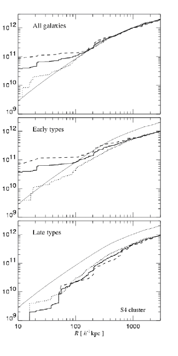
Figure 14: Luminosity segregation in the cluster S4. We here show the cumulative luminosity profile of $B$-band light of cluster galaxies (thick solid lines), and compare it to the cumulative dark matter mass profile (thin sold lines). The latter has been scaled by the overall mass-to-light ratio of the cluster to put the curves in the three panels on a common scale. While the top panel shows all the galaxies, we have devided them by morphological type into two equally luminous groups in the middle and bottom panels. In each panel, we further split the galaxies into a luminous (dashed lines) and a faint (dotted lines) group such that each of the groups produces just half of the total luminosity in the panel. Finally, we shifted the total luminosity profile in each panel by a factor of two to align the curves at the virial radius.

Figure 15: One-point velocity dispersion of galaxies (filled circles) brighter than $M_{B}=-17$ as a function of distance to the cluster center. The velocity dispersion of the dark matter is given by the solid lines in the four panels. The error bars mark the 68 per cent confidence intervals based on counting statistics. We have further split up the galaxies into a blue and a red sample of equal size, based on their $B-V$ color. The blue galaxies are shown as triangles, the red ones as boxes. Note that there are no very blue galaxies near the cluster center, hence triangular symbols are absent at small radii.

Observational evidence for luminosity segregation is still relatively sparse and controversial, primarily because of the difficulty in obtaining sufficiently large samples of faint cluster galaxies. Kashikawa et al. (1998) have recently studied the dependence of luminosity segregation on morphological type in the Coma cluster. In order to disentangle luminosity segregation from the morphology-density relations it is critical to understand whether it occurs within a given morphological type. Kashikawa et al. (1998) found that galaxies with high central concentration (early types) show signs of luminosity segregation, while galaxies of low central concentration (late types) do not exhibit any strong segregation.

In the two bottom panels of Figure 14, we investigate this issue for our cluster galaxies. We have divided the galaxies into early and late types, and we split each of the groups into a high and a low luminosity sample, such that the total luminosity in each group was divided into two equal parts. Interestingly, only the light of the bright elliptical galaxies is more concentrated than the mass of the cluster, while the low luminosity early types, and the spiral galaxies are distributed like the mass. We thus find evidence for luminosity segregation of early type galaxies. This is in agreement with the findings of Kashikawa et al. (1998). Notice however that Diaferio et al. (2000) found no clear evidence of luminosity segregation in their analysis of the GIF simulations.

5.7 Velocity dispersion of galaxies

One common technique to estimate masses of real clusters of galaxies is based on the virial theorem, requiring measurements of the line-of-sight velocity dispersion and of the projected separations of galaxies (Heisler et al. 1985). However, the accuracy of this technique can be compromised if cluster galaxies are biased tracers of the dark matter velocity distribution. Such systematic differences in the velocity fields will usually give rise to errors in the mass estimates of clusters. In fact, there have been controversial claims in the literature whether such a bias exists, and whether it is positive or negative. Since there is currently no consensus on this issue, we briefly address it here. In the following, we will focus on the one-point velocity bias, defined as the ratio $b_{v}=\sigma_{\rm gal}/\sigma_{\rm DM}$ of galaxy and dark matter velocity dispersions. We will refer to values of $b_{v}$ greater (less) than one as positive (negative) velocity bias.

In the early simulation work of Carlberg (1994) and Frenk et al. (1996), a negative velocity bias of up to 20-30% was reported. However, using the ‘standard’ scheme of semi-analytic modeling applied to the GIF-simulations, Diaferio et al. (1999, 2000) found a positive velocity bias in the outskirts of clusters, a result which can be explained as being due to the recent infall of star-forming blue galaxies.

Recent numerical studies with sufficient resolution to resolve substructure have led to somewhat conflicting results. Colin et al. (2000) found a substantial positive velocity bias, except perhaps in the innermost region of their cluster. A similar result, albeit of weaker strength, was obtained by Okamoto & Habe (1999). On the other hand, Ghigna et al. (1998) did not find any significant velocity bias in their analysis of cluster subhaloes. Similarly, Klypin et al. (1999) found no velocity bias on cluster mass scales, but a significant anti-bias for small groups of galaxies. In a more detailed analysis of this issue, Ghigna et al. (1999) recently reported a small positive velocity bias for subhaloes in the innermost region of their clusters, although the overall signal was considerably smaller than that found by Colin et al. (2000).

In light of this theoretical uncertainty, it is interesting to examine the velocity bias of our cluster simulations. In Figure 15, we plot the velocity dispersion of our model galaxies in the clusters S1-S4 as a function of radius. We used logarithmic bins and computed 68%-confidence intervals under the assumption that the galaxies in each bin are drawn from an underlying Gaussian velocity distribution. In this case, the estimated dispersions are expected to follow $\chi^{2}_{n-1}$ distributions, where $n$ is the number of galaxies in each bin.

Upon comparison with the dark matter velocity dispersion (solid lines) it is seen that we detect evidence for a small negative velocity bias in the central region of the cluster. The significance of this result is small for a single bin, but adjacent bins are independent here, and ‘noise’ between the four realizations is also uncorrelated, giving rise to a quite significant finding when the individual results are combined. We thus conclude that our models show evidence for a negative velocity bias in the innermost $\sim 300\,h^{-1}{\rm kpc}$ of the cluster, while further outside, velocity bias appears to be small, if present at all. Such a lower velocity dispersion in the center appears to be consistent with a number of observational studies (e.g. Biviano et al. 1992; Adami et al. 1998) that have found systematically smaller velocities for the brightest galaxies in the cores of clusters, although the observational evidence for this has not so far been fully convincing.

In Figure 15, we have also split up the galaxies into a blue and a red sample according to their $B-V$ color. Interestingly, it is seen that the blue galaxy sample shows larger velocity dispersions in the radial range $300-1000\,h^{-1}{\rm kpc}$. This is in agreement with the findings of Diaferio et al. (1999, 2000). Since these galaxies experienced relatively recent star formation, they have mostly just fallen into the cluster. As a result their orbits have systematically larger apocentres than those of red galaxies in the same region of the cluster. Note that if one selects the most massive subhaloes, one also obtains a population that has just fallen into the cluster and is biased towards its outskirts. This may explain why studies focusing on subhaloes have reported signs of positive velocity bias (Colin et al. 2000).

5.8 $B-V$ color distribution

Figure 16: The $B-V$ color distribution of galaxies brighter than $M_{B}=-19.7$ mag in the ‘field’ region of the S4 cluster simulation (shaded histogram). The dichotomy of the distribution mainly reflects the difference in the stellar populations of elliptical and spiral galaxies. Spirals are significantly bluer due to the their recent star formation, while ellipticals have older stellar populations, resulting in redder colors. The thick histogram gives the observed color distribution as determined by KCDW from the RC3 catalogue (de Vaucoulers et al. 1991). Finally, the dashed line outlines the $B-V$ color distribution of galaxies in the cluster. Clearly, these galaxies tend to be much redder than the field sample. Even most of the cluster-galaxies that are classified as spirals are dominated by relatively old stellar populations.

In Figure 16, we show the $B-V$ color distribution of galaxies brighter than $-19.7$ mag in the S2 simulation. A corresponding plot has been shown by KCDW, and we here obtain similar result. The distribution of $B-V$ colors of field galaxies is bimodal, with two peaks at $B-V\simeq 0.7$ and $B-V\simeq 1.0$. By plotting the color distribution for individual morphological types, it becomes apparent that this dichotomy mainly reflects the differences in star formation history between elliptical and spiral galaxies. The recent star formation in spirals makes them blue, while the older stellar populations of ellipticals give them redder colors. The color distribution of field galaxies is in good agreement with the RC3 sample (de Vaucoulers et al. 1991) of local galaxies. In Figure 16 we also plot the color distribution of the galaxies in the cluster (dashed histograms). These galaxies tend to be much redder, reflecting their substantially older stellar populations. Note that since we have not included dust in our models, the apparent agreement in Figure 16 probably means that the populations of late-type galaxies in our model are systematically older than those of the corresponding galaxies in the RC3.

6 Discussion

In this study, we have used cosmological N-body simulations combined with semi-analytic techniques to construct the galaxy population of a rich cluster of galaxies. The very high resolution of our simulations allowed us to extend the methodology for galaxy formation of KCDW to the regime of substructure within virialized systems. Our goal in this work has therefore been twofold. We wanted to develop the necessary technical machinery for a galaxy formation scheme that works with subhaloes, and we wanted to compare its results with those obtained with the ‘standard’ techniques by KCDW.

The detection of subhaloes within haloes is a technically difficult problem, and has only been addressed very recently. Several working algorithms have been described in the literature, but none seems ideal. In this paper, we presented our new subhalo finding algorithm, SUBFIND. It relies on the particle positions and velocities at a single output time, and it reliably identifies locally overdense, self-bound particle groups within larger systems. SUBFIND can also detect hierarchies of ‘haloes within haloes’, a feature that is not possible with alternative techniques. We find examples of such a hierarchy in our highest resolution simulation.

The mass spectrum of subhaloes in our cluster appears to be close to a power-law. Our set of simulations allowed a direct study of resolution effects, and it is interesting to note that the lower-resolution simulations predict the right abundance of subhaloes for any given mass above their respective resolution limit.

We have shown how the detected subhaloes can be traced from simulation output to output. Just like KCDW, we analysed 51 simulation snapshots, logarithmically spaced in expansion factor from $z=20$ to $z=0$. This large number of output times together with the very high resolution of our simulations allowed a measurement of the merging history of the dark matter in unprecedented detail. For example, we detected almost 4700 subhaloes in the final halo of the S4 cluster, and we found hundreds of mergers between subhaloes orbiting inside the progenitor halo of the cluster, even though the rate of genuine subhalo-subhalo mergers is relatively low.

Using a small set of modifications, we have adapted the semi-analytic scheme of KCDW to include subhaloes in the analysis. In both schemes, the agreement with the observed Tully-Fisher relation is very good. However, the inclusion of subhaloes results in a substantial improvement of the cluster luminosity function of the models. In the standard scheme, the first ranked cluster galaxies usually turn out to be too bright, while this problem does not occur in the subhalo-scheme. We have shown that this is mainly due to inaccuracies in the estimated merging timescales in the standard scheme, where too many bright galaxies are prematurely merged with the central galaxy. The direct tracing of subhaloes until their eventual disappearance allows a more faithful estimate of the actual merger rate within haloes. As a result, the luminosity function becomes more curved, and develops a well defined knee and a flatter faint-end slope. In fact, in the highest resolution simulations we have carried out, essentially all the bright galaxies in the cluster can still be followed in terms of their individual dark matter subhaloes.

The subhalo-scheme also provides accurate positions and velocities for galaxies orbiting in the cluster halo. We have shown that our simple morphological modeling gives rise to a morphology-clustercentric relation that is qualitatively in good agreement with observations. Towards the center of the cluster, the morphological mix of galaxies becomes gradually dominated by ellipticals, while the contribution of spirals strongly declines. Note that the morphology of our model galaxies is primarily determined by their merging history. A morphology density relation arises quite naturally in hierarchical theories of galaxy formation. We have also found that red galaxies near the cluster center can be expected to have a negative velocity bias, i.e. they move more slowly than nearby dark matter particles. For infalling blue galaxies we detect a small positive velocity bias.

In summary, we find that our subhalo-model for the galaxy population of the cluster produces results that are in good agreement with a variety of data. The cluster-luminosity function has a reasonable shape, the Tully-Fisher relation of field spirals is well fit, the cluster mass-to-light ratio has the right size, a morphology density relation results, the $B-V$ color distribution appears to be well consistent with observations, we find luminosity segregation for early type galaxies, and we can reproduce the Faber-Jackson relation for cluster and field ellipticals. Given the approximate treatment of key physical processes, we think that these are remarkable successes. However, it is important to note that changes in some of our model assumptions can have a strong effect on the results. This makes it possible to isolate the consequences of specific physical assumptions, thereby guiding further physical modeling. At this point it is worth noting that the number of free parameters in our models is actually quite small, in practice, about the same as in direct hydrodynamical simulations of galaxy formation.

One powerful strength of semi-analytic models is that they provide the full history of galaxy formation. Using the present time to normalize the models, they can make predictions at high redshift, where observational data can be used to put additional strong constraints on physical processes. We will discuss the evolution of the galaxy population of our cluster in a companion paper (in preparation).

Combining high-resolution N-body simulations with semi-analytic galaxy formation methods is currently the only way to simulate directly the formation of a rich cluster and its constitutent galaxies in their proper cosmological context. We think that this approach can be fruitfully exploited for study of other aspects of galaxy formation in hierarchical cosmologies.

References

- Adami et al. (1998) Adami C., Biviano A., Mazure A., 1998, AA, 331, 439
- Baugh et al. (1999) Baugh C. M., Benson A. J., Cole S., Frenk C. S., Lacey C. S., 1999, MNRAS, 305, L21
- Baugh et al. (1996a) Baugh C. M., Cole S., Frenk C. S., 1996a, MNRAS, 283, 1361
- Baugh et al. (1996b) Baugh C. M., Cole S., Frenk C. S., 1996b, MNRAS, 282, L27
- Baugh et al. (1998) Baugh C. M., Cole S., Frenk C. S., Lacey C. S., 1998, ApJ, 498, 504
- Bender et al. (1996) Bender R., Ziegler B., Bruzual G., 1996, ApJ, 463, L51
- Benson et al. (2000a) Benson A. J., Baugh C. M., Cole S., Frenk C. S., Lacey C. G., 2000a, MNRAS, 316, 107
- Benson et al. (2000b) Benson A. J., Cole S., Frenk C. S., Baugh C. M., Lacey C. G., 2000b, MNRAS, 311, 793
- Biviano et al. (1992) Biviano A., Girardi M., Giuricin G., Mardirossian F., Mezzetti M., 1992, ApJ, 396, 35
- Blanton et al. (1999) Blanton M., Cen R., Ostriker J. P., Strauss M., 1999, ApJ, 522, 590
- Boisser & Prantzos (2000) Boisser S., Prantzos N., 2000, MNRAS, 312, 398
- Bond et al. (1991) Bond J. R., Kaiser N., Cole S., Efstathiou G., 1991, ApJ, 379, 440
- Bruzual & Charlot (1993) Bruzual A. G., Charlot S., 1993, ApJ, 405, 538
- Carlberg (1994) Carlberg R. G., 1994, ApJ, 433, 468
- Cen & Ostriker (1993) Cen R., Ostriker J. P., 1993, ApJ, 417, 415
- Cen & Ostriker (2000) Cen R., Ostriker J. P., 2000, ApJ, 538, 83
- Cole (1991) Cole S., 1991, ApJ, 367, 45
- Cole et al. (1994) Cole S., Aragon-Salamanca A., Frenk C. S., Navarro J. F., Zepf S. E., 1994, MNRAS, 271, 781
- Cole et al. (2000) Cole S., Lacey C. G., Baugh C. M., Frenk C. S., 2000, MNRAS, 319, 168
- Colin et al. (2000) Colin P., Klypin A. A., Kravtsov A. V., 2000, ApJ, 539, 561
- de Vaucoulers et al. (1991) de Vaucoulers V., de Vaucouleurs A., Corwin H. G., Buta R. J., Paturel G., Fouque P., 1991, Third Reference Catalogue of Bright Galaxies, Springer-Verlag, New York
- Devriendt et al. (1998) Devriendt J. E. G., Sethi S. K., Guiderdoni B., Nath B. B., 1998, MNRAS, 298, 708
- Diaferio et al. (2000) Diaferio A., Kauffmann G., Balogh M. L., White S. D. M., Schade D., Ellingson E., 2000, preprint, astro-ph/0005485
- Diaferio et al. (1999) Diaferio A., Kauffmann G., Colberg J. M., White S. D. M., 1999, MNRAS, 307, 537
- Dressler (1980) Dressler A., 1980, ApJ, 236, 351
- Eisenstein & Hut (1998) Eisenstein D. J., Hut P., 1998, ApJ, 498, 137
- Frenk et al. (1996) Frenk C. S., Evrard A. E., White S. D. M., Summers F. J., 1996, ApJ, 472, 460
- Geiger & Schneider (1998) Geiger B., Schneider P., 1998, MNRAS, 295, 497
- Geiger & Schneider (1999) Geiger B., Schneider P., 1999, MNRAS, 302, 119
- Gelb & Bertschinger (1994) Gelb J. M., Bertschinger E., 1994, ApJ, 436, 467
- Ghigna et al. (1998) Ghigna S., Moore B., Governato F., Lake G., Quinn T., Stadel J., 1998, MNRAS, 300, 146
- Ghigna et al. (1999) Ghigna S., Moore B., Governato F., Lake G., Quinn T., Stadel J., 1999, preprint, astro-ph/9910166
- Giovanelli et al. (1997) Giovanelli R., Haynes M. P., da Costa L. N., Freudling W., Salzer J. J., Wegner G., 1997, ApJ, 477, 1
- Gottlöber et al. (1998) Gottlöber S., Klypin A. A., Kravtsov A. V., 1998, in Evolution of large-scale structure: From recombination to Garching, preprint, astro-ph/9810191
- Governato et al. (1998) Governato F., Baugh C. M., Frenk C. S., et al., 1998, Nature, 392, 359
- Guiderdoni et al. (1998) Guiderdoni B., Hivon E., Maffei F. R. B. B., 1998, MNRAS, 295, 877
- Haehnelt & Kauffmann (2000) Haehnelt M., Kauffmann G., 2000, MNRAS, 318, L35
- Heisler et al. (1985) Heisler J., Tremaine S., Bahcall J. N., 1985, ApJ, 298, 8
- Heyl et al. (1995) Heyl J. S., Cole S., Frenk C. S., Navarro J. F., 1995, MNRAS, 274, 755
- Kashikawa et al. (1998) Kashikawa N., Sekiguchi M., Doi M., et al., 1998, ApJ, 500, 750
- Katz & Gunn (1991) Katz N., Gunn J. E., 1991, ApJ, 377, 365
- Katz et al. (1999) Katz N., Hernquist L., Weinberg D. H., 1999, ApJ, 523, 463
- Katz et al. (1996) Katz N., Weinberg D. H., Hernquist L., 1996, ApJS, 105, 19
- Kauffmann (1995a) Kauffmann G., 1995a, MNRAS, 274, 153
- Kauffmann (1995b) Kauffmann G., 1995b, MNRAS, 274, 161
- Kauffmann (1996a) Kauffmann G., 1996a, MNRAS, 281, 487
- Kauffmann (1996b) Kauffmann G., 1996b, MNRAS, 281, 475
- Kauffmann & Charlot (1998) Kauffmann G., Charlot S., 1998, MNRAS, 297, L23
- Kauffmann et al. (1999a) Kauffmann G., Colberg J. M., Diaferio A., White S. D. M., 1999a, MNRAS, 303, 188
- Kauffmann et al. (1999b) Kauffmann G., Colberg J. M., Diaferio A., White S. D. M., 1999b, MNRAS, 307, 592
- Kauffmann et al. (1994) Kauffmann G., Guiderdoni B., White S. D. M., 1994, MNRAS, 267, 981
- Kauffmann & Haehnelt (2000) Kauffmann G., Haehnelt M., 2000, MNRAS, 311, 576
- Kauffmann et al. (1997) Kauffmann G., Nusser A., Steinmetz M., 1997, MNRAS, 286, 795
- Kauffmann & White (1993) Kauffmann G., White S. D. M., 1993, MNRAS, 261, 921
- Kauffmann et al. (1993) Kauffmann G., White S. D. M., Guiderdoni B., 1993, MNRAS, 264, 201
- Kent & Gunn (1982) Kent S. M., Gunn J. E., 1982, AJ, 87, 945
- Kent & Gunn (1983) Kent S. M., Gunn J. E., 1983, AJ, 88, 697
- Klypin et al. (1999) Klypin A. A., Gottlöber S., Kravtsov A. V., Khokhlov A. M., 1999, ApJ, 516, 530
- Lacey & Cole (1993) Lacey C., Cole S., 1993, MNRAS, 262, 627
- Lacey et al. (1993) Lacey C., Guiderdoni B., Rocca-Vomerange B., Silk J., 1993, ApJ, 402, 15
- Lacey & Silk (1991) Lacey C., Silk J., 1991, ApJ, 381, 14
- Matthews et al. (1998) Matthews L. D., van Driel W., Gallagher J. S., 1998, AJ, 116, 2196
- Mihos & Hernquist (1996) Mihos J. C., Hernquist L., 1996, ApJ, 464, 641
- Mo et al. (1998) Mo H. J., Mao S., White S. D. M., 1998, MNRAS, 295, 319
- Mo et al. (1999) Mo H. J., Mao S., White S. D. M., 1999, MNRAS, 304, 175
- Mo & White (1996) Mo H. J., White S. D. M., 1996, MNRAS, 282, 347
- Moore et al. (1999) Moore B., Ghigna S., Governato F., et al., 1999, ApJ, 524, 19L
- Moore et al. (1996) Moore B., Katz N., Lake G., Dressler A., Oemler A., 1996, Nature, 379, 613
- Moore et al. (1998) Moore B., Lake G., Katz N., 1998, ApJ, 495, 139
- Navarro et al. (1995) Navarro J. F., Frenk C. S., White S. D. M., 1995, MNRAS, 275, 56
- Navarro et al. (1996) Navarro J. F., Frenk C. S., White S. D. M., 1996, ApJ, 462, 563
- Navarro et al. (1997) Navarro J. F., Frenk C. S., White S. D. M., 1997, ApJ, 490, 493
- Navarro & Steinmetz (1997) Navarro J. F., Steinmetz M., 1997, ApJ, 478, 13
- Navarro & White (1994) Navarro J. F., White S. D. M., 1994, MNRAS, 267, 401
- Okamoto & Habe (1999) Okamoto T., Habe A., 1999, ApJ, 516, 591
- Okamoto & Nagashima (2000) Okamoto T., Nagashima M., 2000, preprint, astro-ph/0004320
- Pearce et al. (1999) Pearce F. R., Jenkins A., Frenk C. S., et al., 1999, ApJ, 521, L99
- Pearce et al. (2000) Pearce F. R., Jenkins A., Frenk C. S., et al., 2000, preprint, astro-ph/0010587
- Pfitzner et al. (1997) Pfitzner D. W., Salmon J. K., Sterling T., 1997, Data Mining and Knowledge Discovery, 1, 419, Kluwer Academic Publishers, ISSN 1384-5810
- Press & Schechter (1974) Press W. H., Schechter P., 1974, ApJ, 187, 425
- Rix et al. (1997) Rix H.-W., de Zeeuw P. T., Cretton N., van der Marel R. P., Carollo C. M., 1997, ApJ, 488, 702
- Roukema et al. (1997) Roukema B. F., Peterson B. A., Quinn P. J., Rocca-Volmerange B., 1997, MNRAS, 292, 835
- Scalo (1986) Scalo J. M., 1986, Fundamentals of Cosmic Physics, 11, 1
- Sheth & Lemson (1999) Sheth R. K., Lemson G., 1999, MNRAS, 305, 946