Abstract

We constrain the spectrum of primordial curvature perturbations ${\cal P}(k)$ by using the new data on the Cosmic Microwave Background (CMB) from the Boomerang and MAXIMA experiments. Our study is based on slow-roll inflationary models, and we consider the possibility of a running spectral index. Specifically, we expand the power spectrum ${\cal P}(k)$ to second order in $\ln k$, thus allowing the power spectrum to “bend” in $k$-space. We show that allowing the power spectrum to bend erases the ability of the present data to measure the tensor to scalar perturbation ratio. Moreover, if the primordial baryon density $\Omega_{b}h^{2}$ is as low as found from Big Bang nucleosynthesis (BBN), the data favor a negative bending of the power spectrum, corresponding to a bump-like feature in the power spectrum around a scale of $k=0.004\,{\rm Mpc}^{-1}$.

PACS: 98.70.Vc, 98.80.Cq

1 Introduction

Inflation is generally believed to set the stage for the evolution of the universe, in particular providing the initial conditions for structure formation and cosmic microwave background (CMB) anisotropies. From a given inflationary model one can calculate the power spectrum of primordial curvature perturbations, ${\cal P}(k)$, which is a function of the wavenumber $k$. This power spectrum can then be Taylor expanded about some wavenumber $k_{0}$ and truncated after a few terms [1]

$${\rm ln}{\cal P}(k)={\rm ln}{\cal P}(k_{0})+(n-1)\,{\rm ln}\frac{k}{k_{0}}+\left.\frac{1}{2}\frac{d\,n}{d\,{\rm ln}k}\right|_{k_{0}}\,{\rm ln}^{2}\frac{k}{k_{0}}+\cdots$$ (1)

where the first term corresponds to a scale invariant Harrison-Zel’dovich spectrum, the second is the power-law approximation, and the third term is the running of the spectral index, which will be our main concern below. In order to provide the nearly scale-invariant perturbations, which seem to be observed, one probably has to consider a slow-roll (SR) model for the later stage of inflation. The properties of SR models are well-known, and to set notation we recollect the basic features (see Ref. [2] for a review and list of references). In SR models one demands that the first few derivatives of the inflaton potential should be small. Traditionally this is expressed with the 3 SR parameters $(\epsilon,\eta,\xi^{2})$, which roughly correspond to the first, second and third derivative of the potential. With these SR parameters one can express the scalar spectral index, $n(k)-1\equiv d\ln{\cal P}/d{\rm ln}k$, and tensor spectral index, $n_{T}(k)$, and their derivatives [3, 4]. We will here adopt a slightly different notation, and instead of the set $(\epsilon,\eta,\xi^{2})$ we will use the 3 parameters $(n,r,\partial_{{\rm ln}k})$, where $n\equiv d\ln{\cal P}/d{\rm ln}k|_{k=k_{0}}+1$ is the scalar spectral index at the scale $k_{0}$, the parameter $r$ is the tensor to scalar perturbation ratio at the quadrupole, and $\partial_{{\rm ln}k}\equiv dn/d{\rm ln}k|_{k=k_{0}}$. The reason is simply that these 3 variables are closer related to what is being observed. With these 3 parameters one automatically expresses [2, 4] the tensor spectral index and its derivative in $k_{0}$ as

$$n_{T}=-\frac{r}{6.8}\,\,\,\,\,{\rm and}\,\,\,\,\,\frac{d\,n_{T}}{d\,{\rm ln}k}=\frac{r}{6.8}\left[\left(n-1\right)+\frac{r}{6.8}\right]~{}.$$ (2)

The factor 6.8 in the above equation is actually model-dependent and should be calculated for each given model, in particular for different $\Omega_{\Lambda}$ [5], but for simplicity we use the fixed value 6.8.

The anisotropies, which are integrals over all the wavenumbers, pick up the major contribution from $k\approx lH_{0}/2$, and hence one finds [4]

$$\frac{C_{l}\left[n(k)\right]}{C_{l}\left[n(k_{0})\right]}\approx\left(\frac{l}{l_{0}}\right)^{\frac{1}{2}{\rm ln}(l/l_{0})\,\partial_{{\rm ln}k}}~{},$$ (3)

where $l_{0}\approx 2k_{0}/H_{0}$, which means that for a running spectral index, $\partial_{{\rm ln}k}\neq 0$, the power spectrum will be bent (up or down depending on the sign of $\partial_{{\rm ln}k}$), besides the normal tilt which arises for $n\neq 1$. In many SR models $\partial_{{\rm ln}k}$ is expected to be very small since it is second order in the small parameters, however, there are very interesting models where this need not be the case [6, 7], and $\partial_{{\rm ln}k}$ may assume values big enough to be observable (see e.g. Refs. [8, 9]).

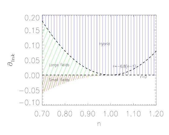
Let us briefly mention where in our parameter space the different inflationary models lie. Traditionally [10] one divides the simplest inflationary models into the following groups: small field $(\alpha<-1)$, large field $(-1<\alpha<1)$, and hybrid models $(\alpha>1)$, where $\alpha$ is defined through the SR parameters (see Appendix A for notation)

$$\eta\equiv\alpha\,\epsilon~{}\,\,\,\,\,{\rm where}\,\,\,\,\,\epsilon=\frac{r}{13.6}\,\,,\,\,\eta=\frac{n-1}{2}+0.15\,r~{}.$$ (4)

Figure 1: The various slow-roll models presented in $(n,\partial_{{\rm ln}k})$ space. The dotted line is the conservative limit, $\epsilon<0.1$. The two dashed lines are the two attractors.

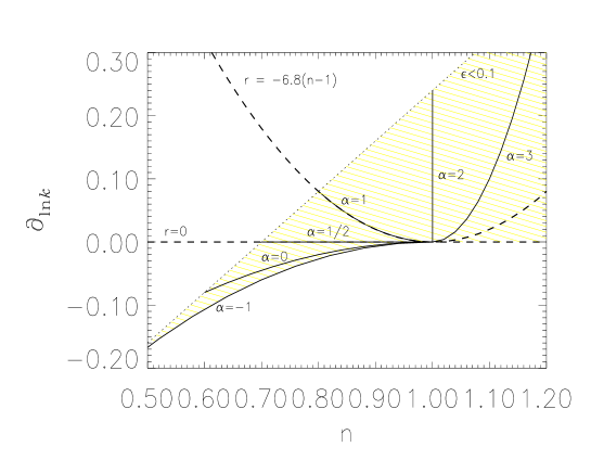
If we for simplicity consider models where the third derivative of the potential is zero ($\xi^{2}=0$), then the different inflationary models are placed in the $(n,\partial_{{\rm ln}k})$-space as shown in Fig. 1, where we have plotted various curves for different $\alpha$. Here we have allowed only the conservative limit $\epsilon<0.1$ (showed by the dotted line), and assumed that we only have to expand the expressions to leading order. Naturally the graph moves up and down by inclusion of the third derivative of the potential, $\xi^{2}\neq 0$. By changing the pivot scale, $k_{0}$, around which the power spectrum is expanded, one can also move the graph sideways (see discussion in section 3), and the $n$ in Fig. 1 should therefore be thought of as the $n$ where the expansion scale has been chosen near the center of the probed scales.

It is interesting that there seems to be attractors in the SR parameter space [11]. The two attractors found in [11] can be expressed as $r=0$ and $r=-6.8(n-1)$, and the behavior of these solutions in the plane $(n,\partial_{{\rm ln}k})$ is shown in Fig. 1 (dashed lines). As one can clearly see, according to these results $\partial_{{\rm ln}k}$ should be positive (or zero). Again, including the third derivative of the potential will also allow for a negative $\partial_{{\rm ln}k}$. From Fig. 2 one sees how these two attractors (dashed lines) are on the borders between the different inflationary models.

Figure 2: The various slow-roll models in $(n,\partial_{{\rm ln}k})$ space. The hybrid models correspond to $\alpha>1$, large fields means $-1<\alpha<1$, and small fields means $\alpha<-1$. The dashed lines are the two attractors.

We will in the present paper discuss the ability of the present day data to provide information on the 3 parameters, $(n,r,\partial_{{\rm ln}k})$.

2 The data

Anisotropies in the CMB were detected for the first time in 1992 by the COBE satellite [12]. Recently, however, our knowledge of the temperature perturbations has increased dramatically with the results from the two balloon-borne experiments Boomerang [13] and MAXIMA [14]. One of the main conclusions from these experiments is the confirmation of the position of the first acoustic peak at $l\sim 200$, which strongly indicates a flat universe, $\Omega_{\rm tot}=1$. This seems to be a confirmation of the inflationary paradigm, since $\Omega_{\rm tot}=1$ is a rather general prediction of the simplest inflationary models. Very interestingly, the data also suggest that the second acoustic peak in the power spectrum is much less pronounced than predicted in flat models with baryon density compatible with BBN [16, 17]. This could be an indication of new physics and accordingly a large number of papers on this subject have appeared since the release of the Boomerang and MAXIMA data. One possibility is that the primordial spectrum of fluctuations produced by inflation is not described by a smooth power-law, but rather that it has bumps and wiggles [18, 19, 20]. In the next section we will discuss this possibility further in light of our numerical results.

The data from Boomerang and MAXIMA was recently analyzed in Ref. [15], where a search in $(n,r)$ space was performed. In that work [15] the assumption was made that $\partial_{{\rm ln}k}=0$, which means that for each set of $(n,r)$ one must carefully adjust the third derivative of the potential to make $\partial_{{\rm ln}k}=0$. This is perfectly possible, but it is more natural to allow $\partial_{{\rm ln}k}$ to vary, as we will do below. The effect of running of the tensor spectral index is very small, but for consistency we include it as described in Eq. (2).

3 Data analysis

In order to to investigate how the new CMB data constrain the parameter space $(n,r,\partial_{{\rm ln}k})$ we have performed a likelihood analysis of the data sets from COBE [12], Boomerang [13] and MAXIMA [14]. The likelihood function to be calculated is

$${\cal L}\propto A\exp\left(-\sum_{i}\frac{(C_{l,i}(\theta)-C_{l,obs,i})^{2}}{\sigma^{2}(C_{l,i})}\right),$$ (5)

where $i$ refers to a specific data point and $\theta$ is a vector of cosmological parameters for the given model

$$\theta=\{\Omega_{m},\Omega_{\Lambda},\Omega_{b},H_{0},\tau,Q,n_{s},r,\partial_{{\rm ln}k},\ldots\}~{}.$$ (6)

In the present case we have calculated the likelihood function for the following parameter space: $\Omega_{m}$, the matter density, $\Omega_{b}$, the baryon density, $H_{0}$, the Hubble parameter, as well as the inflationary parameter space $n,r,\partial_{{\rm ln}k}$. We have assumed that the universe is flat $\Omega_{\Lambda}=1-\Omega_{m}$, and that reionization is not important, $\tau=0$. We also treat the overall normalization, $Q$, as a free parameter. The experimental groups quote estimated calibration errors for the experiments. These should also be accounted for, and we do this by allowing the data points to be shifted up or down by this amount: 10% for Boomerang [13] and 4% for MAXIMA [14]. It should also be noted that the data points are to some extent correllated. The likelihood function, Eq. (5), is based on the assumption that errors are uncorrellated, and therefore a (quite small) error is introduced into our analysis. However, until the full data sets from the experiments are publicly available, the magnitude of the error is difficult to quantify.

Finally, we have chosen the pivot scale in Eq. (1) as $k_{0}=0.05\,{\rm Mpc}^{-1}$. This choice is made for convenience, since $k_{0}=0.05\,{\rm Mpc}^{-1}$ is the scale at which wavenumbers are normalized in the CMBFAST code. Our main results, however, do not depend on the specific value of $k_{0}$.

In Fig. 3 we show the allowed region in the inflationary parameter space for the case corresponding to the calculation of Ref. [15], namely $\partial_{{\rm ln}k}=0$. In the left panel the allowed region was derived assuming that $\Omega_{b}h^{2}=0.019$ (BBN prior [21]), and the left panel of our Fig. 3 thus corresponds to their Fig. 3. Our result is almost identical to theirs, the only difference being that they have used a slightly larger space of other cosmological parameters, so their constraints are slightly less restrictive than ours. In Fig. 4 of Ref. [15], $\tau$ was allowed to vary. Changing the value of $\tau$ does change the likelihood contours (pushing them to larger values of $n$), but only to a small extent. This illustrates that allowing $\tau$ as a free parameter in our analysis would lead to slightly larger allowed regions, but would not in any way invalidate our conclusions.

One thing which should be noticed is that even the best fit point has $\chi^{2}/{\rm d.o.f.}=1.2$, indicating that it is a quite poor fit. This is not too surprising because it is well known that no good fit to the new CMB data can be obtained with a low baryon density, even allowing $r$ to vary [16, 17].

Figure 3: The allowed region in the $n,r$ parameter space, calculated from the combined COBE, Boomerang and MAXIMA data. The dark shaded (green) regions are $1\sigma$ and the light shaded (yellow) are $2\sigma$. The left panel assumes a BBN prior on $\Omega_{b}h^{2}=0.019$, whereas the right panel is for $\Omega_{b}h^{2}=0.030$, the value which best fits the CMB data. Note that the best-fit points, marked by diamonds, are really at $r=0$, but have been shifted slightly so that they are more visible.

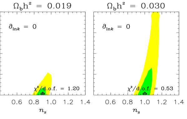
In the right panel we show the allowed region for the case where $\Omega_{b}h^{2}=0.030$, which is the value favored by the CMB measurements. In this case we find an allowed region very similar to that found in Fig. 2 of Ref. [15], although again our allowed region is slightly smaller than theirs because we use a smaller parameter space. It should also be noticed that the best fit point now has $\chi^{2}/{\rm d.o.f.}=0.53$, a very good fit. This corresponds well to the findings of other likelihood analyses [16, 17], that the CMB data can be very well fitted in models with high baryon density.

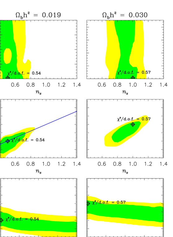
If the assumption $\partial_{{\rm ln}k}=0$ is relaxed, the results change substantially. In Fig. 4 we show results for the likelihood analyses where $\partial_{{\rm ln}k}$ is allowed to vary. Again, the left panels correspond to $\Omega_{b}h^{2}=0.019$ and the right panels to $\Omega_{b}h^{2}=0.030$. As one can see, we have varied the inflationary parameters in a wide range, even larger that what allowed by SR approximation. The reason is that we believe that the main conclusions that we obtain are quite general and give indications on the shape of ${\cal P}(k)$ which are relevant even outside the context of SR models.

In the upper panels of Fig. 4 we show the same allowed region as in Fig. 3, when the assumption $\partial_{{\rm ln}k}=0$ is relaxed. When $\partial_{{\rm ln}k}$ is allowed to vary, the preferred region in parameter space is shifted completely. The best fits are still for a model with no tensor component (for both values of $\Omega_{b}h^{2}$), but now there is no real constraint on $r$. The best fit models now have $\chi^{2}/{\rm d.o.f.}=0.54$ and 0.57 respectively, which indicate very good fits.

Figure 4: The allowed region in the $n,r,\partial_{{\rm ln}k}$ parameter space, calculated from the combined COBE, Boomerang and MAXIMA data. The dark shaded (green) regions are $1\sigma$ and the light shaded (yellow) are $2\sigma$. The left panels assume a BBN prior on $\Omega_{b}h^{2}=0.019$, whereas the right panels are for $\Omega_{b}h^{2}=0.030$, the value which best fits the CMB data. Note that the best-fit points, marked by diamonds, are really at $r=0$, but have been shifted slightly so that they are more visible. The solid line in the left $(n,\partial_{{\rm ln}k})$ panel corresponds to the power spectrum exhibiting a distinct feature at $k=0.004\,{\rm Mpc}^{-1}$ (see Eq. (8) and the surrounding discussion).

Figure 5: Power spectra for four different models. Panel (a) is the best fit model with $\partial_{{\rm ln}k}=0,r=0$, (b) the best fit with $\partial_{{\rm ln}k}=0,r=2$, (c) the best fit with $\partial_{{\rm ln}k}\neq 0,r=0$, and (d) the best fit with $\partial_{{\rm ln}k}\neq 0,r=2$. The data points are from the Boomerang experiment [13]. The curves show: The scalar component (dotted lines), tensor component (dashed lines), and the combined fluctuation spectrum (solid lines).

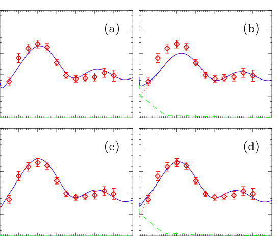
In order to understand why allowing $\partial_{{\rm ln}k}$ to vary erases any ability to constrain $r$, it is instructive to look at the power spectra for some of the best fit models directly. For the remainder of this section we will assume that $\Omega_{b}h^{2}=0.019$, in accordance with Big Bang nucleosynthesis. In Fig. 5 we show four different power spectra, all calculated for the case of $\Omega_{b}h^{2}=0.019$. Panels (a) and (b) are both for $\partial_{{\rm ln}k}=0$. Model (a) is the best fit with $r=0$, whereas (b) is the best fit with $r=2$. Model (b) is a very poor fit because introducing a tensor component while still fitting the high $l$-values severely underestimates power around the first peak. This cannot be remedied by shifting $n$ alone. Therefore, the allowed values of $r$ are quite tightly constrained.

Panels (c) and (d), on the other hand, show models where $\partial_{{\rm ln}k}$ is allowed to vary. Model (c) is the best fit for $r=0$ and (d) is the best fit for $r=2$. In contrast to the case with $\partial_{{\rm ln}k}=0$, it is possible to obtain a decent fit, even with a large tensor component because the power spectrum can be “bent” by having a non-zero $\partial_{{\rm ln}k}$.

Figure 6: Power spectra of scalar perturbations for selected values of the parameters $(n,\partial_{{\rm ln}k})$ which provide good fits to the CMB data. The solid line corresponds to the best-fit point, $(n,\partial_{{\rm ln}k})=(0.5,-0.2)$. The dashed lines correspond, from top to bottom in the maximum region, to $(n,\partial_{{\rm ln}k})$ equal to $(0.4,-0.24)$, $(0.6,-0.16)$, $(0.7,-0.12)$, respectively. The dot-dashed line corresponds to best-fit model with constant spectral index, i.e. $(n,\partial_{{\rm ln}k})=(0.9,0)$. All normalizations are arbitrary.

The effect of a running spectral index can also be understood by looking at Fig. 6, where we show the power spectra of scalar perturbations corresponding to values of $(n,\partial_{{\rm ln}k})$ which provide good fits to the CMB data. The effects of a $\partial_{{\rm ln}k}\neq 0$ is somewhat similar to introduce a feature in the power spectrum at a fixed scale. Specifically, for $\partial_{{\rm ln}k}<0$, the power spectra show a maximum at a scale $k_{m}$ given by

$$\ln(k_{m}/k_{0})=-(n-1)/\partial_{{\rm ln}k}.$$ (7)

The CMB data provide a constraint for the possible positions of this maximum. This can be understood by looking at the left $(n,\partial_{{\rm ln}k})$ panel of Fig. 4, from which it is evident that the allowed region in the plane $(n,\partial_{{\rm ln}k})$ lies along a line corresponding to $k_{m}=const$. Specifically, the best fit model corresponds to $k_{m}=0.004\,\rm{Mpc}^{-1}$, while possible values are $k_{m}=0.0015-0.01\,\rm{Mpc}^{-1}$.

It is easy to understand why such a feature helps to fit the CMB data. In order to increase sizeably the first to second peak ratio in the CMB, one needs a power spectrum with a large negative slope at intermediate and small scales, say e.g. $k>0.01\;\rm{Mpc}^{-1}$. If we assume $\partial_{{\rm ln}k}=0$ this is not allowed; the power spectrum is then a monotonic function of $k$ and, as consequence, one automatically obtains an excess of power at large scales, corresponding to COBE normalization. If instead one has $\partial_{{\rm ln}k}\leq 0$, the power spectrum is non-monotonic and has a maximum at a specific scale $k_{m}$. Specifically, if $k_{m}\simeq 0.004\;\rm{Mpc}^{-1}$, the power spectrum decreases both at large and at small scales so that one has no trouble in reproducing the COBE data. Clearly, as a by-product, one looses the ability to constrain the tensor to scalar ratio $r$. The scalar power spectrum at large scale can in fact be strongly suppressed and this allows for a large contribution from tensor perturbations.

We conclude this section by comparing our result with the result of [18], in which a Gaussian bump in $\log k$ was added to a standard power spectrum and its position $k_{b}$ was constrained by CMB data. In very nice agreement with our results they found a best fit $k_{b}$ of roughly $0.005h\;\rm{Mpc}^{-1}$, and an allowed region for $k_{b}$ of $0.001h-0.01h\;\rm{Mpc}^{-1}$.

4 Conclusion

We have considered the ability of the present day CMBR data to distinguish between various slow-roll models of inflation, allowing the scalar spectral index, $n(k)$, to vary with scale. Specifically, we have expanded the power spectrum ${\cal P}(k)$ to second order in $\ln k$ and we have derived the constraints on the parameter space $(n,r,\partial_{{\rm ln}k})$ which can be obtained by using COBE, Boomerang and MAXIMA data.

We have seen that:

i) If we allow $\partial_{{\rm ln}k}\neq 0$ the tensor to scalar ratio $r$ is essentially unconstrained, even if we assume $\Omega_{b}h^{2}$ as low as suggested by BBN considerations.

Moreover, assuming a BBN prior of $\Omega_{b}h^{2}=0.019$, we have found that:

ii) A negative bend of the power spectrum, $\partial_{{\rm ln}k}\leq 0$, is favoured by the CMB data.

iii) The best fit model, $(n,\partial_{{\rm ln}k})=(0.5,-0.2)$, which provides a very good fit to the CMB, corresponds to a power spectrum which deviates quite strongly from a power law approximation. The large values obtained for $n-1$ and $\partial_{{\rm ln}k}$ are bordering to invalidate the slow-roll approximation, however, one should keep in mind that changing the pivot scale, $k_{0}$, will change the value of $n-1$, and inclusion of the 3^rd derivative of the inflaton potential will change the value of $\partial_{{\rm ln}k}$;

iv) The CMB data favor power spectra with a bump-like feature at scales $k_{m}=0.0015-0.01\,{\rm Mpc}^{-1}$, the best fit value being $k_{m}=0.004\,{\rm Mpc}^{-1}$.

Summarizing, the general result of our analysis is that a single power law for ${\cal P}(k)$ does not provide a good fit to CMB data, if we assume a BBN prior $\Omega_{b}h^{2}=0.019$. In particular, CMB data favor models in which ${\cal P}(k)$ deviates strongly from a power law approximation. Specifically, the scale at which the power law approximation should be broken, i.e. second (or higher) order terms in eq. (1) become important, is $k=0.0015-0.01\,\rm{Mpc}^{-1}$.

Appendix A Notation

We use the notation:

$$\epsilon=\frac{M^{2}}{2}\left(\frac{V^{\prime}}{V}\right)^{2}\,\,\,\mbox{and}\,\,\,\eta=M^{2}\frac{V^{\prime\prime}}{V}-\frac{M^{2}}{2}\left(\frac{V^{\prime}}{V}\right)^{2}~{},$$

see [15] for details. The notation with $\eta=M^{2}V^{\prime\prime}/V$, used e.g. in [2], simply corresponds to the substitution $\alpha\rightarrow\alpha+1$ in eq.(4). Independently on the chosen definition for $\eta$, one finds

$$\partial_{{\rm ln}k}=-2\xi^{2}+4\,\frac{r}{6.8}\left[(n-1)+\frac{3}{2}\frac{r}{6.8}\right]~{},$$ (8)

where $\xi^{2}\equiv M^{4}V^{\prime}V^{\prime\prime\prime}/V^{2}$. One could potentially include higher order terms in Eq. (1), corresponding to $d^{2}n/d{\rm ln}k^{2}\neq 0$, which would be expressed as

$$\frac{d^{2}n_{S}}{d{\rm ln}k^{2}} = 2\sigma^{3}+\frac{1}{2}\partial_{{\rm ln}k}\left(9\frac{r}{6.8}-(n-1)\right)$$ (10)

$$-2\left(n-1\right)^{2}\frac{r}{6.8}-15\left(n-1\right)\left(\frac{r}{6.8}\right)^{2}-15\left(\frac{r}{6.8}\right)^{3}~{},$$

$$\frac{d^{2}n_{T}}{d{\rm ln}k^{2}} = \partial_{{\rm ln}k}\frac{r}{6.8}-\left(n-1\right)^{2}\frac{r}{6.8}-3\left(n-1\right)\left(\frac{r}{6.8}\right)^{2}-2\left(\frac{r}{6.8}\right)^{3}~{},$$ (11)

with $\sigma^{3}\equiv 2\epsilon V^{\prime\prime\prime\prime}/V$.

References

- [1] J. E. Lidsey, A. R. Liddle, E. W. Kolb, E. J. Copeland, T. Barreiro and M. Abney, Rev. Mod. Phys. 69 (1997) 373.
- [2] D. H. Lyth and A. Riotto, Phys. Rept. 314 (1999) 1.
- [3] A. R. Liddle and D. H. Lyth, Phys. Lett. B291 (1992) 391.
- [4] A. Kosowsky and M. S. Turner, Phys. Rev. D52 (1995) 1739.
- [5] L. Knox, Phys. Rev. D52 (1995) 4307 M. S. Turner and M. White, Phys. Rev. D53 (1996) 6822.
- [6] E. D. Stewart, Phys. Lett. B391 (1997) 34; Phys. Rev. D56 (1997) 2019.
- [7] W. H. Kinney and A. Riotto, Phys. Lett. B435 (1998) 272.
- [8] E. J. Copeland, I. J. Grivell and A. R. Liddle, astro-ph/9712028.
- [9] L. Covi and D. H. Lyth, Phys. Rev. D59 (1999) 063515.
- [10] S. Dodelson, W. H. Kinney and E. W. Kolb, Phys. Rev. D56 (1997) 3207.
- [11] M.B. Hoffman & M.S. Turner, astro-ph/0006321.
- [12] G. F. Smoot et al., Astrophys. J. Lett. 396, L1 (1992).
- [13] P. de Bernardis et al., Nature 404 (2000) 955; A.E. Lange et al., astro-ph/0005004.
- [14] S. Hanany et al., astro-ph/0005123; A. Balbi et al., astro-ph/0005124.
- [15] W. H. Kinney, A. Melchiorri and A. Riotto, astro-ph/0007375.
- [16] A. H. Jaffe et al., astro-ph/0007333.
- [17] M. Tegmark, M. Zaldarriaga and A. J. S. Hamilton, astro-ph/0008167.
- [18] L. Griffiths, J. Silk and S. Zaroubi, astro-ph/0010571.
- [19] J. Barriga et al., astro-ph/0011398.
- [20] Y. Wang and G. Mathews, astro-ph/0011351.
- [21] S. Burles, K. M. Nollett and M. S. Turner, astro-ph/0008495.