The solar dynamo: old, recent, and new problems

Abstract

A number of problems of solar and stellar dynamo theory are briefly reviewed and the current status of possible solutions is discussed. Results of direct numerical simulations are described in view of mean-field dynamo theory and the relation between the $\alpha$-effect and the inverse cascade of magnetic helicity is highlighted. The possibility of ‘catastrophic’ quenching of the $\alpha$-effect is explained in terms of the constraint placed by the conservation of magnetic helicity.

NORDITA, Blegdamsvej 17, DK-2100 Copenhagen Ø, Denmark; and
Department of Mathematics, University of Newcastle upon Tyne, NE1 7RU, UK

1. Introduction

The solar dynamo problem has always been plagued by a number of problems. One of the most outstanding is the question of why the solar dynamo wave travels toward the equator and not the other way around. According to $\alpha\Omega$-dynamo theory the dynamo wave travels equatorward only if the sign of the product of alpha-effect and radial angular velocity gradient, $\partial\Omega/\partial r$, is negative. However, cyclonic convection gives rise to a positive $\alpha$-effect (Parker 1955, Steenbeck, Krause, & Rädler 1966), so one needs a negative sign of $\partial\Omega/\partial r$. Thus, a problem has arisen since the mid-eighties (Parker 1987), i.e. since helioseismology took away the freedom of dynamo theorists to adopt a suitable rotation profile. This left only the choice of adopting an appropriate profile (and sign!) for the alpha-effect. Not surprisingly, dynamo theorists were labelled as being able to reproduce almost anything, but in reality they were not even able to do that, because there was one more problem: the phase relation between poloidal and toroidal fields (Stix 1976). The sign of the mean radial magnetic field, ${\overline{B}}_{r}$, is observed to be almost always opposite to the sign of the mean toroidal field, ${\overline{B}}_{\phi}$. The phase relation between ${\overline{B}}_{r}$ and ${\overline{B}}_{\phi}$ is determined directly by $\partial\Omega/\partial r$, because the shear turns radial field into toroidal. This problem is actually rather general in its nature and quite independent of dynamo theory.

One possible solution to this dynamo dilemma (Parker 1987) may lie in the possibility that the sense of the dynamo wave can be determined by the sense of the meridional circulation: a poleward circulation in the upper layers corresponds to equatorward motion in the lower layers, and if the sunspot activity is governed by fields at the bottom of the convection zone this circulation may control the migration of activity regions Durney 1996, Choudhuri et al. 1996). A systematic survey of solutions with meridional circulation (Küker et al. 2000) has revealed that the sense of the dynamo wave is reversed only if the following conditions are met: the magnetic eddy diffusivity is small enough, the circulation is strong enough, and the $\alpha$-effect is sufficiently supercritical. If this is the case, Küker et al. (2000) also find ${\overline{B}}_{r}$ and ${\overline{B}}_{\phi}$ to be approximately in antiphase, as observed.

Over the past ten years some rather more fundamental problems have shadowed the attempts to model closely the solar field geometry: does the $\alpha$-effect really work in high Reynolds number flows like the sun, or is it totally suppressed by the magnetic field?

2. The helicity constraint

A serious problem that has only recently received attention results from magnetic helicity conservation. The problem is relatively easily explained and applies to all fields that have magnetic helicity. In particular, it applies to the large scale magnetic fields generated by $\alpha^{2}$ or $\alpha\Omega$ dynamos, but not, for example, to fields generated by a small scale dynamo which may produce significant helicity fluctuations, but no net magnetic helicity.

Magnetic helicity can only change resistively or through flux on the boundaries. Thus, a large scale field with magnetic helicity can only be generated on a resistive timescale or, if there are suitable losses of the right kind on the boundaries, field generation can proceed on a dynamical timescale. The latter alternative is not straightforward, because such losses always involve losses of magnetic energy too. This latter alternative will be discussed later. First, however, we shall look more quantitatively at the consequences of resistively slow changes of helicity in closed or periodic boxes.

The condition of helicity conservation together with the assumption that the large scale field is helical result in a simple condition for the energy of the mean magnetic field (Brandenburg 2000, hereafter referred to as B2000)

$$\langle\overline{\mbox{\boldmath$B$}}^{2}\rangle/B_{\rm eq}^{2}\approx k_{\rm f}\ell_{AB}\left[1-\exp(-2\eta k_{1}^{2}(t-t_{\rm sat})\right],$$ (1)

where $k_{\rm f}$ is the wavenumber of the (kinetic) energy carrying eddies (e.g. the forcing wavenumber), $k_{1}$ is the smallest possible wavenumber, $\eta$ is the microscopic magnetic diffusivity, $t$ is time, $t_{\rm sat}$ is the time when the field at small and intermediate scales saturates, and $\ell_{AB}$ quantifies the degree to with the large scale field is helical. This relation is rather general and independent of the actual model of field amplification. If the field is not fully helical, then $\ell_{AB}$ will be reduced, but the important point here is that full saturation is only obtained after a large scale ohmic diffusion time, $1/\eta k_{1}^{2}$.

The important point is that all box simulations with helicity have to obey this behavior. This is shown in Fig. 1 for one particular example, but this constraint is indeed very well obeyed by all other simulations presented in B2000.

Figure 1.: Evolution of $\langle\overline{\mbox{\boldmath$B$}}^{2}\rangle$ for Run 3 of B2000, compared with the constraint imposed by helicity conservation (dashed lines). Also plotted is the result of a mean-field dynamo with ‘catastrophic’ alpha and eta quenching (dotted lines).

The helicity constraint has two properties: full saturation of the large scale field (as opposed to the small scale field) happens on a resistive time scale, $1/\eta k_{1}^{2}$, and secondly, the energy of the maximum field strength in units of the equipartition field strength is given by the product $k_{\rm f}\ell_{AB}$, and for maximally helical fields we have $\ell_{AB}=k_{1}^{-1}$. In our particular runs we have $k_{\rm f}/k_{1}=5$, so we can reach maximally five times supercritical energies of the large scale field. (In B2000 there is also run with $k_{\rm f}/k_{1}=30$, which does indeed give correspondingly higher field strengths.) The reason we have this factor 5 here can be motivated as follows. The large scale dynamo is driven by some effective $\alpha$ which has contributions from the kinetic helicity and the current helicity of the small scale field which combine to a residual helicity (Pouquet et al. 1976, Field et al. 1999). Near equipartition the residual helicity is very small, so kinetic helicity and small scale current helicity nearly balance each other. The kinetic helicity, $\langle\mbox{\boldmath$\omega$}{}\cdot\mbox{\boldmath$u$}{}\rangle$, is proportional to $k_{\rm f}\langle\mbox{\boldmath$u$}{}^{2}\rangle$, so we know how big that is. On the other hand, the small scale current helicity, $\langle\mbox{\boldmath$j$}{}\cdot\mbox{\boldmath$b$}{}\rangle$, is exactly the term which drives magnetic helicity, $\langle\mbox{\boldmath$A$}{}\cdot\mbox{\boldmath$B$}{}\rangle$. In the steady state $\langle\mbox{\boldmath$A$}{}\cdot\mbox{\boldmath$B$}{}\rangle$ can no longer change, so $\langle\mbox{\boldmath$j$}{}\cdot\mbox{\boldmath$b$}{}\rangle$ must be balanced with the contribution from large scales, $\langle\overline{\mbox{\boldmath$J$}}\cdot\overline{\mbox{\boldmath$B$}}\rangle$, which determine then the large scale field strength, $\langle\overline{\mbox{\boldmath$J$}}\cdot\overline{\mbox{\boldmath$B$}}\rangle=k_{1}\langle\overline{\mbox{\boldmath$B$}}^{2}\rangle$. This is – in words – the reason why superequipartition field strengths can be attained. (For mathematical details see B2000.)

2.1. Catastrophic quenching

Exactly the same resistive behavior as in Eq. (1) can be reproduced using the $\alpha^{2}$ dynamo equation (e.g. Moffatt 1978) with simultaneous quenching of $\alpha$ and the turbulent magnetic diffusivity, $\eta_{\rm t}$, in the form

$$\alpha={\alpha_{0}\over 1+\alpha_{B}\overline{\mbox{\boldmath$B$}}^{2}\!/B_{\rm eq}^{2}},\quad\eta_{\rm t}={\eta_{\rm t0}\over 1+\eta_{B}\overline{\mbox{\boldmath$B$}}^{2}\!/B_{\rm eq}^{2}},$$ (2)

where we assume $\alpha_{B}=\eta_{B}$. We focus here on the case of homogeneous turbulence in which case the large scale magnetic field is a force-free field whose energy density is very nearly uniform, so $\overline{\mbox{\boldmath$B$}}^{2}$ is just a function of time and we can obtain the solution $\overline{\mbox{\boldmath$B$}}=\overline{\mbox{\boldmath$B$}}(t)$ in closed form (B2000).

A natural by-product of this model is that the quenching coefficient $\alpha_{B}$ (which is assumed to be the same as $\eta_{B}$) must be proportional to the magnetic Reynolds number! This type of quenching was suggested earlier on phenomenological grounds by Cattaneo & Vainshtein (1991) and Vainshtein & Cattaneo (1992), but the conclusion was thought to be that for dynamically important field strengths ($|\overline{\mbox{\boldmath$B$}}|\rightarrow B_{\rm eq}$) the two turbulent transport coefficients would be so strongly quenched that such fields cannot be the result of a mean-field dynamo. That was the reason that such quenching was referred to as ‘catastrophic’. We now see however that there is nothing catastrophic about it and that field strength even in excess of $B_{\rm eq}$ can be generated.

The significance of these results is that they provide an excellent fit to the numerical simulations; see Fig. 1 where we present the evolution of $\langle\overline{\mbox{\boldmath$B$}}^{2}\rangle$ for Run 3 of B2000. The dynamo equations with appropriate quenching expressions can therefore be used to extrapolate to astrophysical conditions. The time $\tau_{\rm eq}$ required to convert the small scale field generated by the small scale dynamo to a large scale field increases linear with the magnetic Reynolds number, $R_{\rm m}$. Apart from some coefficients of order unity the ratio of $\tau_{\rm eq}$ to the turnover time is therefore just $R_{\rm m}$. For the sun this ratio would be $10^{8}-10^{10}$. However, before interpreting this result further one really has to know whether or not the presence of open boundary conditions could alleviate the issue of very long timescales for the mean magnetic field. Furthermore, it is not clear whether the long timescales discussed above have any bearing on the cycle period in the case of oscillatory solutions. The reason this is not so clear is because for a cyclic dynamo the magnetic helicity in each hemisphere stays always of the same sign and is only slightly modulated. It is likely that this modulation pattern is advected precisely with the meridional circulation, in which case the helicity could be nearly perfectly conserved in a lagrangian frame. This would support the suggestion of Durney (1995) and Choudhuri, Schüssler, & Dikpati (1995) that the dynamo wave travels mainly because of meridional circulation.

3. Quadratic or cubic quenching?

When the first nonlinear mean-field dynamo models with $\alpha$-quenching were calculated numerically (e.g., Jepps 1975, Ivanova & Ruzmaikin 1977), a simple quenching formula of the form $\alpha\sim 1/(1+B^{2})$ was used. This was really nothing more than just a simple fix to the problem that a quadratic formula of the form $\alpha\sim 1-B^{2}$ may overshoot and change sign. We emphasize that a quenching formula of the form $\alpha\sim 1/(1+B^{2})$ was never obtained rigorously. Instead, the correct quenching behavior, at least in the low magnetic Reynolds number limit, had cubic limiting behavior (Moffatt 1972, Rüdiger 1974).

We are now for the first time in a position to check whether the limiting behavior for higher magnetic Reynolds numbers is quadratic or cubic. In Fig. 2 we plot the evolution of the magnetic energy for a model with cubic $\alpha$-quenching,

$$\alpha=\alpha_{0}/[1+(\alpha_{B}\overline{\mbox{\boldmath$B$}}^{2}/B_{\rm eq}^{2})^{n}],\quad n=3/2.$$ (3)

It turns out that in this case the evolution of $\overline{\mbox{\boldmath$B$}}^{2}$ does not agree with the limiting behavior enforced by the helicity constraint (1); see Fig. 2. This confirms that the phenomenological expression (2) is actually correct, at least for the homogeneous $\alpha^{2}$ dynamo. (We shall see later that for inhomogeneous dynamos with shear the tensorial nature of $\alpha$-effect and turbulent diffusivity cannot be ignored, and that the quenching works differently for different components.)

Figure 2.: Clear disagreement between mean-field model with cubic quenching formula (solid line) and the result from the helicity constraint (dashed line). For comparison the helicity constraint formula with a $3\eta$ factor (instead of $2\eta$) is also shown as open symbols.

One might think that a catastrophic quenching expression of the form $1-\alpha_{B}\overline{\mbox{\boldmath$B$}}^{2}\!/B_{\rm eq}^{2}$, as opposed to $1/(1+\alpha_{B}\overline{\mbox{\boldmath$B$}}^{2}\!/B_{\rm eq}^{2})$, for both $\alpha$ and $\eta_{\rm t0}$ may also reproduce the resistively dominated growth of the field, but this is not the case. To show this we consider the steady state of the $\alpha^{2}$-dynamo in the one-mode approximation, so

$${{\rm d}{}\ln\overline{\mbox{\boldmath$B$}}^{2}\over{\rm d}{}t}=0=(\alpha_{0}k-\eta_{\rm t0}k^{2})(1-\alpha_{B}\overline{\mbox{\boldmath$B$}}^{2}\!/B_{\rm eq}^{2})-\eta k^{2},$$ (4)

which leads to the final field strength $B_{\rm fin}$ given by

$$\alpha_{B}B_{\rm fin}^{2}/B_{\rm eq}^{2}=1-{\eta k^{2}\over\alpha_{0}k-\eta_{\rm t0}k^{2}}={\alpha_{0}k-\eta_{\rm T0}k^{2}\over\alpha_{0}k-\eta_{\rm t0}k^{2}}\approx 1,$$ (5)

where $\eta_{\rm T0}=\eta+\eta_{\rm t0}$ is the total (microscopic plus turbulent) magnetic diffusivity. Since we know from the simulations that $B_{\rm fin}/B_{\rm eq}={\cal O}(1)$, Eq. (5) implies that $\alpha_{B}={\cal O}(1)$, which would then not reproduce the resistively dominated growth.

In order to appreciate the difference to a quenching formula of the form $1/(1+\alpha_{B}\overline{\mbox{\boldmath$B$}}^{2}\!/B_{\rm eq}^{2})$, we write down the corresponding equation for that case:

$${{\rm d}{}\ln\overline{\mbox{\boldmath$B$}}^{2}\over{\rm d}{}t}=0={\alpha_{0}k-\eta_{\rm t0}k^{2}\over 1+\alpha_{B}\overline{\mbox{\boldmath$B$}}^{2}\!/B_{\rm eq}^{2}}-\eta k^{2},$$ (6)

so

$$0=\alpha_{0}k-\eta_{\rm t0}k^{2}-\eta k^{2}(1+\alpha_{B}\overline{\mbox{\boldmath$B$}}^{2}\!/B_{\rm eq}^{2})=\alpha_{0}k-\eta_{\rm T0}k^{2}-\eta k^{2}\alpha_{B}\overline{\mbox{\boldmath$B$}}^{2}\!/B_{\rm eq}^{2},$$ (7)

which leads to a final field strength $B_{\rm fin}$ given by

$$\alpha_{B}B_{\rm fin}^{2}/B_{\rm eq}^{2}={\alpha_{0}k-\eta_{\rm T0}k^{2}\over\eta k^{2}}\gg 1,$$ (8)

so $B_{\rm fin}/B_{\rm eq}={\cal O}(1)$ implies $\alpha_{B}\gg 1$, as in Eq. (2), which we know leads to resistively dominated growth.

Although we cannot exclude that there may be other possible quenching formulae than Eq. (2), it is clear that it is easy to come up with other plausible choices which do not obey the helicity constraint (1). However, despite its success, (1) cannot be regarded as fundamental in that under other circumstances it may not describe the $\alpha$-effect correctly. In the following we describe first an example where Eq. (2) gives a good prediction of what is then also verified in simulations, and then we turn to another example where Eq. (2) does poorly.

4. Open boundaries

The main problem of why the saturation of the large scale dynamo progresses on a resistive timescale is, mathematically speaking, that there is no other term on the right hand side of the magnetic helicity equation. However, this changes if the volume under consideration is no longer periodic or closed, so that there can be a transport of magnetic helicity through the boundaries. However, what tends to happen is that the loss of helicity occurs mostly on large scales. Associated with this is a significant loss of large scale magnetic energy. Thus, although it is true that the time scale gets reduced, the saturation energy decreases, making it harder to reach significant field strengths of the large scale field. (The small scale field is unaffected by this.) In fact, looking at the field evolution on an absolute scale shows that the loss of magnetic helicity and energy simply terminates the growth at a lower level; see Fig. 3.

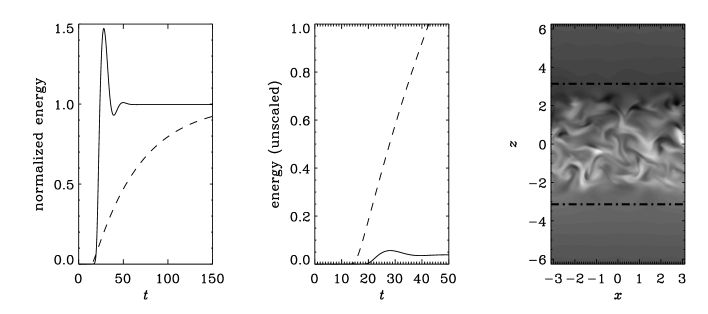
Figure 3.: Evolution of magnetic energy (first panel: normalized to the final value, second panel: unscaled) for a mean-field model with catastrophic quenching and either open boundaries (solid lines) or periodic boundaries (dashed lines). In the third panel we show a meridional cross-section of the toroidal magnetic field from a simulation with open boundaries in the $z$-direction at $\pm\pi$. Different shades represent different values of the toroidal field strength. The parameters of the mean-field model are $\alpha_{0}=2$, $\eta_{\rm t0}=1$, $\eta=0.01$, $k=1$, so the kinematic growth rate is $\lambda=\alpha_{0}k-\eta_{\rm t0}k^{2}=1$, and with $k_{\rm f}=5$ we have $\alpha_{B}=\lambda/(\eta kk_{\rm f})=20$. In the non-periodic case a vertical field boundary condition was adopted.

One may speculate that lower saturation levels are still acceptable in many astrophysical settings, because if the dynamo is sufficiently supercritical (like in accretion discs and many stars, but possibly not in galaxies), the tendency to reduce the saturation level could be offset by a correspondingly stronger dynamo.

5. The effects of shear

The presence of shear is interesting because in that case oscillatory solutions can be expected. This is indeed what happens; see the butterfly diagram in Fig. 4. In this model the oscillation frequency is $2\pi/1000\approx 0.006$ (in nondimensional units). This value lies just between the ohmic and dynamic rates of change, $\eta k_{1}^{2}=5\times 10^{-4}$ and 0.08, respectively. This suggests that the cycle period is not affected by the magnetic helicity constraint in the same way as the growth time of the dynamo, which is a resistive timescale. For a full account of this work see Brandenburg et al. (2000).

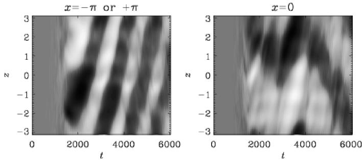
Figure 4.: Butterfly (space-time) diagram of the toroidal mean field at two different $x$-positions where the sign of the shear is either negative or positive, giving rise to dynamo waves traveling in opposite direction.

6. Conclusions

An important step has been reached in modelling dynamo action in astrophysics in that we are now beginning to bridge the gap between direct three-dimensional simulations on the one hand and the mean-field approach on the other. Many of the conclusions reached earlier in the framework of mean-field theory do apply, but there are also important restrictions. Most importantly, the alpha and eta coefficients have to obey some rather general restrictions resulting from helicity conservation. Further extensions to the theory, for example the inclusion of open boundaries, can straightforwardly be modelled. However, it seems that open boundaries do not enhance dynamo action, as one may have hoped, but instead they lead to a lower field strength at saturation, which is now however reached earlier on a dynamical timescale. In the presence of shear the helicity constraint still applies, but the modelling in terms of mean-field theory is not yet fully understood because anisotropies in the quenching become very important.

References

Brandenburg, A. 2000, ApJ (submitted) astro-ph/0006186 (B2000).

Brandenburg, A., Bigazzi, A., & Subramanian, K. 2000, MNRAS, astro-ph/0011081

Cattaneo, F., & Vainshtein, S. I. 1991, ApJ (Letters) 376, L21

Choudhuri, A. R., Schüssler, M., & Dikpati, M. 1995, A&A 303, L29

Durney, B. R. 1995, Solar Phys. 166, 231

Ivanova, T. S., & Ruzmaikin, A. A. 1977, Sov. Astron. 21, 479

Field, G. B., Blackman, E. G., & Chou, H. 1999, ApJ 513, 638

Jepps, S. A. 1975, JFM 67, 625

Küker, M., Rüdiger, G., & Schultz, M. 2000, A&A (submitted)

Moffatt, H. K. 1972, JFM 53, 385

Moffatt, H. K. 1978, Magnetic Field Generation in Electrically Conducting Fluids (Cambridge University Press, Cambridge)

Parker, E. N. 1955, ApJ 121, 491

Parker, E. N. 1987, Solar Phys. 110, 11

Pouquet, A., Frisch, U., & Léorat, J. 1976, JFM 77, 321

Rüdiger, G. 1974, Astr. Nachr. 295, 275

Steenbeck, M., Krause, F., & Rädler, K.-H. 1966, Z. Naturforsch. 21a, 369

Stix, M. 1976, A&A 47, 243

Vainshtein, S. I., & Cattaneo, F. 1992, ApJ 393, 165