AD Leo from X-Rays to Radio: Are Flares Responsible for the Heating of Stellar Coronae?

Abstract

In spring 1999, a long coordinated observing campaign was performed on the flare star AD Leo, including EUVE, BeppoSAX, the VLA, and optical telescopes. The campaign covered a total of 44 days. We obtained high-quality light curves displaying ongoing variability on various timescales, raising interesting questions on the role of flare-like events for coronal heating. We performed Kolmogorov-Smirnov tests to compare the observations with a large set of simulated light curves composed of statistical flares that are distributed in energy as a power law of the form ${\rm d}N/{\rm d}E\propto E^{-\alpha}$ with selectable index $\alpha$. We find best-fit $\alpha$ values slightly above a value of 2, indicating that the extension of the flare population toward small energies could be important for the generation of the overall X-ray emission.

Paul Scherrer Institut, Würenlingen and Villigen, CH-5232 Villigen PSI, Switzerland

Dept. of Astronomy & Astrophysics, Villanova University, Villanova, PA 19085, USA

Harvard-Smithsonian Center for Astrophysics, Cambridge, MA 02138, USA

SRON, Sorbonnelaan 2, 3584 CA Utrecht, The Netherlands

Crimean Astrophysical Observatory, Nauchny, Crimea 334413, Ukraine

1. Introduction

While large, episodic stellar flares heat coronal plasma rather efficiently up to 100 MK for minutes to hours, it is the potentially large number of small, and even ‘undetected’ flares (“microflares”, “nanoflares”, e.g., Parker 1988) that have recently attracted the attention of both solar and stellar research. Solar observations show that the flare occurrence rate is distributed in energy as a power law,

$${{\rm d}N\over{\rm d}E}\propto E^{-\alpha}$$ (1)

(e.g., Lin et al. 1984). The value of $\alpha$ determines the importance of the low- or high-energetic tail of the distribution: The integration of the energy over the energy distribution (1)

$$L_{\rm X}\propto\int_{\rm E_{\rm min}}^{\rm E_{\rm max}}{{\rm d}N\over{\rm d}E}E{\rm d}E$$ (2)

with $\alpha\geq 2$ produces arbitrarily large total emission rates if $E_{\rm min}\rightarrow 0$ (microflares, nanoflares). There is ample evidence that the ensemble of flares play a fundamental role in the heating of (quiescent) coronae of magnetically active stars:

• Active stars emit strong gyrosynchrotron radio emission during quiescence: Evidence for accelerated (MeV) electrons as in solar flares (Güdel 1994).

• This non-thermal emission correlates with the overall X-ray radiation the same way as solar flares do (Güdel & Benz 1993; Benz & Güdel 1994).

• The optical U band flare frequency correlates with the quiescent X-ray stellar luminosity (Doyle & Butler 1985).

• Transition region lines show broadening probably related to explosive events (Wood et al. 1996).

• Small flare events with energies of the order of $10^{27}-10^{28}$ ergs have become observable with the Hubble Space Telescope in cool M dwarfs, proving their ubiquity in active stellar atmospheres (Robinson et al. 1995).

• The structuring of X-ray emitting active coronae is reminiscent of the thermal structure of flares (Güdel et al. 1997) and may be explained by the superposition of a distribution of statistical flares (Kopp & Poletto 1993; Güdel 1997).

• Solar observations now show the importance of micro- and nanoflares in coronal energy release: $\alpha=2.3-2.6$ for microflares in the quiet corona (Krucker & Benz 1998).

Studies of statistical flare distributions have been rare in the stellar context, due to the paucity of relevant data sets. Collura et al. (1988) found a power-law index $\alpha=1.52$ from EXOSAT observations of dMe stars, while Osten & Brown (1999) report $\alpha=1.6$ for a sample of RS CVn binary systems observed with EUVE. In a series of papers (Audard, Güdel, & Guinan 1999; Audard et al. 2000; Güdel et al. 2000a) we have been investigating systematically the role of statistical flares in the overall coronal heating of active stars. From a large sample of EUVE observations, we found that

• relatively steep ($\alpha=2-2.5$) power laws dominate the flare rate distributions, indicating that small flares are important in these coronae.

• Statistical heating by flares leads to dominant coronal temperatures in agreement with the measurements.

2. New Observations of AD Leo: Flares over and over again

An extremely long EUVE observation of AD Leo was approved during EUVE’s cycle 7 between April 2 and May 16, 1999 (with a few minor time gaps) comprising 900 ksec of on-source exposure time. The DS instrument and the three spectrometers (SW, MW, LW) were used. Between May 1 and May 15, we obtained a total of 270 ks of exposure time with BeppoSAX, covering about 8 days within this interval. We obtained data from the LECS (0.1–10 keV), the MECS (2–10 keV), and the PDS (15–400 keV) instruments. On April 29, a 10 hr integration was carried out with the VLA. We used the 2 cm, 3.6 cm and 6 cm bands with the array in its D configuration. Two optical photometry observatories (Villanova University and Crimean Astrophysical Observatory) observed AD Leo in the U, B, V, R, and I bands during several nights in April and May.

Figure 1.: EUVE DS light curve of AD Leo, obtained between April 2, 1999, and May 16, 1999. Segment V suffers from ‘dead spot’ reduction in effective area and high radiation. The error bars are typically $\pm$0.01 ct s^-1 and have been plotted.

Figure 2.: BeppoSAX MECS and LECS light curves, compared with simultaneous EUVE DS data. For illustration purposes, the LECS and EUVE light curves have been shifted by +1 and +2.5 cts s^-1.

AD Leo is a dM4.5e star with a rotation period of 2.7 d (according to our [EFG] measurements, $P_{\rm rot}$ appears to be 1.7 d only). An overview of the EUVE and BeppoSAX observations is shown in Figures 1$-$2 (also Güdel et al. 2000b). The EUVE light curve is extremely variable. Most of the fluctuations visible in Fig. 1 are real (the error bars being smaller than the visible fluctuations).

3. Measuring the Importance of Flare Heating

The light curves of AD Leo at hand are ideal for further investigation of statistical flares. We address two questions: (i) What is the statistical distribution of the visible flares in energy? (Given the lack of detailed spectroscopy for each flare, we approximate the total energy by the total number of counts detected, times a constant count-to-energy conversion factor.) (ii) Can the complete emission, including the apparently quiescent radiation, be explained by a superposition of statistical flares with a distribution that is compatible with (i)? We use two approaches to address these issues.

3.1. Kolmogorov-Smirnov Statistical Tests of the Flux Distribution

Here, we investigate the distribution of count rate values in the light curve. We proceed as follows:

(i)

We determine the average flare profile through autocorrelation analysis from the observations.

(ii)

We simulate light curves that are composed of statistical flares. These are distributed in energy according to a power law (1). We use 5480 bins, which is about ten times the number of bins in the EUVE light curve (if binned to one data point per satellite orbit), i.e., we simulate ten statistical realisations of our observation.

(iii)

The simulation is renormalized to the observation. To this end, we determine the cumulative distribution of flux values both for the observation and for the simulations (i.e., number of bins with a flux exceeding a given flux - see Figures 3$-$4). We normalize the model flux to the observed flux by adjusting the middle portion of the cumulative distribution, which lies above the noise level but at fluxes that are frequently attained.

(iv)

Statistical noise corresponding to the observations is added.

(v)

We then perform a Kolmogorov-Smirnov (KS) statistical test between simulation and observation by comparing the number distribution of flux values in the available bins. Option: The dominant ‘quiescent’ part which is difficult to model can be subtracted beforehand to avoid problems with overlapping flare wings, rotational modulation effects, some true long-term variability etc.

Figures 3$-$4 show best-fit realisations for different $\alpha$ values. The top panel shows the data used, the second row refers to the optimum $\alpha$ found, while the other panels show cases for too large and too small $\alpha$. In each case, the solution with the highest confidence was identified by varying the number of flares in the simulation.

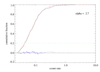
Figure 3.: Best-fit examples of statistical flare simulations for different power-law distributions. Only emission exceeding ‘quiescent’ level has been modeled. Left: Simulated light curve (extract, unnormalized). Right: Cumulative flux distribution for data (black) and model (red), and difference (blue dotted). The maximum difference (blue vertical bar) is relevant for the KS statistic. Top: Optimum case; $\alpha=2.3$ (statistical confidence: 98.2%). Middle: Too hard distribution with $\alpha=1.8$ (statistical confidence for best case: 11.7%). Bottom: Too soft distribution with $\alpha=2.7$ (statistical confidence for best case: 84.9%).

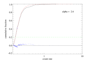
Figure 4.: Similar to Fig. 3, but all emission, including quiescent emission, has been modeled. Top: Optimum case; $\alpha=2.2$ (statistical confidence: 91.8%). Middle: Too hard distribution with $\alpha=2.1$ (statistical confidence for best case: 86.6%). Bottom: Too soft distribution with $\alpha=2.6$ (statistical confidence for best case: 53.1%).

The left panels show the first 500 bins of the simulated light curves, while the right panels show the cumulative distributions of count rates attained for the observation (black, solid) and the simulation (red, dashed). We do not use the lowest 10% of the distribution since those flux levels may be influenced by slowly varying emission in the ‘quiescent’ emission. The vertical differences between the simulated and the observed distribution are indicated dotted (blue) around the zero level: deviations to positive values indicate a locally too soft simulated distribution, negative deviations indicate locally too hard simulated distributions. The maximum deviation is indicated by a blue vertical bar. The (green) dashed horizontal line indicates the lower threshold for identifying the maximum vertical difference.

Since the last segment in the EUVE DS light curve suffered from incursion into the DS dead spot and from elevated particle radiation, we omitted that segment in our analysis. We plot in Fig. 5 the best results for different $\alpha$ values, for three cases: (i) Modeling of the EUVE DS emission above the ‘quiescent’ level (A); (ii) modeling of the complete EUVE DS emission (B); (iii) modeling the complete BeppoSAX LECS light curve (C). Acceptable models ($>$90% confidence) are found for $\alpha=2.2-2.5$.

Figure 5.: KS confidence values for different $\alpha$, using those flare rates that produce the highest confidence values for a given $\alpha$ (for the hypothesis that the simulations and the observation are drawn from the same distribution). (A): EUVE DS, emission above quiescent level. (B): EUVE DS, all emission. (C): BeppoSAX LECS, all emission.

3.2. Effect of Weak Flares

The high time-resolution of the EUV events ($\sim 1ms$) also affords the possibility of detecting weaker flares in the light-curve (see Kashyap et al. 2000). By comparing the distribution of photon arrival-time differences in the data stream with that expected from a model of flare distributions with specific power-law indices, we can account for the weak (but numerous) flares that contribute to the emission. Specifically, we

• adopt a power-law flare-distribution model (Equation 1) described by the power-law index $\alpha$ and the normalization $N_{f}$, and generate a high-time-resolution light-curve via Monte-Carlo simulation;

• add a constant component $N_{b}$ to the flare light-curve to account for true steady emission, flare emission too weak to be distinguished from steady emission, and background;

• obtain a set of event times from the model light curve;

• compare the observed distribution of arrival-time differences with that derived from the generated model event-times and compute a test statistic similar to $\chi^{2}_{r}$; and

• carry out the comparison over a grid of parameter values ($\alpha$, $N_{f}$, $N_{b}$) to find the best-fit and confidence range.

We have run the above algorithm on the first half of segment II of the AD Leo EUVE observation (see Figure 1) and find that $\alpha=2.1\pm 0.05$, a smaller value than found above, but yet $>2$. These data are clearly dominated by the large flare; an analysis of longer segments, which is expected to reduce the bias due to this flare and provide a more realistic assessment of the value of $\alpha$, is in progress.

4. Discussion and Conclusions

The analysis performed so far on EUVE light curves (Audard et al. 1999; 2000; also Kashyap et al. 2000) and the new results presented here suggest a distribution of flare energies according to a power law with a steep index: $\alpha\approx 2-3$. If the flare rate distribution continues down to levels of average solar flares, then the complete stellar corona could be heated solely by the energy released in statistical flares.

The results suggest values of $\alpha\approx 2.1-2.5$ independent of whether only the detected flares are investigated, or whether the complete emission is simulated. This suggests that (i) the extrapolation of the flare distribution to undetected flare energy levels could add large amounts of emission, and (ii) that the complete statistical distribution of count rate levels is indeed compatible with such a distribution. The two points require a lower threshold for the power-law flare distribution to confine the emission to the observed level. This has implicitly been taken into account as our simulated power-law distributions contain flares only with energies above a pre-set lower threshold. The value of the latter is determined by the normalization to the observation.

Flares could then also explain why the temperatures of active stars become increasingly hotter with ‘increasing activity’: The higher flare rate keeps more (high-density) plasma at hot temperatures, and thus the hotter plasma increasingly dominates the X-ray emission (Güdel 1997; Audard et al. 2000).

Acknowledgments.

We thank the CEA/EUVE, VLA, and BeppoSAX staff for their efforts to coordinate these observations. M. A. acknowledges support from the Swiss National Science Foundation, grants 2100-049343 and 2000-058827. The National Radio Astronomy Observatory is a facility of the National Science Foundation operated under cooperative agreement by Associated Universities, Inc. SRON is financially supported by the Netherlands Organization for Scientific Research (NWO).

References

Audard, M., Güdel, M., & Guinan, E. F. 1999, ApJ, 513, L53

Audard, M., Güdel, M., Drake, J. J., & Kashyap, V. L. 2000, ApJ, 541, 396

Antonucci, E., et al. 1984, ApJ, 413, 786

Benz, A.O., & Güdel, M. 1994, A&A, 285, 621

Collura, A., Pasquini, L., & Schmitt, J. H. M. M. 1988, A&A, 205, 197

Doyle, J. G., & Butler, C. J. 1985, Nature, 313, 378

Güdel, M. 1994, ApJS, 90, 743

Güdel, M. 1997, ApJ, 480, L121

Güdel, M., Benz, A. O. 1993, ApJ, 405, L63

Güdel, M., Guinan, E. F., & Skinner, S. L. 1997, ApJ, 483, 947

Güdel, M., et al. 2000a, ApJ, in preparation

Güdel, M., Audard, M., Guinan, E. F., Mewe, R., Drake, J. J., & Alekseev, I. Y. 2000b, in Eleventh Workshop on Cool Stars, Stellar Systems, and the Sun. ed. R. J. Garc a López, R. Rebolo, & M. R. Zapatero Osorio (San Francisco: ASP), in press

Kashyap, V. L., Drake, J. J., Audard, M., & Güdel, M. 2000, Bull. AAS 196, #13.05

Kopp, R. A., & Poletto, G. 1993, ApJ, 418, 496

Krucker, S., & Benz, A. O. 1998, ApJ, 501, L213

Lin, R. P., Schwartz, R. A., Kane, S. R., Pelling, R. M., & Hurley, K. 1984, ApJ, 283, 421

Osten, R. A., & Brown, A. 1999, ApJ, 515, 746

Parker, E. N. 1988, ApJ, 330, 474

Robinson, R. D., Carpenter, K. G., Percival, J. W., & Bookbinder, J. A. 1995, ApJ, 451, 795

Wood, B. E., Harper, G. M., Linsky, J. L., & Dempsey, R. C. 1996, ApJ, 458, 761