Neutrino Astrophysics

Abstract

A general overview of neutrino physics and astrophysics is given, starting with a historical account of the development of our understanding of neutrinos and how they helped to unravel the structure of the Standard Model. We discuss why it is so important to establish if neutrinos are massive and introduce the main scenarios to provide them a mass. The present bounds and the positive indications in favor of non-zero neutrino masses are discussed, including the recent results on atmospheric and solar neutrinos. The major role that neutrinos play in astrophysics and cosmology is illustrated.

Keywords: Neutrino astrophysics

PACS numbers:

1 The neutrino story:

1.1 The hypothetical particle:

One may trace back the appearance of neutrinos in physics to the discovery of radioactivity by Becquerel one century ago. When the energy of the electrons (beta rays) emitted in a radioactive decay was measured by Chadwick in 1914, it turned out to his surprise to be continuously distributed. This was not to be expected if the underlying process in the beta decay was the transmutation of an element $X$ into another one $X^{\prime}$ with the emission of an electron, i.e. $X\to X^{\prime}+e$, since in that case the electron should be monochromatic. The situation was so puzzling that Bohr even suggested that the conservation of energy may not hold in the weak decays. Another serious problem with the ‘nuclear models’ of the time was the belief that nuclei consisted of protons and electrons, the only known particles by then. To explain the mass and the charge of a nucleus it was then necessary that it had $A$ protons and $A-Z$ electrons in it. For instance, a ⁴He nucleus would have 4 protons and 2 electrons. Notice that this total of six fermions would make the ⁴He nucleus to be a boson, which is correct. However, the problem arouse when this theory was applied for instance to ¹⁴N, since consisting of 14 protons and 7 electrons would make it a fermion, but the measured angular momentum of the nitrogen nucleus was $I=1$.

The solution to these two puzzles was suggested by Pauli only in 1930, in a famous letter to the ‘Radioactive Ladies and Gentlemen’ gathered in a meeting in Tubingen, where he wrote: ‘I have hit upon a desperate remedy to save the exchange theorem of statistics and the law of conservation of energy. Namely, the possibility that there could exist in nuclei electrically neutral particles, that I wish to call neutrons, which have spin 1/2 …’. These had to be not heavier than electrons and interacting not more strongly than gamma rays.

With this new paradigm, the nitrogen nucleus became ¹⁴N$=14p+7e+7`n$’, which is a boson, and a beta decay now involved the emission of two particles $X\to X^{\prime}+e+`n$’, and hence the electron spectrum was continuous. Notice that no particles were created in a weak decay, both the electron and Pauli’s neutron $`n$’ were already present in the nucleus of the element $X$, and they just came out in the decay. However, in 1932 Chadwick discovered the real ‘neutron’, with a mass similar to that of the proton and being the missing building block of the nuclei, so that a nitrogen nucleus finally became just ¹⁴N$=7p+7n$, which also had the correct bosonic statistics.

In order to account now for the beta spectrum of weak decays, Fermi called Pauli’s hypotetised particle the neutrino (small neutron), $\nu$, and furthermore suggested that the fundamental process underlying beta decay was $n\to p+e+\nu$. He wrote [1] the basic interaction by analogy with the interaction known at the time, the QED, i.e. as a vector$\times$vector current interaction:

$$H_{F}=G_{F}\int{\rm d}^{3}x[\bar{\Psi}_{p}\gamma_{\mu}\Psi_{n}][\bar{\Psi}_{e}\gamma^{\mu}\Psi_{\nu}]+h.c..$$

This interaction accounted for the continuous beta spectrum, and from the measured shape at the endpoint Fermi concluded that $m_{\nu}$ was consistent with zero and had to be small. The Fermi coupling $G_{F}$ was estimated from the observed lifetimes of radioactive elements, and armed with this Hamiltonian Bethe and Peierls [2] decided to compute the cross section for the inverse beta process, i.e. for $\bar{\nu}+p\to n+e^{+}$, which was the relevant reaction to attempt the direct detection of a neutrino. The result, $\sigma=4(G_{F}^{2}/\pi)p_{e}E_{e}\simeq 2.3\times 10^{-44}$cm${}^{2}(p_{e}E_{e}/m_{e}^{2})$ was so tiny that they concluded ‘… This meant that one obviously would never be able to see a neutrino.’. For instance, if one computes the mean free path in water (with density $n\simeq 10^{23}/$cm³) of a neutrino with energy $E_{\nu}=2.5$ MeV, typical of a weak decay, the result is $\lambda\equiv 1/n\sigma\simeq 2.5\times 10^{20}$ cm, which is $10^{7}$AU, i.e. comparable to the thickness of the Galactic disk.

It was only in 1958 that Reines and Cowan were able to prove that Bethe and Peierls had been too pessimistic, when they measured for the first time the interaction of a neutrino through the inverse beta process[3]. Their strategy was essentially that, if one needs $10^{20}$ cm of water to stop a neutrino, having $10^{20}$ neutrinos a cm would be enough to stop one neutrino. Since after the second war powerful reactors started to become available, and taking into account that in every fission of an uranium nucleus the neutron rich fragments beta decay producing typically 6 $\bar{\nu}$ and liberating $\sim 200$ MeV, it is easy to show that the (isotropic) neutrino flux at a reactor is

$${d\Phi_{\nu}\over d\Omega}\simeq{2\times 10^{20}\over 4\pi}\left({{\rm Power\over GWatt}}\right){\bar{\nu}\over strad}.$$

Hence, placing a few hundred liters of water (with some Cadmium in it) near a reactor they were able to see the production of positrons (through the two 511 keV $\gamma$ produced in their annihilation with electrons) and neutrons (through the delayed $\gamma$ from the neutron capture in Cd), with a rate consistent with the expectations from the weak interactions of the neutrinos.

1.2 The vampire:

Going back in time again to follow the evolution of the theory of weak interactions of neutrinos, in 1936 Gamow and Teller [4] noticed that the $V\times V$ Hamiltonian of Fermi was probably too restrictive, and they suggested the generalization

$$H_{GT}=\sum_{i}G_{i}[\bar{p}O_{i}n][\bar{e}O^{i}\nu]+h.c.,$$

involving the operators $O_{i}=1,\ \gamma_{\mu},\ \gamma_{\mu}\gamma_{5},\ \gamma_{5},\ \sigma_{\mu\nu}$, corresponding to scalar ($S$), vector ($V$), axial vector $(A)$, pseudoscalar ($P$) and tensor ($T$) currents. However, since $A$ and $P$ only appeared here as $A\times A$ or $P\times P$, the interaction was parity conserving. The situation became unpleasant, since now there were five different coupling constants $G_{i}$ to fit with experiments, but however this step was required since some observed nuclear transitions which were forbidden for the Fermi interaction became now allowed with its generalization (GT transitions).

The story became more involved when in 1956 Lee and Yang suggested that parity could be violated in weak interactions[5]. This could explain why the particles theta and tau had exactly the same mass and charge and only differed in that the first one was decaying to two pions while the second to three pions (e.g. to states with different parity). The explanation to the puzzle was that the $\Theta$ and $\tau$ were just the same particle, now known as the charged kaon, but the (weak) interaction leading to its decays violated parity.

Parity violation was confirmed the same year by Wu [6], studying the direction of emission of the electrons emitted in the beta decay of polarised ⁶⁰Co. The decay rate is proportional to $1+\alpha\vec{P}\cdot\hat{p}_{e}$. Since the Co polarization vector $\vec{P}$ is an axial vector, while the unit vector along the electron momentum $\hat{p}_{e}$ is a vector, their scalar product is a pseudoscalar and hence a non–vanishing coefficient $\alpha$ would imply parity violation. The result was that electrons preferred to be emitted in the direction opposite to $\vec{P}$, and the measured value $\alpha\simeq-0.7$ had then profound implications for the physics of weak interactions.

The generalization by Lee and Yang of the Gamow Teller Hamiltonian was

$$H_{LY}=\sum_{i}[\bar{p}O_{i}n][\bar{e}O^{i}(G_{i}+G_{i}^{\prime}\gamma_{5})\nu]+h.c..$$

Now the presence of terms such as $V\times A$ or $P\times S$ allows for parity violation, but clearly the situation became even more unpleasant since there are now 10 couplings ($G_{i}$ and $G_{i}^{\prime}$) to determine, so that some order was really called for.

Soon the bright people in the field realized that there could be a simple explanation of why parity was violated in weak interactions, the only one involving neutrinos, and this had just to do with the nature of the neutrinos. Lee and Yang, Landau and Salam [7] realized that, if the neutrino was massless, there was no need to have both neutrino chirality states in the theory, and hence the handedness of the neutrino could be the origin for the parity violation. To see this, consider the chiral projections of a fermion

$$\Psi_{L,R}\equiv{1\mp\gamma_{5}\over 2}\Psi.$$

We note that in the relativistic limit these two projections describe left and right handed helicity states (where the helicity, i.e. the spin projection in the direction of motion, is a constant of motion for a free particle), but in general an helicity eigenstate is a mixture of the two chiralities. For a massive particle, which has to move with a velocity smaller than the speed of light, it is always possible to make a boost to a system where the helicity is reversed, and hence the helicity is clearly not a Lorentz invariant while the chirality is (and hence has the desireable properties of a charge to which a gauge boson can be coupled). If we look now to the equation of motion for a Dirac particle as the one we are used to for the description of a charged massive particle such as an electron ($(i\hbox to0.0pt{/\hss}{\partial}-m)\Psi=0$), in terms of the chiral projections this equation becomes

$$i\hbox to0.0pt{/\hss}{\partial}\Psi_{L}=m\Psi_{R}$$

$$i\hbox to0.0pt{/\hss}{\partial}\Psi_{R}=m\Psi_{L}$$

and hence clearly a mass term will mix the two chiralities. However, from these equations we see that for $m=0$, as could be the case for the neutrinos, the two equations are decoupled, and one could write a consistent theory using only one of the two chiralities (which in this case would coincide with the helicity). If the Lee Yang Hamiltonian were just to depend on a single neutrino chirality, one would have then $G_{i}=\pm G_{i}^{\prime}$ and parity violation would indeed be maximal. This situation has been described by saying that neutrinos are like vampires in Dracula’s stories: if they were to look to themselves into a mirror they would be unable to see their reflected images.

The actual helicity of the neutrino was measured by Goldhaber et al. [8]. The experiment consisted in observing the $K$-electron capture in ¹⁵²Eu ($J=0$) which produced ¹⁵²Sm^∗ ($J=1$) plus a neutrino. This excited nucleus then decayed into ¹⁵²Sm ($J=0)+\gamma$. Hence the measurement of the polarization of the photon gave the required information on the helicity of the neutrino emitted initially. The conclusion was that ‘…Our results seem compatible with … 100% negative helicity for the neutrinos’, i.e. that the neutrinos are left handed particles.

This paved the road for the $V-A$ theory of weak interactions advanced by Feynman and Gell Mann, and Marshak and Soudarshan [9], which stated that weak interactions only involved vector and axial vector currents, in the combination $V-A$ which only allows the coupling to left handed fields, i.e.

$$J_{\mu}=\bar{e}_{L}\gamma_{\mu}\nu_{L}+\bar{n}_{L}\gamma_{\mu}p_{L}$$

with $H=(G_{F}/\sqrt{2})J_{\mu}^{\dagger}J^{\mu}$. This interaction also predicted the existence of purely leptonic weak charged currents, e.g. $\nu+e\to\nu+e$, to be experimentally observed much later.

The current involving nucleons is actually not exactly $\propto\gamma_{\mu}(1-\gamma_{5})$ (only the interaction at the quark level has this form), but is instead $\propto\gamma_{\mu}(g_{V}-g_{A}\gamma_{5})$. The vector coupling remains however unrenormalised ($g_{V}=1$) due to the so called conserved vector current hypothesis (CVC), which states that the vector part of the weak hadronic charged currents ($J_{\mu}^{\pm}\propto\bar{\Psi}\gamma_{\mu}\tau^{\pm}\Psi$, with $\tau^{\pm}$ the raising and lowering operators in the isospin space $\Psi^{T}=(p,n)$) together with the isovector part of the electromagnetic current (i.e. the term proportional to $\tau_{3}$ in the decomposition $J^{em}_{\mu}\propto\bar{\Psi}\gamma_{\mu}(1+\tau_{3})\Psi$) form an isospin triplet of conserved currents. On the other hand, the axial vector hadronic current is not protected from strong interaction renormalization effects and hence $g_{A}$ does not remain equal to unity. The measured value, using for instance the lifetime of the neutron, is $g_{A}=1.26$, so that at the nucleonic level the charged current weak interactions are actually “$V-1.26A$”.

With the present understanding of weak interactions, we know that the clever idea to explain parity violation as due to the non-existence of one of the neutrino chiralities (the right handed one) was completely wrong, although it lead to major advances in the theory and ultimately to the correct interaction. Today we understand that the parity violation is a property of the gauge boson (the $W$) responsible for the gauge interaction, which couples only to the left handed fields, and not due to the absence of right handed fields. For instance, in the quark sector both left and right chiralities exists, but parity is violated because the right handed fields are singlets for the weak charged currents.

1.3 The trilogy:

In 1947 the muon was discovered in cosmic rays by Anderson and Neddermeyer. This particle was just a heavier copy of the electron, and as was suggested by Pontecorvo, it also had weak interactions $\mu+p\to n+\nu$ with the same universal strength $G_{F}$. Hincks, Pontecorvo and Steinberger showed that the muon was decaying to three particles, $\mu\to e\nu\nu$, and the question arose whether the two emitted neutrinos were similar or not. It was then shown by Feinberg [10] that, assuming the two particles were of the same kind, weak interactions couldn’t be mediated by gauge bosons (an hypothesis suggested in 1938 by Klein). The reasoning was that if the two neutrinos were equal, it would be possible to join the two neutrino lines and attach a photon to the virtual charged gauge boson ($W$) or to the external legs, so as to generate a diagram for the radiative decay $\mu\to e\gamma$. The resulting branching ratio would be larger than $10^{-5}$ and was hence already excluded at that time. This was probably the first use of ‘rare decays’ to constrain the properties of new particles.

The correct explanation for the absence of the radiative decay was put forward by Lee and Yang, who suggested that the two neutrinos emitted in the muon decay had different flavour, i.e. $\mu\to e+\nu_{e}+\nu_{\mu}$, and hence it was not possible to join the two neutrino lines to draw the radiative decay diagram. This was confirmed at Brookhaven in the first accelerator neutrino experiment[11]. They used an almost pure $\bar{\nu}_{\mu}$ beam, something which can be obtained from charged pion decays, since the $V-A$ theory implies that $\Gamma(\pi\to\ell+\bar{\nu}_{\ell})\propto m_{\ell}^{2}$, i.e. this process requires a chirality flip in the final lepton line which strongly suppresses the decays $\pi\to e+\bar{\nu}_{e}$. Putting a detector in front of this beam they were able to observe the process $\bar{\nu}+p\to n+\mu^{+}$, but no production of positrons, what proved that the neutrinos produced in a weak decay in association with a muon were not the same as those produced in a beta decay (in association with an electron). Notice that although the neutrino fluxes are much smaller at accelerators than at reactors, their higher energies make their detection feasible due to the larger cross sections ($\sigma\propto E^{2}$ for $E\ll m_{p}$, and $\sigma\propto E$ for $E\hbox to0.0pt{\raise 2.0pt\hbox{$>$}\hss}{\lower 2.0pt\hbox{$\sim$}}\ m_{p}$).

In 1975 the $\tau$hird charged lepton was discovered by Perl at SLAC, and being just a heavier copy of the electron and the muon, it was concluded that a third neutrino flavour had also to exist. The direct detection of the $\tau$ neutrino has recently been anounced by the DONUT experiment at Fermilab, looking at the short $\tau$ tracks produced by the interaction of a $\nu_{\tau}$ emitted in the decay of a heavy meson (containing a $b$ quark) produced in a beam dump. Furthermore, we know today that the number of light weakly interacting neutrinos is precisely three (see below), so that the proliferation of neutrino species seems to be now under control.

1.4 The gauge theory:

As was just mentioned, Klein had suggested that the short range charged current weak interaction could be due to the exchange of a heavy charged vector boson, the $W^{\pm}$. This boson exchange would look at small momentum transfers ($Q^{2}\ll M_{W}^{2}$) as the non renormalisable four fermion interactions discussed before. If the gauge interaction is described by the Lagrangian ${\cal L}=-(g/\sqrt{2})J_{\mu}W^{\mu}+h.c.$, from the low energy limit one can identify the Fermi coupling as $G_{F}=\sqrt{2}g^{2}/(8M_{W}^{2})$. In the sixties, Glashow, Salam and Weinberg showed that it was possible to write down a unified description of electromagnetic and weak interactions with a gauge theory based in the group $SU(2)_{L}\times U(1)_{Y}$ (weak isospin $\times$ hypercharge, with the electric charge being $Q=T_{3}+Y$), which was spontaneously broken at the weak scale down to the electromagnetic $U(1)_{em}$. This (nowadays standard) model involves the three gauge bosons in the adjoint of $SU(2)$, $V_{i}^{\mu}$ (with $i=1,2,3$), and the hypercharge gauge field $B^{\mu}$, so that the starting Lagrangian is

$${\cal L}=-g\sum_{i=1}^{3}J^{i}_{\mu}V^{\mu}_{i}-g^{\prime}J^{Y}_{\mu}B^{\mu}+h.c.,$$

with $J^{i}_{\mu}\equiv\sum_{a}\bar{\Psi}_{aL}\gamma_{\mu}(\tau_{i}/2)\Psi_{aL}$. The left handed leptonic and quark isospin doublets are $\Psi^{T}=({\nu_{e}}_{L},e_{L})$ and ($u_{L},d_{L})$ for the first generation (and similar ones for the other two heavier generations) and the right handed fields are SU(2) singlets. The hypercharge current is obtained by summing over both left and right handed fermion chiralities and is $J^{Y}_{\mu}\equiv\sum_{a}Y_{a}\bar{\Psi}_{a}\gamma_{\mu}\Psi_{a}$.

After the electroweak breaking one can identify the weak charged currents with $J^{\pm}=J^{1}\pm iJ^{2}$, which couple to the $W$ boson $W^{\pm}=(V^{1}\mp iV^{2})/\sqrt{2}$, and the two neutral vector bosons $V^{3}$ and $B$ will now combine through a rotation by the weak mixing angle $\theta_{W}$ (with tg$\theta_{W}=g^{\prime}/g$), to give

$$\pmatrix{A_{\mu}\cr Z_{\mu}}=\pmatrix{{\rm c}\theta_{W}&{\rm s}\theta_{W}\cr-{\rm s}\theta_{W}&{\rm c}\theta_{W}}\pmatrix{B_{\mu}\cr V^{3}_{\mu}}.$$ (1)

We see that the broken theory has now, besides the massless photon field $A_{\mu}$, an additional neutral vector boson, the heavy $Z_{\mu}$, whose mass turns out to be related to the $W$ boson mass through $s^{2}\theta_{W}=1-(M_{W}^{2}/M_{Z}^{2})$. The electromagnetic and neutral weak currents are given by

$$J_{\mu}^{em}=J^{Y}_{\mu}+J^{3}_{\mu}$$

$$J^{0}_{\mu}=J^{3}_{\mu}-{\rm s}^{2}\theta_{W}J^{em}_{\mu},$$

with the electromagnetic coupling being $e=g\ {\rm s}\theta_{W}$.

The great success of this model came in 1973 with the experimental observation of the weak neutral currents using muon neutrino beams at CERN (Gargamelle) and Fermilab, using the elastic process $\nu_{\mu}e\to\nu_{\mu}e$. The semileptonic processes $\nu N\to\nu X$ were also studied and the comparison of neutral and charged current rates provided a measure of the weak mixing angle. From the theoretical side t’Hooft proved the renormalisability of the theory, so that the computation of radiative corrections became also meaningful.

Figure 1: Neutral and charged current contributions to neutrino lepton scattering.

The Hamiltonian for the leptonic weak interactions $\nu_{\ell}+\ell^{\prime}\to\nu_{\ell}+\ell^{\prime}$ can be obtained, using the Standard Model just presented, from the two diagrams in figure 1. In the low energy limit ($Q^{2}\ll M_{W}^{2},\ M_{Z}^{2}$), it is just given by

$$H_{\nu_{\ell}\ell^{\prime}}={G_{F}\over\sqrt{2}}[\bar{\nu}_{\ell}\gamma_{\mu}(1-\gamma_{5})\nu_{\ell}][\bar{\ell}^{\prime}\gamma^{\mu}(c_{L}P_{L}+c_{R}P_{R})\ell^{\prime}]$$

where the left and right couplings are $c_{L}=\delta_{\ell\ell^{\prime}}+s^{2}\theta_{W}-0.5$ and $c_{R}=s^{2}\theta_{W}$. The $\delta_{\ell\ell^{\prime}}$ term in $c_{L}$ is due to the charged current diagram, which clearly only appears when $\ell=\ell^{\prime}$. On the other hand, one sees that due to the $B$ component in the $Z$ boson, the weak neutral currents also couple to the charged lepton right handed chiralities (i.e. $c_{R}\neq 0$). This interaction leads to the cross section (for $E_{\nu}\gg m_{\ell^{\prime}}$)

$$\sigma(\nu+\ell\to\nu+\ell)={2G_{F}^{2}\over\pi}m_{\ell}E_{\nu}\left[c_{L}^{2}+{c_{R}^{2}\over 3}\right],$$

and a similar expression with $c_{L}\leftrightarrow c_{R}$ for antineutrinos. Hence, we have the following relations for the neutrino elastic scatterings off electrons

$$\sigma(\nu_{e}e)\simeq 9\times 10^{-44}{\rm cm}^{2}\left({E_{\nu}\over 10\ {\rm MeV}}\right)\simeq 2.5\sigma(\bar{\nu}_{e}e)\simeq 6\sigma(\nu_{\mu,\tau}e)\simeq 7\sigma(\bar{\nu}_{\mu,\tau}e).$$

Regarding the angular distribution of the electron momentum with respect to the incident neutrino direction, in the center of mass system of the process $d\sigma(\nu_{e}e)/d\cos\theta\propto 1+0.1[(1+\cos\theta)/2]^{2}$, and it is hence almost isotropic. However, due to the boost to the laboratory system, there will be a significant correlation between the neutrino and electron momenta for $E_{\nu}\gg$MeV, and this actually allows to do astronomy with neutrinos. For instance, water cherenkov detectors such as Superkamiokande detect solar neutrinos using this process, and have been able to reconstruct a picture of the Sun with neutrinos. It will turn also to be relevant for the study of neutrino oscillations that these kind of detectors are six times more sensitive to electron type neutrinos than to the other two neutrino flavours.

Considering now the neutrino nucleon interactions, one has at low energies (1 MeV$<E_{\nu}<50$ MeV)

$$\sigma(\nu_{e}n\to pe)\simeq\sigma(\bar{\nu}_{e}p\to ne^{+})\simeq{G_{F}^{2}\over\pi}{\rm c}^{2}\theta_{C}(g_{V}^{2}+3g_{A}^{2})E_{\nu}^{2},$$

where we have now introduced the Cabibbo mixing angle $\theta_{C}$ which relates, if we ignore the third family, the quark flavour eigenstates $q^{0}$ to the mass eigenstates $q$, i.e. $d^{0}={\rm c}\theta_{C}d+{\rm s}\theta_{C}s$ and $s^{0}=-{\rm s}\theta_{C}d+{\rm c}\theta_{C}s$ (choosing a flavour basis so that the up type quark flavour and mass eigenstates coincide).

Figure 2: Neutrino nucleon and neutrino lepton cross sections (the three lines correspond, from top to bottom, to the $\nu_{e},\ \bar{\nu}_{e}$ and $\nu_{\mu,\tau}$ cross sections with electrons).

At $E_{\nu}\hbox to0.0pt{\raise 2.0pt\hbox{$>$}\hss}{\lower 2.0pt\hbox{$\sim$}}\ 50$ MeV, the nucleon no longer looks like a point-like object for the neutrinos, and hence the vector ($v_{\mu}$) and axial ($a_{\mu}$) hadronic currents involve now momentum dependent form factors, i.e.

$$\langle N(p^{\prime})|v_{\mu}|N(p)\rangle=\bar{u}(p^{\prime})[\gamma_{\mu}F_{V}+{i\over 2m_{N}}\sigma_{\mu\nu}q^{\nu}F_{W}]u(p)$$

$$\langle N(p^{\prime})|a_{\mu}|N(p)\rangle=\bar{u}(p^{\prime})[\gamma_{\mu}\gamma_{5}F_{A}+{\gamma_{5}\over 2m_{N}}q_{\mu}F_{P}]u(p),$$

where $F_{V}(q^{2})$ can be measured using electromagnetic processes and the CVC relation $F_{V}=F_{V}^{em,p}-F_{V}^{em,n}$ (i.e. as the difference between the proton and neutron electromagnetic vector form factors). Clearly $F_{V}(0)=1$ and $F_{A}(0)=1.26$, while $F_{W}$ is related to the magnetic moments of the nucleons. The $q^{2}$ dependence has the effect of significantly flattening the cross section. In the deep inelastic regime, $E_{\nu}\hbox to0.0pt{\raise 2.0pt\hbox{$>$}\hss}{\lower 2.0pt\hbox{$\sim$}}\$GeV, the neutrinos interact directly with the quark constituents. The cross section in this regime grows linearly with energy, and this provided an important test of the parton model. The main characteristics of the neutrino cross section just discussed are depicted in figure 2. For even larger energies, the gauge boson propagators enter into the play (e.g. $1/M_{W}^{2}\to 1/q^{2}$) and the growth of the cross section is less pronounced above 10 TeV ($\sigma\propto E^{0.36}$).

The most important test of the standard model came with the direct production of the $W^{\pm}$ and $Z$ gauge bosons at CERN in 1984, and with the precision measurements achieved with the $Z$ factories LEP and SLC after 1989. These $e^{+}e^{-}$ colliders working at and around the $Z$ resonance ($s=M_{Z}^{2}=($91 GeV$)^{2}$) turned out to be also crucial for neutrino physics, since studying the shape of the $e^{+}e^{-}\to f\bar{f}$ cross section near the resonance, which has the Breit–Wigner form

$$\sigma\simeq{12\pi\Gamma_{e}\Gamma_{f}\over M_{Z}^{2}}{s\over(s-M_{Z}^{2})^{2}+M_{Z}^{2}\Gamma_{Z}^{2}},$$

it becomes possible to determine the total $Z$ width $\Gamma_{Z}$. This width is just the sum of all possible partial widths, i.e.

$$\Gamma_{Z}=\sum_{f}\Gamma_{Z\to f\bar{f}}=\Gamma_{vis}+\Gamma_{inv}.$$

The visible (i.e. involving charged leptons and quarks) width $\Gamma_{vis}$ can be measured directly, and hence one can infer a value for the invisible width $\Gamma_{inv}$. Since in the standard model this last arises from the decays $Z\to\nu_{i}\bar{\nu}_{i}$, whose expected rate for decays into a given neutrino flavour is $\Gamma_{Z\to\nu\bar{\nu}}^{th}=167$ MeV, one can finally obtain the number of neutrinos coupling to the $Z$ as $N_{\nu}=\Gamma_{inv}/\Gamma_{Z\to\nu\bar{\nu}}^{th}$. The present best value for this quantity is $N_{\nu}=2.9835\pm 0.0083$, giving then a strong support to the three generation standard model.

Going through the history of the neutrinos we have seen that they have been extremely useful to understand the standard model. On the contrary, the standard model is of little help to understand the neutrinos. Since in the standard model there is no need for $\nu_{R}$, neutrinos are massless in this theory. There is however no deep principle behind this (unlike the masslessness of the photon which is protected by the electromagnetic gauge symmetry), and indeed in many extensions of the standard model neutrinos turn out to be massive. This makes the search for non-zero neutrino masses a very important issue, since it provides a window to look for physics beyond the standard model. There are many other important questions concerning the neutrinos which are not addressed by the standard model, such as whether they are Dirac or Majorana particles, whether lepton number is conserved, if the neutrino flavours are mixed (like the quarks through the Cabibbo Kobayashi Maskawa matrix) and hence oscillate when they propagate, as many hints suggest today, whether they have magnetic moments, if they decay, if they violate CP, and so on. In conclusion, although in the standard model neutrinos are a little bit boring, many of its extensions contemplate new possibilities which make the neutrino physics a very exciting field.

2 Neutrino masses:

2.1 Dirac or Majorana?

In the standard model, charged leptons (and also quarks) get their masses through their Yukawa couplings to the Higgs doublet field $\phi^{T}=(\phi_{0},\phi_{-})$

$$-{\cal L}_{Y}=\lambda\bar{L}\phi^{*}\ell_{R}+h.c.\ ,$$

where $L^{T}=(\nu,\ell)_{L}$ is a lepton doublet and $\ell_{R}$ an SU(2) singlet field. When the electroweak symmetry gets broken by the vacuum expectation value of the neutral component of the Higgs field $\langle\phi_{0}\rangle=v/\sqrt{2}$ (with $v=246$ GeV), the following ‘Dirac’ mass term results

$$-{\cal L}_{m}=m_{\ell}(\bar{\ell}_{L}\ell_{R}+\bar{\ell}_{R}\ell_{L})=m_{\ell}\bar{\ell}\ell,$$

where $m_{\ell}=\lambda v/\sqrt{2}$ and $\ell=\ell_{L}+\ell_{R}$ is the Dirac spinor field. This mass term is clearly invariant under the $U(1)$ transformation $\ell\to{\rm exp}(i\alpha)\ell$, which corresponds to the lepton number (and actually in this case also to the electromagnetic gauge invariance). From the observed fermion masses, one concludes that the Yukawa couplings range from $\lambda_{t}\simeq 1$ for the top quark up to $\lambda_{e}\simeq 10^{-5}$ for the electron.

Notice that the mass terms always couple fields with opposite chiralities, i.e. requires a $L\leftrightarrow R$ transition. Since in the standard model the right handed neutrinos are not introduced, it is not possible to write a Dirac mass term, and hence the neutrino results massless. Clearly the simplest way to give the neutrino a mass would be to introduce the right handed fields just for this purpose (having no gauge interactions, these sterile states would be essentially undetectable and unproduceable). Although this is a logical possibility, it has the ugly feature that in order to get reasonable neutrino masses, below the eV, would require unnaturally small Yukawa couplings ($\lambda_{\nu}<10^{-11}$). Fortunately it turns out that neutrinos are also very special particles in that, being neutral, there are other ways to provide them a mass. Furthermore, in some scenarios it becomes also possible to get a natural understanding of why neutrino masses are so much smaller than the charged fermion masses.

The new idea is that the left handed neutrino field actually involves two degrees of freedom, the left handed neutrino associated with the positive beta decay (i.e. emitted in association with a positron) and the other one being the right handed ‘anti’-neutrino emitted in the negative beta decays (i.e. emitted in association with an electron). It may then be possible to write down a mass term using just these two degrees of freedom and involving the required $L\leftrightarrow R$ transition. This possibility was first suggested by Majorana in 1937, in a paper named ‘Symmetric theory of the electron and positron’, and devoted mainly to the problem of getting rid of the negative energy sea of the Dirac equation[12]. As a side product, he found that for neutral particles there was ‘no more any reason to presume the existence of antiparticles’, and that ‘it was possible to modify the theory of beta emission, both positive and negative, so that it came always associated with the emission of a neutrino’. The spinor field associated to this formalism was then named in his honor a Majorana spinor.

To see how this works it is necessary to introduce the so called antiparticle field, $\psi^{c}\equiv C\bar{\psi}^{T}=C\gamma_{0}^{T}\psi^{*}$. The charge conjugation matrix $C$ has to satisfy $C\gamma_{\mu}C^{-1}=-\gamma_{\mu}^{T}$, so that for instance the Dirac equation for a charged fermion in the presence of an electromagnetic field, $(i\hbox to0.0pt{/\hss}{\partial}-e\hbox to0.0pt{/\hss}{A}-m)\psi=0$ implies that $(i\hbox to0.0pt{/\hss}{\partial}+e\hbox to0.0pt{/\hss}{A}-m)\psi^{c}=0$, i.e. that the antiparticle field has opposite charges as the particle field and the same mass. Since for a chiral projection one can show that $(\psi_{L})^{c}=(P_{L}\psi)^{c}=P_{R}\psi^{c}=(\psi^{c})_{R}$, i.e. this conjugation changes the chirality of the field, one has that $\psi^{c}$ is related to the $CP$ conjugate of $\psi$. Notice that $(\psi_{L})^{c}$ describes exactly the same two degrees of freedom described by $\psi_{L}$, but somehow using a $CP$ reflected formalism. For instance for the neutrinos, the $\nu_{L}$ operator annihilates the left handed neutrino and creates the right handed antineutrino, while the $(\nu_{L})^{c}$ operator annihilates the right handed antineutrino and creates the left handed neutrino.

We can then now write the advertised Majorana mass term, as

$$-{\cal L}_{M}={1\over 2}m[\overline{\nu_{L}}(\nu_{L})^{c}+\overline{(\nu_{L})^{c}}\nu_{L}].$$

This mass term has the required Lorentz structure (i.e. the $L\leftrightarrow R$ transition) but one can see that it does not preserve any $U(1)$ phase symmetry, i.e. it violates the so called lepton number by two units. If we introduce the Majorana field $\nu\equiv\nu_{L}+(\nu_{L})^{c}$, which under conjugation transforms into itself ($\nu^{c}=\nu$), the mass term becomes just ${\cal L}_{M}=-m\bar{\nu}\nu/2$.

Figure 3: Example of loop diagram leading to a Majorana mass term in supersymmetric models with broken $R$ parity.

Up to now we have introduced the Majorana mass by hand, contrary to the case of the charged fermions where it arose from a Yukawa coupling in a spontaneously broken theory. To follow the same procedure with the neutrinos presents however a difficulty, because the standard model neutrinos belong to $SU(2)$ doublets, and hence to write an electroweak singlet Yukawa coupling it is necessary to introduce an $SU(2)$ triplet Higgs field $\vec{\Delta}$ (something which is not particularly attractive). The coupling ${\cal L}\propto\overline{L^{c}}\vec{\sigma}L\cdot\vec{\Delta}$ would then lead to the Majorana mass term after the neutral component of the scalar gets a VEV. Alternatively, the Majorana mass term could be a loop effect in models where the neutrinos have lepton number violating couplings to new scalars, as in the so-called Zee models or in the supersymmetric models with $R$ parity violation (as illustrated in figure 3). These models have as interesting features that the masses are naturally suppressed by the loop, and they are attractive also if one looks for scenarios where the neutrinos have relatively large dipole moments, since a photon can be attached to the charged particles in the loop.

However, by far the nicest possibility to give neutrinos a mass is the so-called see-saw model introduced by Gell Man, Ramond and Slansky and by Yanagida in 1979[13]. In this scenario, which naturally occurs in grand unified models such as $SO(10)$, one introduces the $SU(2)$ singlet right handed neutrinos. One has now not only the ordinary Dirac mass term, but also a Majorana mass for the singlets which is generated by the VEV of an $SU(2)$ singlet Higgs, whose natural scale is the scale of breaking of the grand unified group, i.e. in the range $10^{12}$–$10^{16}$ GeV. Hence the Lagrangian will contain

$${\cal L}_{M}={1\over 2}\overline{(\nu_{L},(N_{R})^{c})}\pmatrix{0&m_{D}\cr m_{D}&M}\pmatrix{(\nu_{L})^{c}\cr N_{R}}+h.c..$$

The mass eigenstates are two Majorana fields with masses $m_{light}\simeq m_{D}^{2}/M$ and $m_{heavy}\simeq M$. Since $m_{D}/M\ll 1$, we see that $m_{light}\ll m_{D}$, and hence the lightness of the known neutrinos is here related to the heaviness of the sterile states $N_{R}$, as figure 4 illustrates.

Figure 4: The see-saw model: pushing one mass up brings the other down.

If we actually introduce one singlet neutrino per family, the mass terms in eq. (2.1) are $3\times 3$ matrices. Notice that if $m_{D}$ is similar to the up-type quark masses, as happens in $SO(10)$, one would have $m_{\nu_{\tau}}\sim m_{t}^{2}/M\simeq 4$ eV$(10^{13}$ GeV/$M$). It is clear then that in these scenarios the observation of neutrino masses below the eV would point out to new physics at about the GUT scale.

2.2 The quest for the neutrino mass:

Already in his original paper on the theory of weak interactions Fermi had noticed that the observed shape of the electron spectrum was suggesting a small mass for the neutrino. The sensitivity to $m_{\nu_{e}}$ in the decay $X\to X^{\prime}+e+\bar{\nu}_{e}$ arises clearly because the larger $m_{\nu}$, the less available kinetic energy remains for the decay products, and hence the maximum electron energy is reduced. To see this consider the phase space factor of the decay, $d\Gamma\propto d^{3}p_{e}d^{3}p_{\nu}\propto p_{e}E_{e}dE_{e}p_{\nu}E_{\nu}dE_{\nu}\delta(E_{e}+E_{\nu}-Q)$, with the $Q$–value being the total available energy in the decay: $Q\simeq M_{X}-M_{X^{\prime}}-m_{e}$. This leads to a differential electron spectrum proportional to $d\Gamma/dE_{e}\propto p_{e}E_{e}(Q-E_{e})\sqrt{(Q-E_{e})^{2}-m_{\nu}^{2}}$, whose shape near the endpoint ($E_{e}\simeq Q-m_{\nu}$) depends on $m_{\nu}$ (actually the slope becomes infinite at the endpoint for $m_{\nu}\neq 0$, while it vanishes for $m_{\nu}=0$).

Since the fraction of events in an interval $\Delta E_{e}$ around the endpoint is $\sim(\Delta E_{e}/Q)^{3}$, to enhance the sensitivity to the neutrino mass it is better to use processes with small $Q$-values, what makes the tritium the most sensitive nucleus ($Q=18.6$ keV). Recent experiments at Mainz and Troitsk have allowed to set the bound $m_{\nu_{e}}\leq 2.2$ eV[15], finally overcoming the previous situation in which the results were giving systematically an unphysical negative value for $m_{\nu_{e}}^{2}$, corresponding to a small electron excess near the endpoint. To improve this bound is quite hard because the fraction of events within say 10 eV of the endpoint is already $\sim 10^{-10}$.

Regarding the muon neutrino, a direct bound on its mass can be set by looking to its effects on the available energy for the muon in the decay of a pion at rest, $\pi^{+}\to\mu^{+}+\nu_{\mu}$. From the knowledge of the $\pi$ and $\mu$ masses, and measuring the momentum of the monochromatic muon, one can get the neutrino mass through the relation

$$m^{2}_{\nu_{\mu}}=m^{2}_{\pi}+m^{2}_{\mu}-2m_{\pi}\sqrt{p^{2}_{\mu}+m^{2}_{\mu}}.$$

The best bounds at present are $m_{\nu_{\mu}}\leq 170$ keV from PSI, and again they are difficult to improve through this process since the neutrino mass comes from the difference of two large quantities. There is however a proposal to use the muon $(g-2)$ experiment at BNL to become sensitive down to $m_{\nu_{\mu}}\leq 8$ keV.

Finally, the bound on the $\nu_{\tau}$ mass is $m_{\nu_{\tau}}\leq 17$ MeV and comes from the effects it has on the available phase space of the pions in the decay $\tau\to 5\pi+\nu_{\tau}$ measured at LEP.

To look for the electron neutrino mass, besides the endpoint of the ordinary beta decay there is another interesting process, but which is however only sensitive to a Majorana (lepton number violating) mass. This is the so called double beta decay. Some nuclei can undergo transitions in which two beta decays take place simultaneously, with the emission of two electrons and two antineutrinos ($2\beta 2\nu$ in fig. 5). These transitions have been observed in a few isotopes (⁸²Se, ⁷⁶Ge, ¹⁰⁰Mo, ¹¹⁶Cd, ¹⁵⁰Nd) in which the single beta decay is forbidden, and the associated lifetimes are huge ($10^{19}$–$10^{24}$ yr). However, if the neutrino were a Majorana particle, the virtual antineutrino emitted in one vertex could flip chirality by a mass insertion and be absorbed in the second vertex as a neutrino, as exemplified in fig. 5 ($2\beta 0\nu$). In this way only two electrons would be emitted and this could be observed as a monochromatic line in the added spectrum of the two electrons. The non observation of this effect has allowed to set the bound $m_{\nu_{e}}^{Maj}\leq 0.3$ eV (by the Heidelberg–Moscow collaboration at Gran Sasso). There are projects to improve the sensitivity of $2\beta 0\nu$ down to $m_{\nu_{e}}\sim 10^{-2}$ eV, and we note that this bound is quite relevant since as we have seen, if neutrinos are indeed massive it is somehow theoretically favored (e.g. in the see saw models) that they are Majorana particles.

Figure 5: Double beta decay with and without neutrino emission, and qualitative shape of the expected added spectrum of the two electrons.

At this point it is important to extend the discussion to take into account that there are three generations of neutrinos. If neutrinos turn out to be massive, there is no reason to expect that the mass eigenstates ($\nu_{k}$, with $k=1,2,3$) would coincide with the flavour (gauge) eigenstates ($\nu_{\alpha}$, with $\alpha=e,\mu,\tau$), and hence, in the same way that quark states are mixed through the Cabibbo, Kobayashi and Maskawa matrix, neutrinos would be related through the Maki, Nakagawa and Sakita mixing matrix [14], i.e. $\nu_{\alpha}=V_{\alpha k}\nu_{k}$. The MNS matrix can be parametrized as ($c_{12}\equiv\cos\theta_{12}$, etc.)

$$V=\pmatrix{c_{12}c_{13}&c_{13}s_{12}&s_{13}\cr-c_{23}s_{12}e^{i\delta}-c_{12}s_{13}s_{23}&c_{12}c_{23}e^{i\delta}-s_{12}s_{13}s_{23}&c_{13}s_{23}\cr s_{23}s_{12}e^{i\delta}-c_{12}c_{23}s_{13}&-c_{12}s_{23}e^{i\delta}-c_{23}s_{12}s_{13}&c_{13}c_{23}}\pmatrix{e^{i\alpha}&0&0\cr 0&e^{i\beta}&0\cr 0&0&1}$$

When the electron neutrino is a mixture of mass eigenstates, the $2\beta 0\nu$ decay amplitude will be proportional now to an ‘effective electron neutrino mass’ $\langle m_{\nu_{e}}\rangle=V_{ek}^{2}m_{k}$, where here we adopted the Majorana neutrino fields as self-conjugates ($\chi_{k}^{c}=\chi_{k}$). If one allows for Majorana creation phases in the fields, $\chi_{k}^{c}=e^{i\alpha_{k}}\chi_{k}$, these phases will appear in the effective mass, $\langle m_{\nu_{e}}\rangle={V^{\prime}_{ek}}^{2}e^{i\alpha_{k}}m_{k}$. Clearly $\langle m_{\nu_{e}}\rangle$ has to be independent of the unphysical phases $\alpha_{k}$, so that the matrix diagonalising the mass matrix in the new basis has to change accordingly, i. e. $V^{\prime}_{ek}=e^{-i\alpha_{k}/2}V_{ek}$. In particular, $\alpha$ and $\beta$ may be removed from $V$ in this way, but they would anyhow reappear at the end in $\langle m\rangle$ through the propagators of the Majorana fields, which depend on the creation phases. When CP is conserved, it is sometimes considered convenient to choose basis so that $V_{ek}$ is real (i.e. $\delta=0$ from CP conservation and $\alpha$ and $\beta$ are reabsorbed in the Majorana creation phases of the fields). In this case each contribution to $\langle m\rangle$ turns out to be multiplied by the intrinsic CP-parity of the mass eigenstate, $\langle m_{\nu_{e}}\rangle=|\sum_{k}|V_{ek}|^{2}\eta_{CP}(\chi_{k})m_{k}|$, with $\eta_{CP}=\pm i$. States with opposite CP parities can then induce cancellations in $2\beta 0\nu$ decays.

Double beta decay is the only process sensitive to the phases $\alpha$ and $\beta$. These phases can be just phased away for Dirac neutrinos, and hence in all experiments (such as oscillations) where it is not possible to distinguish between Majorana and Dirac neutrinos, it is not possible to measure them. However, oscillation experiments are the most sensitive way to measure small neutrino masses and their mixing angles, as we now turn to discuss.

2.3 Neutrino oscillations:

The possibility that neutrino flavour eigenstates be a superposition of mass eigenstates, as was just discussed, allows for the phenomenon of neutrino oscillations. This is a quantum mechanical interference effect (and as such it is sensitive to quite small masses) and arises because different mass eigenstates propagate differently, and hence the flavor composition of a state can change with time.

To see this consider a flavour eigenstate neutrino $\nu_{\alpha}$ with momentum $p$ produced at time $t=0$ (e.g. a $\nu_{\mu}$ produced in the decay $\pi^{+}\to\mu^{+}+\nu_{\mu}$). The initial state is then

$$|\nu_{\alpha}\rangle=\sum_{k}V_{\alpha k}|\nu_{k}\rangle.$$

We know that the mass eigenstates evolve with time according to $|\nu_{k}(t,x)\rangle={\rm exp}[i(px-E_{k}t)]|\nu_{k}\rangle$. In the relativistic limit relevant for neutrinos, one has that $E_{k}=\sqrt{p^{2}+m_{k}^{2}}\simeq p+m^{2}_{k}/2E$, and thus the different mass eigenstates will acquire different phases as they propagate. Hence, the probability of observing a flavour $\nu_{\beta}$ at time $t$ is just

$$P(\nu_{\alpha}\to\nu_{\beta})=|\langle\nu_{\beta}|\nu(t)\rangle|^{2}=|\sum_{k}V_{\alpha k}e^{-i{m_{i}^{2}\over 2E}t}V^{*}_{\beta k}|^{2}.$$

In the case of two generations, taking $V$ just as a rotation with mixing angle $\theta$, one has

$$P(\nu_{\alpha}\to\nu_{\beta})=\sin^{2}2\theta\ \sin^{2}\left({\Delta m^{2}x\over 4E}\right),$$

which depends on the squared mass difference $\Delta m^{2}=m_{2}^{2}-m_{1}^{2}$, since this is what gives the phase difference in the propagation of the mass eigenstates. Hence, the amplitude of the flavour oscillations is given by $\sin^{2}2\theta$ and the oscillation length of the modulation is $L_{osc}\equiv 4\pi E/\Delta m^{2}\simeq 2.5$ m $E$[MeV]/$\Delta m^{2}$[eV²]. We see then that neutrinos will typically oscillate with a macroscopic wavelength. For instance, putting a detector at $\sim 100$ m from a reactor allows to test oscillations of $\nu_{e}$’s to another flavour (or into a singlet neutrino) down to $\Delta m^{2}\sim 10^{-2}$ eV² if sin${}^{2}2\theta$ is not too small ($\geq 0.1$). The CHOOZ experiment has even reached $\Delta m^{2}\sim 10^{-3}$ eV² putting a large detector at 1 km distance, and the future KAMLAND experiment will be sensitive to reactor neutrinos arriving from $\sim 10^{2}$ km, and hence will test $\Delta m^{2}\sim 10^{-5}$ eV² in a few years (see fig. 6).

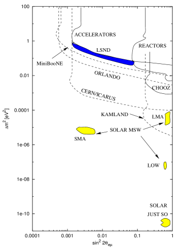
Figure 6: Present bounds (solid lines), projected sensitivities of future experiments (dashed lines) and values suggested by LSND and solar neutrino experiments for $\nu_{e}\leftrightarrow\nu_{\mu}$ oscillations.

These kind of experiments look essentially for the disappearance of the reactor $\nu_{e}$’s, i.e. to a reduction in the original $\nu_{e}$ flux. When one uses more energetic neutrinos from accelerators, it becomes possible also to study the appearance of a flavour different from the original one, with the advantage that one becomes sensitive to very small oscillation amplitudes (i.e. small sin${}^{2}2\theta$ values), since the observation of only a few events is enough to establish a positive signal. At present there is one experiment (LSND) claiming a positive signal of $\nu_{\mu}\to\nu_{e}$ conversion, suggesting the neutrino parameters in the region indicated in fig. 6, once the region excluded by other experiments is taken into account. The appearance of $\nu_{\tau}$’s out of a $\nu_{\mu}$ beam was searched at CHORUS and NOMAD at CERN without success, allowing to exclude the region indicated in fig. 7, which is a region of relevance for cosmology since neutrinos heavier than $\sim$ eV would contribute to the dark matter in the Universe significantly.

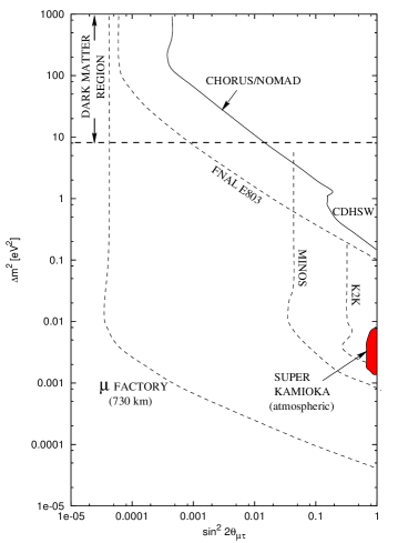
Figure 7: Present bounds (solid lines), projected sensitivities of future experiments (dashed lines) and values suggested by the atmospheric neutrino anomaly for $\nu_{\mu}\leftrightarrow\nu_{\tau}$ oscillations. Also shown is the region where neutrinos would constitute a significant fraction of the dark matter ($\Omega_{\nu}>0.1$).

In figs. 6 and 7 we also display the sensitivity of various new experiments under construction or still at the proposal level, showing that significant improvements are to be expected in the near future (a useful web page with links to the experiments is the Neutrino Industry Homepage). These new experiments will in particular allow to test some of the most clear hints we have at present in favor of massive neutrinos, which come from the two most important natural sources of neutrinos that we have: the atmospheric and the solar neutrinos.

3 Neutrinos in astrophysics and cosmology:

We have seen that neutrinos made their shy appearance in physics just by steeling a little bit of the momentum of the electrons in a beta decay. In astrophysics however, neutrinos have a major (sometimes preponderant) role, being produced copiously in several environments.

3.1 Atmospheric neutrinos:

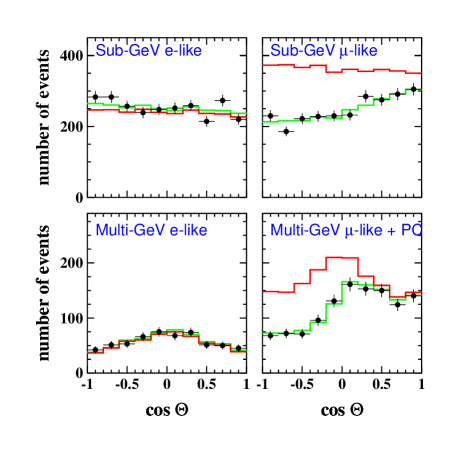
Figure 8: Distribution of the contained and partially contained event data versus cosine of the zenith angle ($\cos\theta=-1$ being up-going, while +1 being down-going) for two energy ranges, from 1144 live days of Super-Kamiokande data (from ref. [16]). The solid line corresponds to the expectations with no oscillations, while the lighter line is for $\nu_{\mu}\to\nu_{\tau}$ oscillations with maximal mixing and $\Delta m^{2}=0.003$ eV².

When a cosmic ray (proton or nucleus) hits the atmosphere and knocks a nucleus a few tens of km above ground, an hadronic (and electromagnetic) shower is initiated, in which pions in particular are copiously produced. The charged pion decays are the main source of atmospheric neutrinos through the chain $\pi\to\mu\nu_{\mu}\to e\nu_{e}\nu_{\mu}\nu_{\mu}$. One expects then twice as many $\nu_{\mu}$’s than $\nu_{e}$’s (actually at very high energies, $E_{\nu}\gg$ GeV, the parent muons may reach the ground and hence be stopped before decaying, so that the expected ratio $R\equiv(\nu_{\mu}+\bar{\nu}_{\mu})/(\nu_{e}+\bar{\nu}_{e})$ should be even larger than two at high energies). However, the observation of the atmospheric neutrinos by IMB, Kamioka, Soudan, MACRO and Super Kamiokande indicates that there is a deficit of muon neutrinos, with $R_{obs}/R_{th}\simeq 2/3$.

More remarkably, the Super Kamiokande experiment observes a zenith angle dependence indicating that neutrinos coming from above (with pathlengths $d\sim 20$ km) had not enough time to oscillate, especially in the multi-GeV sample for which the neutrino oscillation length is larger, while those from below ($d\sim 13000$ km) have already oscillated (see figure 8). The most plausible explanation for these effects is an oscillation $\nu_{\mu}\to\nu_{\tau}$ with maximal mixing and $\Delta m^{2}\simeq 2$–$7\times 10^{-3}$ eV²[16, 17], and as shown in fig. 8 the fit to the observed angular dependence is in excellent agreement with the oscillation hypothesis. Since the electron flux shape is in good agreement with the theoretical predictions, this means that the oscillations from $\nu_{\mu}\to\nu_{e}$ can not provide a satisfactory explanation for the anomaly (and furthermore they are also excluded from the negative results of the CHOOZ reactor search for oscillations). On the other hand, oscillations to sterile states would be affected by matter effects ($\nu_{\mu}$ and $\nu_{\tau}$ are equally affected by neutral current interactions when crossing the Earth, while sterile states are not), and this would modify the angular dependence of the oscillations in a way which is not favored by observations [17]. The oscillations into active states ($\nu_{\tau}$) is also favored by observables which depend on the neutral current interactions, such as the $\pi_{0}$ production in the detector or the ‘multi ring’ events [16].

An important experiment which is running now and can test the oscillation solution to the atmospheric neutrino anomaly is K2K, consisting of a beam of muon neutrinos sent from KEK to the Super-Kamiokande detector (baseline of 250 km). The first preliminary results of the initial run indicate that there is a deficit of muon neutrinos at the detector ($40.3^{+4.7}_{-4.6}$ events expected with only 27 observed), consistent with the expectations from the oscillation solution[18].

In conclusion, the atmospheric neutrinos provide the strongest signal that we have at present in favor of non-zero neutrino masses, and are hence indicating the need for physics beyond the standard model.

3.2 Solar neutrinos:

The sun gets its energy from the fusion reactions taking place in its interior, where essentially four protons combine to form a He nucleus. By charge conservation this has to be accompanied by the emission of two positrons and, by lepton number conservation in the weak processes, two $\nu_{e}$’s have to be produced. This fusion liberates 27 MeV of energy, which is eventually emitted mainly (97%) as photons and the rest (3%) as neutrinos. Knowing the energy flux of the solar radiation reaching the Earth ($k_{\odot}\simeq 1.5$ kW/m²), it is then simple to estimate that the solar neutrino flux at Earth is $\Phi_{\nu}\simeq 2k_{\odot}/27$ MeV $\simeq 6\times 10^{10}\nu_{e}/$cm²s, which is a very large number indeed.

Many experiments have looked for these solar neutrinos: the radiochemical experiments with ³⁷Cl at Homestake and with gallium at SAGE, GALLEX and GNO, and the water Cherenkov real time detectors (Super-) Kamiokande and more recently the heavy water Subdury Neutrino Observatory (SNO). The puzzling result which has been with us for the last thirty years is that only between 1/2 to 1/3 of the expected fluxes are observed. Remarkably, Pontecorvo [19] noticed even before the first observation of solar neutrinos by Davies that neutrino oscillations could reduce the expected rates. We note that the oscillation length of solar neutrinos ($E\sim 0.1$–10 MeV) is of the order of 1 AU for $\Delta m^{2}\sim 10^{-10}$ eV², and hence even those tiny neutrino masses can have observable effects if the mixing angles are large (this would be the ‘just so’ solution to the solar neutrino problem). Much more remarkable is the possibility of explaining the puzzle by resonantly enhanced oscillations of neutrinos as they propagate outwards through the Sun. Indeed, the solar medium affects $\nu_{e}$’s differently than $\nu_{\mu,\tau}$’s (since only the first interact through charged currents with the electrons present), and this modifies the oscillations in a beautiful way through an interplay of neutrino mixings and matter effects, in the so called MSW effect [20]. The magic of this effect is that large conversion probabilities can occur even for small mixing angles as the neutrinos suffer a resonant conversion when they travel through a medium with varying density. In the case of the Sun, this will happen for solar neutrinos for a wide range of masses ($\Delta m^{2}$ between $10^{-8}$ eV² and $10^{-4}$ eV²) and as the propagation is ‘adiabatic’ (i.e. for sin${}^{2}2\theta\hbox to0.0pt{\raise 2.0pt\hbox{$>$}\hss}{\lower 2.0pt\hbox{$\sim$}}\ (E/10$ MeV)$6\times 10^{-8}$ eV${}^{2}/\Delta m^{2}$), so that to get large flux suppressions is clearly not a matter of fine-tunning (see [21, 22] for reviews). The observed neutrino fluxes in the different experiments imply that the possible solutions based on this mechanism require $\Delta m^{2}\simeq 10^{-5}$ eV² with small mixings $s^{2}2\theta\simeq$ few$\times 10^{-3}$ eV² (SMA) or large mixing (LMA), or lower values of mass differences, $\Delta m^{2}\simeq 10^{-7}$ eV² with large mixing (LOW), as shown in fig. 6. Besides the overall fluxes other important tests are the measurement of the neutrino spectrum in the water Cherenkov detectors searching for spectral distortions, a day-night effect due to possible regeneration by matter effects in the Earth for the solar neutrinos entering from below (during the night) or an annual modulation of the signal (important mainly for the just-so oscillation solutions for which the oscillation length is ${\cal O}$(1 AU)) which may be observable thanks to the eccentricity of the Earth orbit around the sun, but unfortunatley none of these smoking-gun signals has yet proven to be conclussive. This year the new heavy water experiment SNO has anounced the first data and they will help with the accurate measurement of the neutrino spectrum, since the CC process $\nu_{e}+D\to p+p+e$ gives a cleaner measurement of the incident neutrino energy than the $\nu_{e}+e\to\nu_{e}+e$ process available to Super-Kamiokande. Most importantly, when the neutron detectors will be introduced to measure the NC reaction $\nu_{i}+D\to n+p+\nu_{i}$, the comparison of the charged current rates (only sensitive to $\nu_{e}$s) with the NC ones, sensitive to all neutrino flavors, will allow to test unambiguously if an oscillation to another active neutrino has occured. Also the future Borexino experiment will be crucial because it is sensitive to the neutrino lines produced by the electron capture on Be in the solar fusion reaction chain, which seem to be the most suppressed ones from the fits to existing data.

At present the experimental data slightly favors the LMA solution. This suggests, together with the atmospheric neutrino anomaly, that the mixing in the neutrino sector might be “bi-maximal” (both $\theta_{12}$ and $\theta_{23}\simeq\pi/4$), and hence with a pattern quite different from the one we know from the quark sector. This hint actually provides an important guiding principle in the search for the fundamental theory underlying the standard model of particle physics.

3.3 Supernova neutrinos:

The most spectacular neutrino fireworks in the Universe are the supernova explosions, which correspond to the death of a very massive star. In this process the inner Fe core ($M_{c}\simeq 1.4\ M_{\odot}$), unable to get pressure support gives up to the pull of gravity and collapses down to nuclear densities (few$\times 10^{14}$g/cm³), forming a very dense proto-neutron star. At this moment neutrinos become the main character on stage, and 99% of the gravitational binding energy gained (few$\times 10^{53}$ ergs) is released in a violent burst of neutrinos and antineutrinos of the three flavours, with typical energies of a few tens of MeV. Being the density so high, even the weakly interacting neutrinos become trapped in the core, and they diffuse out in a few seconds to be emitted from the so called neutrinospheres (at $\rho\sim 10^{12}$ g/cm³). These neutrino fluxes then last for $\sim 10$ s, after which the initially trapped lepton number is lost and the neutron star cools more slowly.

During those $\sim 10$ s the neutrino luminosity of the supernova ($\sim 10^{52}$ erg/s) is comparable to the total luminosity of the Universe (c.f. $L_{\odot}\simeq 4\times 10^{33}$ erg/s), but unfortunately only a couple of such events occur in our galaxy per century, so that one has to be patient. Fortunately, on February 1987 a supernova exploded in the nearby ($d\sim 50$ kpc) Large Magellanic Cloud, producing a dozen neutrino events in the Kamiokande and IMB detectors. This started extra solar system neutrino astronomy and provided a very basic proof of the explosion mechanism. With the new larger detectors under operation at present (SuperKamioka and SNO) it is expected that a future galactic supernova ($d\sim 10$ kpc) would produce several thousand neutrino events and hence allow detailed studies of the supernova physics.

Also sensitive tests of neutrino properties will be feasible if a galactic supernova is observed. The simplest example being the limits on the neutrino mass which would result from the measured burst duration as a function of the neutrino energy. Indeed, if neutrinos are massive, their velocity will be $v=c\sqrt{1-(m_{\nu}/E)^{2}}$, and hence the travel time from a SN at distance $d$ would be $t\simeq{d\over c}[1-{1\over 2}(m_{\nu}/E)^{2}]$, implying that lower energy neutrinos ($E\sim 10$ MeV) would arrive later than high energy ones by an amount $\Delta t\sim 0.5(d/10$ kpc) ($m_{\nu}/10$ eV)²s. Looking for this effect a sensitivity down to $m_{\nu_{\mu,\tau}}\sim 25$ eV would be achievable from a supernova at 10 kpc, and this is much better than the present direct bounds on the $\nu_{\mu,\tau}$ masses.

Since the matter densities at the neutrino-spheres are huge, matter effects in the supernova interior can affect neutrino oscillations for a very wide range of mass differences and mixings, making supernovae also a very interesting laboratory for oscillation studies, and in particular this may be useful for the measurement of $\theta_{13}$ (see e.g. [23]).

What remains after a (type II) supernova explosion is a pulsar, i.e. a fastly rotating magnetised neutron star. One of the mysteries related to pulsars is that they move much faster ($v\sim$ few hundred km/s) than their progenitors ($v\sim$ few tenths of km/s). There is no satisfactory standard explanation of how these initial kicks are imparted to the pulsar and here neutrinos may also have something to say. It has been suggested that these kicks could be due to a macroscopic manifestation of the parity violation of weak interactions, i.e. that in the same way as electrons preferred to be emitted in the direction opposite to the polarisation of the ⁶⁰Co nuclei in the experiment of Wu (and hence the neutrinos preferred to be emitted in the same direction), the neutrinos in the supernova explosions would be biased towards one side of the star because of the polarisation induced in the matter by the large magnetic fields present [24], leading to some kind of neutrino rocket effect, as shown in fig. 9.

Figure 9: Pulsar kicks from neutrino rockets?

Although only a 1% asymmetry in the emission of the neutrinos would be enough to explain the observed velocities, the magnetic fields required are $\sim 10^{16}$ G, much larger than the ones inferred from observations ($\sim 10^{12}$–$10^{13}$ G). An attempt has also been done [25] to exploit the fact that the neutrino oscillations in matter are affected by the magnetic field, and hence the resonant flavor conversion would take place in an off-centered surface. Since $\nu_{\tau}$’s (or $\nu_{\mu}$’s) interact less than $\nu_{e}$’s, an oscillation from $\nu_{e}\to\nu_{\tau}$ in the region where $\nu_{e}$’s are still trapped but $\nu_{\tau}$’s can freely escape would generate a $\nu_{\tau}$ flux from a deeper region of the star in one side than in the other. Hence if one assumes that the temperature profile is isotropic, neutrinos from the deeper side will be more energetic than those from the opposite side and can then be the source of the kick. This would require however $\Delta m^{2}>(100$ eV)², which is uncomfortably large, and $B>10^{14}$ G. Moreover, it has been argued [26] that the assumption of an isotropic $T$ profile near the neutrinospheres will not hold, since the side where the escaping neutrinos are more energetic will rapidly cool (the neutrinosphere region has negligible heat capacity compared to the core) adjusting the temperature gradient so that the isotropic energy flux generated in the core will manage ultimately to get out isotropically.

An asymmetric neutrino emission due to an asymmetric magnetic field affecting asymmetrically the $\nu_{e}$ opacities has also been proposed, but again the magnetic fields required are too large ($B\sim 10^{16}$ G) [27].

As a summary, to explain the pulsar kicks as due to an asymmetry in the neutrino emission is attractive theoretically, but unfortunately doesn’t seem to work. Maybe when three dimensional simulations of the explosion would become available, possibly including the presence of a binary companion, larger asymmetries would be found just from standard hydrodynamical processes.

Supernovae are also helpful for us in that they throw away into the interstellar medium all the heavy elements produced during the star’s life, which are then recycled into second generation stars like the Sun, planetary systems and so on. However, 25% of the baryonic mass of the Universe was already in the form of He nuclei well before the formation of the first stars, and as we understand now this He was formed a few seconds after the big bang in the so-called primordial nucleosynthesis. Remarkably, the production of this He also depends on the neutrinos, and the interplay between neutrino physics and primordial nucleosynthesis provided the first important astro-particle connection.

3.4 Cosmic neutrino background and primordial nucleosynthesis:

In the same way as the big bang left over the 2.7^∘K cosmic background radiation, which decoupled from matter after the recombination epoch ($T\sim$ eV), there should also be a relic background of cosmic neutrinos (C$\nu$B) left over from an earlier epoch ($T\sim$ MeV), when weakly interacting neutrinos decoupled from the $\nu_{i}$–$e$–$\gamma$ primordial soup. Slightly after the neutrino decoupling, $e^{+}e^{-}$ pairs annihilated and reheated the photons, so that the present temperature of the C$\nu$B is $T_{\nu}\simeq 1.9^{\circ}$K, slightly smaller than the photon one. This means that there should be today a density of neutrinos (and antineutrinos) of each flavour $n_{\nu_{i}}\simeq 110$ cm^-3.

Primordial nucleosynthesis occurs between $T\sim 1$ MeV and $10^{-2}$ MeV, an epoch at which the density of the Universe was dominated by radiation (photons and neutrinos). This means that the expansion rate of the Universe depended on the number of neutrino species $N_{\nu}$, becoming faster the bigger $N_{\nu}$ ($H\propto\sqrt{\rho}\propto\sqrt{\rho_{\gamma}+N_{\nu}\rho_{\nu}}$, with $\rho_{\nu}$ the density for one neutrino species). Helium production just occurred after deuterium photodissociation became inefficient at $T\sim 0.1$ MeV, with essentially all neutrons present at this time ending up into He. The crucial point is that the faster the expansion rate, the larger fraction of neutrons (with respect to protons) would have survived to produce He nuclei. This implies that an observational upper bound on the primordial He abundance will translate into an upper bound on the number of neutrino species. Actually the predictions also depend in the total amount of baryons present in the Universe ($\eta=n_{B}/n_{\gamma}$), which can be determined studying the very small amounts of primordial D and ⁷Li produced. The observational D measurements are somewhat unclear at presents, with determinations in the low side implying the strong constraint $N_{\nu}<3.3$, while those in the high side implying $N_{\nu}<4.8$ [28]. It is important that nucleosynthesis bounds on $N_{\nu}$ were established well before the LEP measurement of the number of standard neutrinos. Another interesting application of the nucleosynthesis bound on $N_{\nu}$ is that it constrains the mixing of active and sterile neutrinos since these last may be brought into equilibrium by oscillations in the early universe, and this may even exclude the atmospheric solution involving $\nu_{\mu}\to\nu_{s}$ oscillations (irrespectively of the fact that it is disfavored experimentally).

As a side product of primordial nucleosynthesis theory one can determine that the amount of baryonic matter in the Universe has to satisfy $\eta\simeq 1$–$6\times 10^{-10}$. The explanation of this small number is one of the big challenges for particle physics and another remarkable fact of neutrinos is that they might be ultimately responsible for this matter-antimatter asymmetry.

3.5 Leptogenesis:

Figure 10: One loop CP violating diagrams for leptogenesis.

The explanation of the observed baryon asymmetry as due to microphysical processes taking place in the early Universe is known to be possible provided the three Sakharov conditions are fulfilled: $i)$ the existence of baryon number violating interactions ($\hbox to0.0pt{/\hss}{B}$), $ii)$ the existence of C and CP violation ($\hbox to0.0pt{/\hss}{C}$ and $\hbox to0.0pt{\it C\hss}{\,\,\not P}$) and $iii)$ departure from chemical equilibrium ($\hbox to0.0pt{\it E\hss}{\,\,\not q}$). The simplest scenarios fulfilling these conditions appeared in the seventies with the advent of GUT theories, where heavy color triplet Higgs bosons can decay out of equilibrium in the rapidly expanding Universe (at $T\sim M_{T}\sim 10^{13}$ GeV) violating B, C and CP. In the middle of the eighties it was realized however that in the Standard Model non-perturbative $\hbox to0.0pt{/\hss}{B}$ and $\hbox to0.0pt{/\hss}{L}$ (but $B-L$ conserving) processes where in equilibrium at high temperatures $(T>100$ GeV), and would lead to a transmutation between $B$ and $L$ numbers, with the final outcome that $n_{B}\simeq n_{B-L}/3$. This was a big problem for the simplest GUTs like SU(5), where $B-L$ is conserved (and hence $n_{B-L}=0$), but it was rapidly turned into a virtue by Fukugita and Yanagida [29], who realised that it could be sufficient to generate initially a lepton number asymmetry and this will then be reprocessed into a baryon number asymmetry. The nice thing is that in see-saw models the generation of a lepton asymmetry (leptogenesis) is quite natural, since the heavy singlet Majorana neutrinos would decay out of equilibrium (at $T\hbox to0.0pt{\raise 2.0pt\hbox{$<$}\hss}{\lower 2.0pt\hbox{$\sim$}}\ M_{N}$) through $N_{R}\to\ell H,\ \bar{\ell}H^{*}$, i.e. into final states with different $L$, and the CP violation appearing at one loop through the diagrams in fig. 10 would lead [30] to $\Gamma(N\to\ell H)\neq\Gamma(N\to\bar{\ell}H^{*})$, so that a final $L$ asymmetry will result. Reasonable parameter values lead naturally to the required asymmetries ($\eta\sim 10^{-10}$), making this scenario probably the simplest baryogenesis mechanism.

3.6 Neutrinos, dark matter and ultra-high energy cosmic rays:

Neutrinos may not only give rise to the observed baryonic matter, but they could also themselves be the dark matter in the Universe. This possibility arises [31] because if the ordinary neutrinos are massive, the large number of them present in the C$\nu$B will significantly contribute to the mass density of the Universe, in an amount $\Omega_{\nu}\simeq\sum_{i}m_{\nu_{i}}/(92h^{2}$ eV). Hence, in order for neutrinos not to overclose the Universe it is necessary that $\sum_{i}m_{\nu_{i}}\hbox to0.0pt{\raise 2.0pt\hbox{$<$}\hss}{\lower 2.0pt\hbox{$\sim$}}\ 30$ eV, which is a bound much stronger than the direct ones for $m_{\nu_{\mu,\tau}}$. On the other hand, a neutrino mass $\sim 0.1$ eV (as suggested by the atmospheric neutrino anomaly) would imply that the mass density in neutrinos is already comparable to that in ordinary baryonic matter ($\Omega_{B}\sim 0.003$), and $m_{\nu}\hbox to0.0pt{\raise 2.0pt\hbox{$>$}\hss}{\lower 2.0pt\hbox{$\sim$}}\ 1$ eV would lead to an important contribution of neutrinos to the dark matter.

Figure 11: Neutrino spectra. We show the cosmic neutrino background (C$\nu$B) multiplied by $10^{10}$, solar and supernova neutrinos, the isotropic atmospheric neutrinos, those coming from the galactic plane due to cosmic ray gas interactions, an hypothetical galactic source at 10 kpc, whose detection at $E>10$ TeV would require a good angular resolution to reject the atmospheric background (similar considerations hold for AGN neutrinos not displayed). Finally the required flux to produce the CR beyond the GZK cutoff by annihilations with the dark matter neutrinos.

The nice things of neutrinos as dark matter is that they are the only candidates that we know for sure that they exist, and that they are very helpful to generate the structures observed at large supercluster scales ($\sim 100$ Mpc). However, they are unable to give rise to structures at galactic scales (they are ‘hot’ and hence free stream out of small inhomogeneities). Furthermore, even if those structures were formed, it would not be possible to pack the neutrinos sufficiently so as to account for the galactic dark halo densities, due to the lack of sufficient phase space [32], since to account for instance for the local halo density $\rho^{0}\simeq 0.3$ GeV/cm³ would require $n_{\nu}^{0}\simeq 10^{8}(3$ eV$/m_{\nu})$/cm³, which is a very large overdensity with respect to the average value 110/cm³. The Tremaine Gunn phase-space constraint requires for instance that to be able to account for the dark matter in our galaxy one neutrino should be heavier than $\sim 50$ eV, so that neutrinos can clearly account at most for a fraction of the galactic dark matter.

The direct detection of the dark matter neutrinos will be extremely difficult [33], because of their very small energies ($E\simeq m_{\nu}v^{2}/2\simeq 10^{-6}m_{\nu}c^{2}$) which leads to very tiny cross sections with matter and involving tiny momentum transfers. This has lead people to talk about kton detectors at mK temperatures in zero gravity environments …, and hence this remains clearly as a challenge for the next millennium.

One speculative proposal to observe the dark matter neutrinos indirectly is through the observation of the annihilation of cosmic ray neutrinos of ultra high energies $(E_{\nu}\sim 10^{21}$ eV/$(m_{\nu}/4$ eV)) with dark matter ones at the $Z$-resonance pole where the cross section is enhanced [34]. Moreover, this process has been suggested as a possible way to generate the observed hadronic cosmic rays above the GZK cutoff [35], since neutrinos can travel essentially unattenuated for cosmological distances ($\gg 100$ Mpc) and induce hadronic cosmic rays locally through their annihilation with dark matter neutrinos. This proposal requires however extremely powerful neutrino sources. Another speculative scenario which is being discussed is the possibility that neutrino interactions become stronger (at hadronic levels) at ultra-high energies (due to the effects of large extra dimensions entering into the play) and hence a neutrino would be able to initiate a cascade high in the atmosphere, consistently with the properties of the extended air showers observed at the highest energies[36].

Regarding the possible observation of astrophysical sources of neutrinos, it is important to notice that the Earth becomes opaque to neutrinos with energies above $\sim 40$ TeV, so that only horizontal or down-going neutrinos are observable above these energies. Two peculiar aspects are also related to tau neutrinos: the first is that since a tau lepton is produced in the CC interaction of a $\nu_{\tau}$, and it rapidly decays without loosing much energy and producing again a $\nu_{\tau}$ with less energy than the initial one, a flux of $\nu_{\tau}$s traversing the Earth will be degraded in energy just until the mean free path becomes of the order of the Earth radius, producing then a pile-up of all the neutrinos with energies above $\sim 40$ TeV. The second peculiarity is that at ultra high energies it may be possible to observe in large water (or ice) detectors a double bang event, the first ‘bang’ being the cascade produced in the first CC $\nu_{\tau}$ interaction while the second bang, a few hundred meters appart, due to the cascade from the subsequent $\tau$ decay. Although $\nu_{\tau}$s are not expected to be produced copiously in astrophysical sites, they may result from the oscillations of $\nu_{\mu}$s produced in pion and kaon decays. Another peculiar process which appears at very high energies is the Glashow resonance, corresponding to the resonant $W$ production $\bar{\nu}_{e}e\to W$ at center of mass energies $s\simeq M_{W}^{2}$ (i.e. for $E_{\nu}\simeq 6\times 10^{15}$ eV), and may enhance the chances of detecting very high energy neutrinos in that window.

Another important field of neutrino astrophysics is the search of fluxes of energetic (10 GeV–TeV) neutrinos coming from the annihilation of WIMPs, i.e. the Weakly Interacting Massive Particles which are good candidates for the dark matter, being the preferred one the lightest supersymmetric neutralino (a mixture of the superpartners of the $\gamma$, $Z$ and neutral Higgses). These dark matter particles would have accumulated into the interior of the Sun and the Earth for all the lifetime of the solar system. The enhanced concentrations achieved may give rise, through an enhanced annihilation rate, to a sizeable flux of energetic neutrinos reaching the detectors from those directions. These neutrinos are being searched at present by Super-Kamiokande [37], MACRO and the under-ice Amanda detector in the South pole, with no positive signals yet.

In fig. 11 we summarize qualitatively some of the different possible fluxes which can appear in the neutrino sky and whose search and observation is opening new windows to understand the Universe.

References

- [1] E. Fermi, Z. Phys. 88 (1934) 161.
- [2] H. Bethe and R. Peierls, Nature 133 (1934) 532.
- [3] F. Reines and C. Cowan, Phys. Rev. 113 (1959) 273.
- [4] G. Gamow and E. Teller, Phys. Rev. 49 (1936) 895.
- [5] T. D. Lee and C. N. Yang, Phys. Rev. 104 (1956) 254.
- [6] C. S. Wu et al., Phys. Rev. 105 (1957) 1413.
- [7] T. D. Lee and C. N. Yang, Phys. Rev. 105 (1957) 1671; L. D. Landau, Nucl. Phys. 3 (1957) 127; A. Salam, Nuovo Cimento 5 (1957) 299.
- [8] M. Goldhaber, L. Grodzins and A. W. Sunyar, Phys. Rev. 109 (1958) 1015.
- [9] R. Feynman and M. Gell-Mann, Phys. Rev. 109 (1958) 193; E. Sudarshan and R. Marshak Phys. Rev. 109 (1958) 1860.
- [10] G. Feinberg, Phys. Rev. 110 (1958) 1482.
- [11] G. Danby et al., Phys. Rev. Lett. 9 (1962) 36.
- [12] E. Majorana, Nuovo Cimento 14 (1937) 170.
- [13] M. Gell-Mann, P. Ramond and R. Slansky, in Supergravity, p. 135, Ed. F. van Nieuwenhuizen and D. Freedman (1979); T. Yanagida, Proc. of the Workshop on unified theory and baryon number in the universe, KEK, Japan (1979).
- [14] Z. Maki, M. Nakagawa and S. Sakata, Prog. Theoret. Phys. 28 (1962) 870.
- [15] See talks by C. Weinheimer and V. Lobashev in the Neutrino 2000 Conference: http://nu2000.sno.laurentian.ca.
- [16] J. Learned, hep-ex/0007056.
- [17] S. Fukuda et al., Phys. Rev. Lett. 85 (2000) 4003.
- [18] http://neutrino.kek.jp/
- [19] B. Pontecorvo, Sov. Phys. JETP 26 (1968) 984.
- [20] S. P. Mikheyev and A. Yu. Smirnov, Sov. J. Nucl. Phys. 42 (1985) 913; L. Wolfenstein, Phys. Rev. D17 (1979) 2369.
- [21] G. Gelmini and E. Roulet, Rep. Prog. Phys. 58 (1995) 1207.
- [22] W. C. Haxton, nucl-th/9901076; A. Yu. Smirnov, hep-ph/9901208; G. G. Raffelt, hep-ph/9902271; E. Akhmedov, hep-ph/0001264.
- [23] A.S. Dighe and A. Yu. Smirnov, phys. Rev. D62 (2000) 033007; C. Lunardini and A. Yu. Smirnov, hep-ph/0009356.
- [24] N. Chugai, Pis’ma Astron. Zh. 10 (1984) 87; Dorofeev et al., Sov. Astron. Lett. 11 (1985) 123.
- [25] A. Kusenko and G. Segrè, Phys. Rev. Lett. 77 (1996) 4972.
- [26] H-T. Janka and G. Raffelt, Phys. Rev. D59 (1999) 023005.
- [27] G. S. Bisnovatyi-Kogan, Astron. Astrophys. Trans. 3 (1993) 287; E. Roulet, JHEP 01 (1998) 013.
- [28] K. Olive, G. Steigman and T. P. Walker, astro-ph/9905320.
- [29] M. Fukugita and T. Yanagida, Phys. Lett. B174 (1986) 45.
- [30] L. Covi, E. Roulet and F. Vissani, Phys. Lett. B384 (1996) 169.
- [31] S. Gershtein and Ya. B. Zeldovich, JETP Lett. 4 (1966) 120; R. Cowsik and J. Mc Clelland, Phys. Rev. Lett 29 (1972) 669.
- [32] S. Tremaine and J. E. Gunn, Phys. Rev. Lett. 42 (1979) 407.
- [33] P. Langacker, J. P. Leveille and J. Sheiman, Phys. Rev. D27 (1983) 1228.
- [34] T. Weiler, Phys. Rev. Lett. 49 (1982) 234 and Astophys. J. 285 (1984) 495; E. Roulet, Phys. Rev. D47 (1993) 5247.
- [35] T. Weiler, Astropart. Phys. 11 (1999) 303; D. Fargion, B. Mele and A. Salis, Astrophys. J. 517 (1999) 725; G. Gelmini and A. Kusenko, Phys. Rev. Lett. 84 (2000) 1378.
- [36] C. Tytler et al., hep-ph/0002257; A. Jain et al., hep-ph/0011310; M. Kachelriess and M. Plümacher, Phys. Rev. D62 (2000) 103006.
- [37] A. Okada et al. (Super-Kamiokande Coll.), astro-ph/0007003.