Towards optimal softening in 3D $\mn@boldsymbol{N}$-body codes:
I. Minimizing the force error

Abstract

In $N$-body simulations of collisionless stellar systems, the forces are softened to reduce the large fluctuations due to shot noise. Softening essentially modifies the law of gravity at $r=|{\mn@boldsymbol{x}}_{i}-{\mn@boldsymbol{x}}_{j}|$ smaller than some softening length $\epsilon$. Therefore, the softened forces are increasingly biased for ever larger $\epsilon$, and there is some optimal $\epsilon$ which yields the best compromise between reducing the fluctuations and introducing a bias. Here, analytical relations are derived for the amplitudes of the bias and the fluctuations in the limit of $\epsilon$ being much smaller than any physical scale of the underlying stellar system. In particular, it is shown that the fluctuations of the force are generated locally, in contrast to the variations of the potential, which originate from noise in the whole system. Based on these asymptotic relations and using numerical simulations, I study the dependence of the resulting force error on the number of bodies, the softening length, and on the functional form by which Newtonian gravity is replaced. The widely used Plummer softening, where each body is replaced by a Plummer sphere of scale radius $\epsilon$, yields significantly larger force errors than do methods in which the bodies are replaced by density kernels of finite extent. I also give special kernels, which reduce the errors even further. These kernels largely compensate the errors made with too small inter-particle forces at $r<\epsilon$ by exceeding Newtonian forces at $r\sim\epsilon$. Additionally, the possibilities of locally adapting $\epsilon$ and of using unequal weights for the bodies are investigated. By using these various techniques without increasing $N$, the rms force error can be reduced by a factor $\sim 2$ when compared to the standard Plummer softening with constant $\epsilon$. The results of this study are directly relevant to $N$-body simulations using direct summation techniques or the tree code for force evaluation.

1 Introduction

$N$-body techniques are applied to stellar dynamical problems ranging from collision-dominated systems, like stellar clusters and galactic centres, to systems with extremely large numbers of particles, such as galaxies and large-scale structure. In the first case, one is actually interested in simulating a system of $N$ gravitationally interacting particles, which is done by collisional $N$-body codes.

In systems with very large numbers of particles, on the other hand, the two-particle relaxation time greatly exceeds the age, i.e. these systems behave essentially collisionless, very much like a continuous system. In other words, the shot noise is negligible, and each particle essentially moves in the mean force field generated by all other particles. Thus, the aim of any collisionless $N$-body simulation is to simultaneously solve the collisionless Boltzmann equation (CBE)

$${\partial f\over\partial t}+{\partial f\over\partial{\mn@boldsymbol{x}}}\cdot{\mn@boldsymbol{v}}+{\partial f\over\partial{\mn@boldsymbol{v}}}\cdot{\mn@boldsymbol{F}}=0,$$ (1)

describing the stellar dynamics, and

$${\mn@boldsymbol{F}}({\mn@boldsymbol{x}},t)=-G\int\!{\rm d}^{3}\!\mn@boldsymbol{x}^{\prime}\;\int\!{\rm d}^{3}\!\mn@boldsymbol{v}\;{{\mn@boldsymbol{x}}-{\mn@boldsymbol{x}}^{\prime}\over|{\mn@boldsymbol{x}}-{\mn@boldsymbol{x}}^{\prime}|^{3}}\,f({\mn@boldsymbol{x}}^{\prime},{\mn@boldsymbol{v}},t)$$ (2)

describing gravity. Here, $f({\mn@boldsymbol{x}},{\mn@boldsymbol{v}},t)$ is the (continuous) one-particle phase-space distribution function (DF) of the stellar system, while ${\mn@boldsymbol{F}}({\mn@boldsymbol{x}},t)$ is the gravitational force field generated by it. A numerical treatment of the CBE on an Eulerian grid is not feasible because of the vast size of six-dimensional phase space and the strong inhomogeneity of the DF. Instead, one applies the method of characteristics. Since the CBE states that $f$ is constant along any trajectory $\{{\mn@boldsymbol{x}}(t),{\mn@boldsymbol{v}}(t)\}$, the trajectories obtained by time-integration of $N$ points $\{{\mn@boldsymbol{x}}_{i},{\mn@boldsymbol{v}}_{i}\}$ sampled from the DF at $t=0$ form a representative sample of $f$ at each time $t$.

The result of this procedure is a $N$-body code, however, with a crucial difference to collisional $N$-body codes: the bodies do not represent real particles, rather they are a Monte-Carlo representation of the underlying continuous DF. In fact, all the information on $f({\mn@boldsymbol{x}},{\mn@boldsymbol{v}},t)$ is given by the phase-space positions of the bodies. Since $N$ is much smaller than the number of particles in the system being modelled, this information is always incomplete.

1.1 The rationale of force softening

Having solved for the dynamics, we still need to compute gravity. The simple-minded approach of replacing $f$ in equation (2) with a sum of $\delta$-peaks at the body positions corresponds to a Monte-Carlo integration [Leeuwin et al. 1993] and yields the forces of $N$ mutually interacting particles.

In practice, one softens the forces at small inter-body separations $r=|{\mn@boldsymbol{x}}^{\prime}-{\mn@boldsymbol{x}}|$, which is equivalent to replacing the bodies by some extended mass distribution instead of $\delta$-functions. Since there appears to be some confusion for the proper reasons to introduce softening, I will now try to give a thorough motivation.

1.1.1 Suppressing artificial relaxation? No!

Contrary to widespread belief, softening does not much reduce the (artificial) two-body relaxation [Theis 1998], the time-scale of which scales like $N/\ln N$ and which cannot be neglected in simulations of collisionless stellar systems.

To see this, recall the works of Chandrasekhar and Spitzer, who showed that two-body relaxation is driven by close as well as distant encounters: each octave in distance is contributing equally. By softening the forces at small $r$, one reduces the contributions from close encounters. Most of the relaxation, however, is due to noise on larger scales, and hence cannot be avoided by softening techniques, in agreement with the numerical findings of Hernquist & Barnes (1990).

1.1.2 Avoiding artificial two-body encounters

Without softening, the accurate numerical integration of close encounters and binaries, the main obstacle in collisional $N$-body codes, requires great care and substantial amounts of computer time. However, as already mentioned, the bodies are just a representation of the one-particle DF, and consequently binaries as well as two-body encounters (and the Newtonian forces arising in them) are entirely artificial. Thus, softening may be motivated by the desire to suppress such artifacts.

1.1.3 Estimating the true forces

One may consider force softening as a way to obtain, at each time step, from the $N$ body positions an estimate for the gravitational forces generated by the continuous mass density of the system being modelled (Merritt 1996, see also below). In this context, softening essentially implies the assumption that the mass density is smooth on small scales. This assumption compensates for the aforementioned incompleteness in our knowledge of the DF, a standard method in non-parametric estimation techniques.

1.1.4 The benefits of softening

As a benefit of softening, close encounters between bodies are much less of a problem: one can use the simple leap-frog integrator, a method that would be highly inefficient in collisional $N$-body codes. Moreover, since only an estimated force fields is computed, approximate, and hence cheaper, methods for its computation than direct summation may be used, as long as the errors introduced by the approximation are smaller than those due to the estimation itself. Both these effects lead to substantial savings of computer time, which in turn enable much larger numbers of bodies in collisionless than in collisional $N$-body codes (currently about 3-4 orders of magnitude more). This may be considered the real motivation for softening.

1.2 Optimal softening

Softening also has a severe drawback: it artificially modifies mutual gravitational forces at small inter-body separations: instead of Newton’s inverse square law, the forces vanish in the limit $r\to 0$ (necessary to yield a continuous ${\mn@boldsymbol{F}}({\mn@boldsymbol{x}})$). With increasing degree of softening, this results in an ever stronger bias, the systematic error of the mean estimated as compared to the true forces, corresponding to a diminution of the information hold in the body positions.

Thus, softening allows a trade-off between artificially high near-neighbour forces and a biased force field. Both do affect the fidelity but also the efficiency of a $N$-body simulation. With little softening, the integration of the equations of motion requires great care, demanding substantial computer resources (if the time integration is not done carefully enough, two-body relaxation may be strongly enhanced and other unwanted effects may arise). On the other hand, the force bias introduced by softening modifies the dynamics, possibly on scales much larger than that on which forces are softened, which might deteriorate the simulation. The influence of these two effects on a $N$-body simulation will certainly depend on (i) the purpose of the simulation, (ii) the properties of the system modelled and (iii) the time span integrated. This implies that the optimal way of softening depends on the nature of the problem investigated as well as the goal of the simulation.

The idea of this paper is to make a first step towards answering the question of the optimal softening by investigating the effect of softening on the estimated force. That is, here we consider only the static problem of optimal force estimation. An investigation of the effect of softening on the dynamics is beyond the scope of this paper, but see the discussion in Section 6.3.2.

In some situations, one can reduce the noise by a careful rather than random choice of the trajectories, the so-called “quiet start” technique [Sellwood 1983]. However, if chaotic motion dominates most of the trajectories, e.g. in a merger simulation, the benefits of such a careful set-up quickly disappear. Here, I am interested in the general, i.e. worst, case, and assume throughout that the trajectories are sampled randomly from the DF.

1.3 A formalism of softening

A softening technique that is widely used is the Plummer softening, initiated by Aarseth’s (1963) use of Plummer spheres to model galaxies in a cluster. In this method, each body is replaced by a Plummer sphere with scale radius $\epsilon$, resulting in the potential estimator (hereafter, an estimate for some quantity is indicated by a hat)

$$\hat{\Phi}({\mn@boldsymbol{x}})=-G\sum_{i=1}^{N}{m\over\sqrt{\epsilon^{2}+({\mn@boldsymbol{x}}-{\mn@boldsymbol{x}}_{i})^{2}}},$$ (3)

where $m=M/N$ is the weight (or mass) of each individual body. A more general estimator for the gravitational potential is

$$\hat{\Phi}({\mn@boldsymbol{x}})=-G\sum_{i=1}^{N}{m\over\epsilon}\;\phi\left[{|{\mn@boldsymbol{x}}-{\mn@boldsymbol{x}}_{i}|\over\epsilon}\right].$$ (4a)

This formula clearly separates the two aspects of the softening method: the softening kernel $$\phi(r) \epsilon \phi=(1+r^{2})^{-1/2} {\mn@boldsymbol{F}}=-{\mn@boldsymbol{\nabla}}\Phi \rho$$, which determines the functional form of the modified gravity, and the softening length . The Plummer softening, for instance, corresponds to . The corresponding estimates for the force field and the density of the underlying smooth system are

where

$$\eta(r)=-{1\over 4\pi r^{2}}\,{\partial\over\partial r}\Big{(}r^{2}\,{\partial\phi\over\partial r}\Big{)},$$ (5)

is the kernel density, the mass distribution by which each body is replaced in these estimates. Note that kernels $\phi(r)$ which reproduce Newtonian gravity exactly for $r$ larger than some finite radius $r_{0}$ correspond to density kernels of finite support, i.e. $\eta(r)\equiv 0$ for $r>r_{0}$.

Following the terminology of statisticians (e.g.. Silverman 1986), the above approximations in equations (4) may be called fixed-kernel estimators because the softening length $\epsilon$ is the same for all bodies.

1.4 Outline of the paper

The reader might be surprised by this introduction being rather void of quotations. In fact, even though $N$-body methods with softening are widely used by astronomers, no detailled investigation of the properties of force softening has yet been undertaken. Some papers deal with the small-scale truncation of the mutual forces, but only few consider this bias in conjunction with the reduction of noise. Merritt & Tremblay (1994) dealt with estimators for the density of stellar systems, and pointed out the close connection to softening in $N$-body simulations. Merritt (1996) introduced the important concept of the mean square force error (see Section 2 below) and studied empirically the effect of the softening length on the errors of the forces estimated by Plummer softening. Athanassoula et al. (1998, 2000) have extended this work to larger $N$ and to using the tree code rather than direct summation as Poisson solver.

A systematic investigation of the dependence of the force errors on the softening method, in particular for other than Plummer softening, is still missing, and the goal of this paper is to fill this gap. Merritt and Athanassoula et al. found, by brute force, empirical relations for the dependence on $N$ of the optimal softening length, $\epsilon_{\rm opt}$, and the resulting force error, mainly for the case of Plummer softening. Instead, I derive in Section 2 and Appendix A of this paper analytic expressions, valid for softening of the form (4), for the force error in the asymptotic limit of small $\epsilon$ and large $N$. These asymptotic relations apply whenever $\epsilon$ is smaller than any physical scale of the stellar system being modelled, a condition that must be satisfied for the $N$-body simulation to be of any use. Based on the results of this investigation, I discuss in Section 3 the optimal softening length and kernel, and the asymptotic scaling with $N$ of $\epsilon_{\rm opt}$ and the error achieved, while numerical experiments that demonstrate and verify these analytic results are presented in Section 5.

Apart from just increasing the number $N$ of bodies and of the choice of the softening kernel and length, the $N$-body experimenter may use a scheme to locally adapt the softening, and use different individual weights. These two latter techniques, which aim at enhancing the resolution in regions of higher density and thus decreasing the force error, are discussed in Section 4 and related numerical experiments are presented in Section 5.3. In Section 6, I discuss the relevance of the results of these investigations to other Poisson solvers than direct summation, and touch the question for the optimal collisionless $N$-body code and related issues. Finally, Section 7 sums up and concludes.

2 The errors of the estimates

Let us consider the mean square error (MSE) of the estimate $\hat{a}({\mn@boldsymbol{x}})$ for some field $a({\mn@boldsymbol{x}})$

$${\rm MSE}_{\mn@boldsymbol{x}}(\hat{a})=\left\langle\big{[}\hat{a}({\mn@boldsymbol{x}})-a({\mn@boldsymbol{x}})\big{]}^{2}\right\rangle,$$ (6)

where $\langle\rangle$ denotes the expectation value, the ensemble average over all random realizations of the underlying smooth density distribution $\rho({\mn@boldsymbol{x}})$ with $N$ positions. Elementary manipulations yield

$${\rm MSE}_{\mn@boldsymbol{x}}(\hat{a})=\big{[}{\rm bias}_{\mn@boldsymbol{x}}(\hat{a})\big{]}^{2}+{\rm var}_{\mn@boldsymbol{x}}(\hat{a})$$ (7)

with

When applied to our problem, the bias is the deviation of the softened potential and forces in the continuum limit $N\to\infty$ from the true potential and forces of the underlying system. The variance, on the other hand, describes the amplitude of the random deviations of the estimated potential and force from their expectation value. Softening reduces the variance but introduces a bias. Thus, there must be an optimal amount of softening between these two extremes [Merritt 1996].

2.1 Asymptotic behaviour of the bias

The behaviour of bias and variance for small $\epsilon$ is derived analytically in Appendix A.1.1. For the biases of the softened potential (4a), force (LABEL:soft:force), and density (LABEL:soft:density), one finds

(9)

(e.g. Hernquist & Katz 1989). Here, $a_{k}$ are constants that depend only on the kernel:

(10)

Equations (9) are based on the low orders of a Talyor expansion of $\rho({\mn@boldsymbol{x}}-\epsilon{\mn@boldsymbol{z}})$ around ${\mn@boldsymbol{x}}$. Thus, if the contributions of the higher-order terms are non-neglible within the softening volume, these equations fail. Such a failure may occur for various reasons. First, if $\epsilon$ is not much smaller than the local physical scale of the underlying system, the softening volume is large enough for the higher-order terms to contribute. Second, the underlying stellar system may have power on all physical scales, for instance, in a density cusp. In such a case, the Taylor expansion does not converge, but the bias is usually smaller than equations (9) predict (see equations (43)).

Finally, equations (9) fail if the kernel density $\eta(r)$ approaches zero not fast enough at large $r$. In this case, the integrals in equations (10) do not exist, and the bias (i) cannot be described by local quantities and (ii) grows faster than $\epsilon^{2}$. Hereafter, kernels with existing $a_{0}$ will be called compact. At large radii, the density of a compact kernel is either identical zero or falls off more steeply than $r^{-5}$.

For compact kernels with positive definite $\eta(r)$, $0<a_{0}<\infty$ and these biases have some notable properties. First, they increase only like $\epsilon^{2}$. Second, the bias of the potential is proportional to the density and hence everywhere positive, i.e. gravity is always under-estimated. Third, the biases are smaller for more compact kernels, as measured by $a_{0}$. And, of course, the biases are independent of $N$, since they describe the deviation from the smooth underlying model in the limit $N\to\infty$ (this last point holds for any kernel).

2.2 Asymptotic behaviour of the variance

Assuming the $N$ positions ${\mn@boldsymbol{x}}_{i}$ are independent, the variances of various estimates are $N^{-1}$ times the variance due to the estimate obtained from just one body, and, by virtue of the central-limit theorem, the distribution of the estimates is nearly normal. For the asymptotic behaviour at small $\epsilon$ I derive in Appendix A.1.2

(11)

where only the trace of the force variance is given, which to lowest order is proportional to the unit matrix. Here,

$${\rm var}_{\mn@boldsymbol{x}}^{0}(\Phi)=G^{2}M\int\!{\rm d}^{3}\!\mn@boldsymbol{y}\;{\rho({\mn@boldsymbol{y}})\over|{\mn@boldsymbol{x}}-{\mn@boldsymbol{y}}|^{2}}\;-\;\Phi^{2}(x)$$ (12)

is the potential’s variance per body in the absence of any softening, while the constants

(13)

depend on the kernel only.

Even though equations (11) are of paramount importance for the understanding of potential, force and density estimation, it appears that only equation (LABEL:var:density) has been derived previously (e.g. Silverman 1986), because density estimation is a widely applied and well-established technique. There is a fundamental difference between the behaviours of the variance of the potential on the one side and that of the force or density on the other side. In the limit of vanishing softening, the variance of the potential becomes $N^{-1}{\rm var}^{0}_{\mn@boldsymbol{x}}(\hat{\Phi})$, which is a finite global measure, while the variances of force and density diverge in the limit of $\epsilon\to 0$ and depend on the local density. As a consequence, many of the textbook results on density estimation will carry over into force estimation – though with changes in detail due to the different dependence on $\epsilon$ as $\epsilon\to 0$ – and hence be useful for the $N$-body field.

3 The Optimal force estimate

3.1 The mean integrated square error

So far, we have considered the error of the estimates at one point ${\mn@boldsymbol{x}}$. In order to assess the global error introduced, one usually averages the local mean square error over the whole stellar system to obtain the MISE (mean integrated square error, e.g. Silverman 1986, Merritt 1996)

$${\rm MISE}(\hat{a})=M^{-1}\,\int\!{\rm d}^{3}\!\mn@boldsymbol{x}\;\rho({\mn@boldsymbol{x}})\,{\rm MSE}_{\mn@boldsymbol{x}}(\hat{a}).$$ (14a)

This can be divided into the integrated squared bias (ISB) and the integrated variance (IV): MISE=ISB+IV, where

We now apply the asymptotic relations of Section 2 in order to obtain expressions for the mean integrated force error, ${\rm MISE}(\hat{{\mn@boldsymbol{F}}})$, in the asymptotic limit of small $\epsilon$ and large $N$.

3.2 The optimal softening length

Table 1: Some 3D softening kernels and their properties

name	kernel density $\eta(r)$	$r_{{\rm max}\,F}$	$\phi^{\prime}_{\rm max}$	$a_{0}$	$a_{2}$	$b_{\Phi}$	$b_{F}$	$b_{\rho}$	$E_{F}$
Plummer	$\displaystyle{3\over 4\pi}{1\over(1+r^{2})^{5/2}}$	0.707107	0.384900	$\infty$	$\infty$	$2\pi^{2}$	$\displaystyle{3\pi^{2}\over 4}$	$\displaystyle{45\over 1024}$	–
cubic spline	$\left\{\begin{array}[]{l}{1\over 4\pi}(4-6r^{2}+3r^{3})\\[3.44444pt] {1\over 4\pi}(2-r)^{3}\\[3.44444pt] 0\end{array}\right.$ $\begin{array}[]{r}r<1\\[3.44444pt] 1\leq r<2\\[3.44444pt] r\geq 2\end{array}$	0.828302	0.657817	$\displaystyle{3\pi\over 5}$	$\displaystyle{17\pi\over 60}$	$\displaystyle{1120789\pi\over 450450}$	$\displaystyle{70016\pi\over 17325}$	$\displaystyle{491\over 1260\pi}$	9.84
F0	$\displaystyle{3\over 4\pi}\,H(1-r^{2})$	1	1	$\displaystyle{2\pi\over 5}$	$\displaystyle{\pi\over 70}$	$\displaystyle{72\pi\over 35}$	$\displaystyle{24\pi\over 5}$	$\displaystyle{3\over 4\pi}$	9.60
F1	$\displaystyle{15\over 8\pi}(1-r^{2})\,H(1-r^{2})$	0.745356	1.242260	$\displaystyle{2\pi\over 7}$	$\displaystyle{\pi\over 126}$	$\displaystyle{400\pi\over 231}$	$\displaystyle{40\pi\over 7}$	$\displaystyle{15\over 14\pi}$	9.65
F2	$\displaystyle{105\over 32\pi}(1-r^{2})^{2}\,H(1-r^{2})$	0.592614	1.637096	$\displaystyle{2\pi\over 9}$	$\displaystyle{\pi\over 198}$	$\displaystyle{1960\pi\over 1287}$	$\displaystyle{2800\pi\over 429}$	$\displaystyle{35\over 22\pi}$	9.71
F3	$\displaystyle{315\over 64\pi}(1-r^{2})^{3}\,H(1-r^{2})$	0.505871	2.051564	$\displaystyle{2\pi\over 11}$	$\displaystyle{\pi\over 186}$	$\displaystyle{63504\pi\over 46189}$	$\displaystyle{17640\pi\over 2431}$	$\displaystyle{315\over 143\pi}$	9.75
K0	$\displaystyle{15\over 16\pi}(5-7r^{2})\,H(1-r^{2})$	0.629941	2.624753	0	$\displaystyle-{\pi\over 126}$	$\displaystyle{170\pi\over 231}$	$\displaystyle{10\pi}$	$\displaystyle{75\over 16\pi}$	9.43
K1	$\displaystyle{105\over 64\pi}(5-9r^{2})(1-r^{2})\,H(1-r^{2})$	0.493924	3.436176	0	$\displaystyle-{\pi\over 198}$	$\displaystyle{280\pi\over 429}$	$\displaystyle{1610\pi\over 143}$	$\displaystyle{525\over 88\pi}$	9.48
K2	$\displaystyle{315\over 128\pi}(5\,{-}\,11r^{2})(1\,{-}\,r^{2})^{2}\,H(1-r^{2})$	0.419491	4.296037	0	$\displaystyle-{\pi\over 286}$	$\displaystyle{27342\pi\over 46189}$	$\displaystyle{30240\pi\over 2431}$	$\displaystyle{9135\over 1144\pi}$	9.54
K3	$\displaystyle{3465\over 1024\pi}(5\,{-}\,13r^{2})(1\,{-}\,r^{2})^{3}\,H(1-r^{2})$	0.370935	5.170685	0	$\displaystyle-{\pi\over 390}$	$\displaystyle{2772\pi\over 5083}$	$\displaystyle{56826\pi\over 4199}$	$\displaystyle{86625\over 8398\pi}$	9.60

The kernels F_n (Ferrers (1877) spheres of index $n$) and K_n are continuous in the first $n$ force derivatives ($H$ denotes the Heaviside function). The potential of the Plummer kernel is $\phi(r)=1/\sqrt{1+r^{2}}$, that of the cubic spline kernel is given by Hernquist & Katz (1989), while for the kernels F_n and K_n, the potentials are low-order polynomials in $r^{2}$ and can be found in Appendix B. $r_{{\rm max}\,F}$ is the radius, in units of $\epsilon$, of the maximal force, while $\phi^{\prime}_{\rm max}\equiv\phi^{\prime}(r_{{\rm max}\,F})$. The constants $a_{0}$ and $a_{2}$ are related to the bias introduced by the softening (equations LABEL:bias), while the constants $b_{\Phi}$, $b_{F}$, and $b_{\rho}$ are related to the variances (equations 11). $E_{F}$ (defined in the text) is a measure for the efficiency of the kernel: for fixed $N$ and optimal $\epsilon$, the mean integrated squared force error, ${\rm MISE}(\hat{{\mn@boldsymbol{F}}})$, is directly proportional to $E_{F}$, though with a different constant of proportionality for compact non-negative kernels (spline and F_n) and compensating kernels (K_n), respectively.

3.2.1 Compact kernels with $a_{0}\neq 0$

For compact kernels with $\eta\geq 0$, we have $a_{0}\neq 0$ and inserting the estimates (LABEL:bias:force) and (LABEL:var:force) into equations (14) gives

$$\mbox{${\rm MISE}(\hat{{\mn@boldsymbol{F}}})$}\approx A\,a_{0}^{2}\,\epsilon^{4}+B\,b_{F}\,N^{-1}\epsilon^{-1}$$ (15)

with

(16)

which depend on the underlying system. In the asymptotic relation (15) the dependences of ${\rm MISE}(\hat{{\mn@boldsymbol{F}}})$ on the number $N$ of bodies, the softening length $\epsilon$, the kernel function, and the underlying stellar system are nicely separated. Choosing $\epsilon$ such as to minimize ${\rm MISE}(\hat{{\mn@boldsymbol{F}}})$ gives

(17)

We also find that at optimal softening $\mbox{${\rm IV}(\hat{{\mn@boldsymbol{F}}})$}=4\,\mbox{${\rm ISB}(\hat{{\mn@boldsymbol{F}}})$}$, i.e. the contributions to the ${\rm MISE}(\hat{{\mn@boldsymbol{F}}})$ from variance and bias are of similar size. In the asymptotic regime, the ${\rm MISE}(\hat{{\mn@boldsymbol{F}}})$ depends on the kernel through the combination $(b_{F}^{4}\,a_{0}^{2})^{1/5}$ only, which in Table 1 is given as $E_{F}$.

As an example, consider the estimation of the forces in a Plummer sphere using the F₁ softening kernel (see Table 1). Using the above relations and the (analytic) values of $A$ and $B$ for a Plummer sphere with unit mass and scale radius, we find ($G\equiv 1$)

$$\mbox{${\rm MISE}_{\rm opt}(\hat{{\mn@boldsymbol{F}}})$}\approx 0.58\times N^{-4/5}.$$

3.2.2 Plummer softening

For Plummer softening, $a_{0}$ (equation 10) does not exist, because the softening kernel is not compact, i.e. in the sense of equations (9) the softening volume (as measured by $a_{0}$) is infinite. As a consequence, the bias increases faster than $\epsilon^{2}$. For centrally concentrated systems, I found from numerical experiments that $\mbox{${\rm ISB}(\hat{{\mn@boldsymbol{F}}})$}\propto\epsilon^{3.3}$ at $\epsilon\sim 0.01$ scale radii, both for a Plummer sphere and a Hernquist model as target. Using this empirical relation, we get $\mbox{${\rm MISE}_{\rm opt}(\hat{{\mn@boldsymbol{F}}})$}\propto N^{-0.77}$ in good agreement with the numerical results of Athanassoula et al. (2000), who find for $10^{3}\leq N\leq 3\times 10^{5}$ and a Plummer sphere as underlying model:

$$\mbox{${\rm MISE}_{\rm opt}(\hat{{\mn@boldsymbol{F}}})$}\approx 0.45\times N^{-0.73}.$$

This relation can be directly compared to that given above for spline softening. Evidently, with ever larger $N$ Plummer softening becomes ever less effective than compact kernels in reducing the ${\rm MISE}(\hat{{\mn@boldsymbol{F}}})$ (for small but historically relevant values of $N$, the smaller coefficient seems to give Plummer softening an edge).

3.2.3 Kernels with $a_{0}=0$

As we have seen in equation (LABEL:bias:force), the bias in the estimated force is, to lowest order, equal to $-G\,\epsilon^{2}a_{0}{\mn@boldsymbol{\nabla}}\!\rho$. One may actually estimate the density in order to subtract this bias. This procedure, however, is completely equivalent to using in the first place a kernel $\phi(r)$ for which $a_{0}=0$. From equation (LABEL:as:rho), it follows that such a kernel corresponds to a density $\eta(r)$ that must be negative at some $r$. For such a kernel,

$$\mbox{${\rm MISE}(\hat{{\mn@boldsymbol{F}}})$}\approx A^{\prime}\,a_{2}^{2}\,\epsilon^{8}+B\,b_{F}\,N^{-1}\epsilon^{-1}$$ (18)

with

$$A^{\prime}=\textstyle G^{2}\,M^{-1}\int\!{\rm d}^{3}\!\mn@boldsymbol{x}\;\rho({\mn@boldsymbol{x}})\big{[}{\mn@boldsymbol{\nabla}}\!\Delta\rho({\mn@boldsymbol{x}})\big{]}^{2}$$ (19)

and $B$ given in equation (LABEL:B) above. The softening that minimizes ${\rm MISE}(\hat{{\mn@boldsymbol{F}}})$ yields

(20)

This time, the dependence of the optimal ${\rm MISE}(\hat{{\mn@boldsymbol{F}}})$ on the kernel can be boiled down to the constant $(b_{F}^{8}a_{2}^{2})^{1/9}$, which is given in Table 1 as $E_{F}$. For the Plummer sphere as underlying model, the kernel K₁ (see Table 1), equation (LABEL:force:opt:compen:mise) gives for large $N$ (in the same units as above)

$$\mbox{${\rm MISE}_{\rm opt}(\hat{{\mn@boldsymbol{F}}})$}\approx 1.00\times N^{-8/9}.$$

3.3 The choice of the kernel

After these considerations, we can answer the important question of the optimal kernel $\phi(r)$. Below I list criteria, based on the above consideration and decreasing in importance, which should be satisfied by the kernel $\phi$.

• In order to reduce artificial small-scale noise, the estimated force must be everywhere continuous, i.e. the kernel must have a harmonic core, i.e. $\phi^{\prime}\propto r$ for $r\ll\epsilon$.

• In order to retain Newtonian gravity as close as possible with the above restriction, the force bias should be as small as possible. With the above results, this implies that the kernel should be compact, or, even better, have $\phi=r^{-1}$ (equivalent to $\eta=0$) for $r>r_{0}$, where $r_{0}$ is of the order of one.

• The kernel should not only yield continuous forces everywhere, but also continuous first, and possibly second, force derivative. This is to facilitate accurate integration of the equations of motion.

• The kernel and its derivative should be easily evaluable.

• The kernel should result in the smallest possible mean integrated square forece error, ${\rm MISE}(\hat{{\mn@boldsymbol{F}}})$.

Here, the exact order of the last three points is debatable. For instance, a kernel that results in higher-order continuity at the price of being much more expensive to evaluate and/or of resulting in much worse a force error is not recommendable. Regarding point 4, it might be interesting to note that for kernels that are polynomials in $r^{2}$, all mutual forces can be computed in ${\cal O}(N)$ operations (provided all mutual interactions are softened).

3.3.1 Kernels with non-negative density

It is instructive to check the most widely used kernels against this list. All of them satisfy the most important criterion 1, but the very popular Plummer softening already fails at point 2: it is non-compact and produces a large bias, i.e. gravitity is modified not only at small distances, but on all scales (see Section 3.2.2), which also results in large a ${\rm MISE}(\hat{{\mn@boldsymbol{F}}})$ (point 5). The homogeneous-sphere (=Ferrers sphere of index $n=0$) softening proposed by Pfenniger & Friedli (1993) has only continuous forces, but discontinuous force derivative and thus fails at point 3 (but satisfies 4), while the popular spline softening introduced by Monaghan & Lattanzio (1985) in the context of smoothed particle hydrodynamics and advocated by Hernquist & Katz (1989) also for force estimation fails in the least important points 4 and 5 (the latter follows from its efficiency $E_{F}$ being somewhat larger than for other compact kernels, see Table 1).

Thus none of the popular softening kernels satisfies all criteria! Table 1 list these three kernels together with further possible kernels. The Ferrers (1877) sphere kernels of integer index $n>0$ may be derived (see Appendix B) as the simplest kernels (in the sense of being low-order polynomials in $r^{2}$) that satisfy the first four of the above criteria and are continuous in the $n$th force derivative.

Figure 1 plots the potential (top), force (middle), and density (bottom) of these kernels and of Newtonian gravity. The softening lengths $\epsilon$ are scaled such that the maximial force, i.e. the artificial force scale introduced by softening (Newtonian gravity is scale free), is the same for all kernels. Obviously, Plummer softening gives by far the worst force approximation to Newtonian gravity (this holds for other ways of scaling $\epsilon$, too). The F₀ (=homogeneous sphere) softening gives the best force approximation, but at the price of an ugly discontinuity at $r=\epsilon$.

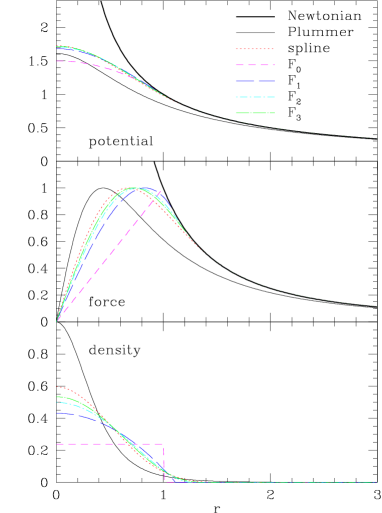
Figure 1: Potential, force, and density for Plummer and spline softening kernels as well as the Ferrers (1877) sphere kernels F_n. The softening lengths $\epsilon$ are scaled such that the maximal force equals unity.

The next best approximation to Newtonian gravity is the F₁ kernel (in the field of density estimation also known as “Epanechnikov” kernel). If its discontinuous second force derivative is a problem, one should use the F₂ kernel, while the spline kernel does not satisfy point 4 of the above list and also compares somewhat worse to Newtonian gravity than does the F₂ kernel (but see footnote 5).

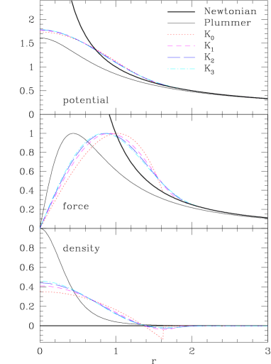
Figure 2: Like Figure 1, but for the kernels K_n and the Plummer kernel. Near their outer edge, these first kernels have negative density and forces that exceed those of Newtonian gravity. As a result, the under-estimation of the force field due to too small forces near the origin is largely compensated.

One may want to derive the kernel that minizes the asymptotic force error, i.e. $(b_{F}^{2}a_{0})$, subject to positivity and continuity. However, such an optimal kernel is likely to be only marginally better than, say, the F₁ kernel (which is optimal for one-dimensional density estimation, see Silverman 1986), at the price of having a significantly more complex functional form.

3.3.2 Kernels with bias compensation

In Appendix B, some simple kernels are derived which are low-order polynomials in $r^{2}$, yield $a_{0}=0$, and satisfy all points in the above list. These kernels, listed in Table 1 as K_n, have forces with continuous $n$th derivative. Figure 2 plots their potential, force, and density in comparison with Newtonian gravity and the Plummer kernel. While in the inner parts these kernels are harmonic, i.e. have vanishing forces like the kernels shown in Fig. 1, their forces exceed Newtonian gravity in the outer parts where their density is negative. This largly compensates the under-estimation of gravity in the inner parts and thus reduces the bias. As we shall see, these kernels prove to be superior for the purpose of force estimation, while for density estimation they are less useful because of their $\eta(r)$ not being non-negative.

4 adaptive softening lengths and      individual weights

To further improve the force estimation one may use locally adapted softening lengths and/or individual weights. Both techniques aim at enhancing the resolution in regions of high phase-space density by reducing $\epsilon$ or increasing the number density of bodies in such regions. Here, I will formally assess the effect of these possibilities on the force estimation.

4.1 Definitions

4.1.1 Individual weighting

The formalism behind this is to draw the initial positions $\{{\mn@boldsymbol{x}}_{i},{\mn@boldsymbol{v}}_{i}\}$ not from the DF $f({\mn@boldsymbol{x}},{\mn@boldsymbol{v}})$ modelled, but from a sampling DF $f_{\rm s}$, which is normalized to the same total mass $M$ as $f$. In this case, the bodies have individual weights

$$m_{i}=M\,N^{-1}\mu_{i},\quad\mu_{i}\equiv\mu({\mn@boldsymbol{x}}_{i},{\mn@boldsymbol{v}}_{i})$$ (21)

with the weight function

$$\mu({\mn@boldsymbol{x}},{\mn@boldsymbol{v}})\equiv f({\mn@boldsymbol{x}},{\mn@boldsymbol{v}})/f_{\rm s}({\mn@boldsymbol{x}},{\mn@boldsymbol{v}}),$$ (22)

i.e. lighter bodies are used to compensate for oversampling, corresponding to $f_{\rm s}$ being larger than $f$, and vice versa.

A potential problem with this method is an enhanced artificial heating of the population of low-mass bodies, e.g. modelling a stellar disk, by two-body interactions with high-mass bodies, e.g. modelling a dark halo. In order to overcome this problem, I propose below to use larger individual softening lengths for more massive particles.

4.1.2 Adaptive softening

For density estimation (see Silverman 1986), the usual procedure is to replace $\epsilon$ in equations (4) by $\epsilon\lambda_{i}$, resulting in the adaptive kernel estimators (with individual weights $m_{i}$):

(23)

So, $\epsilon$ no longer is a softening length, but the softening parameter that controls the overall degree of softening. The $\lambda_{i}$ are individual bandwidths, which are usually set to (Silverman 1986, p. 101) $\lambda_{i}\propto\hat{\rho}_{i}^{-\alpha}$ where $\hat{\rho}_{i}$ is an estimate for the density at ${\mn@boldsymbol{x}}_{i}$. The sensitivity parameter $\alpha$, a number satisfying $0\leq\alpha\leq 1$, determines how sensitive the local softening length is to variations in the density.

In the presence of individual weights, one may better use

$$\lambda_{i}=\mu_{i}^{1/2}\,\left(\hat{n}_{i}/\overline{n}\right)^{-\alpha},$$ (24)

where $\hat{n}_{i}$ are estimates of the local number density of bodies, while $\overline{n}$ is a normalization constant, hereafter the arithmetic mean of the $\hat{n}_{i}$. With this formula for the bandwidth, the maximal force in the neighbourhood of any body, ${\mn@boldsymbol{F}}_{\rm max}\propto m_{i}\lambda_{i}^{-2}$, is independent of $m_{i}$. For $\alpha=0$ and $\mu_{i}\equiv 1$ one obtains the standard fixed-kernel estimators (4).

The number of bodies within a softening volume is approximately

$$N_{\rm soft}\approx{4\pi\over 3}\,\epsilon^{3}\lambda_{i}^{3}n(x)\approx{4\pi\over 3}\,\epsilon^{3}\;\overline{n}^{3\alpha}\mu_{i}^{3/2}\;\hat{n}({\mn@boldsymbol{x}})^{1-3\alpha}.$$ (25)

Thus, the choice $\alpha=1/3$ results in $\mu_{i}^{-3/2}N_{\rm soft}$ being approximately constant over the entire system. In this case, one may, alternatively to equation (24), determine the local softening length such that the number of bodies within the softening volume is exactly proportional to $\mu_{i}^{3/2}$ (or constant if the bodies are equally weighted). In this case, the (fixed) number $\mu_{i}^{-3/2}N_{\rm soft}$ is the softening parameter.

In order to obtain the estimates $\hat{n}_{i}$ for the number densities, one may use the estimator

$$\hat{n}({\mn@boldsymbol{x}})={1\over\epsilon^{3}}\sum_{i=1}^{N}{1\over\lambda_{i}^{3}}\;\eta\left[{|{\mn@boldsymbol{x}}-{\mn@boldsymbol{x}}_{i}|\over\epsilon\lambda_{i}}\right].$$ (26)

with the bandwidths $\lambda_{i}$ from the previous time step.

If the method of individual weights is applied with $\alpha=0$, equation (24) implies that the bodies have individual, though non-adaptive, bandwidths. Note that this is by no means the only way incorporate $m_{i}$ into $\lambda_{i}$ – other ways may work as well, but here I only consider equation (24).

Hernquist & Katz (1991) dubbed this sort of adaptive softening the ‘scattering’ method. An alternative is the ‘gathering’ method, in which the softening length depends not on the gravity source (and its position ${\mn@boldsymbol{x}}_{i}$), but on the sink. A considerable disadvantage of both the scattering and the gathering method is the implied violation of momentum conservation. However, momentum conservation can easily be resurrected by using the same softening length $\epsilon_{ij}$ for the force of body $i$ on body $j$ and vice versa. Traditional choices are $\epsilon_{ij}^{2}=\epsilon^{2}(\lambda_{i}^{2}+\lambda_{j}^{2})$ (particularly useful in case of Plummer softening), $\epsilon_{ij}=\epsilon\,(\lambda_{i}+\lambda_{j})/2$ [Hernquist & Barnes 1990], or $\epsilon_{ij}=\epsilon\;{\rm min}(\lambda_{i},\lambda_{j})$. In a simulation of a galaxy group with each galaxy’s stellar component represented by a single spheroidal particle, which was considerably more massive than the halo bodies and therefore had larger bandwidth, Barnes (1985) used $\epsilon_{ij}=\epsilon\;{\rm max}(\lambda_{i},\lambda_{j})$, to avoid strong heating by individual halo body interactions.

4.2 Errors

4.2.1 The bias

The bias of the potential estimated using adaptive softening and individual weights is (see Appendices A.2 and A.3)

$${\rm bias}_{\mn@boldsymbol{x}}(\hat{\Phi})=a_{0}\,G\epsilon^{2}\rho({\mn@boldsymbol{x}})\,\overline{\mu}({\mn@boldsymbol{x}})\,\left[{n({\mn@boldsymbol{x}})\over\overline{n}}\right]^{-2\alpha}\;+\;{\cal O}(\epsilon^{4}),$$ (27)

where $\overline{\mu}\equiv\rho^{-1}\int\!{\rm d}^{3}\!\mn@boldsymbol{v}f\mu$ is the mass-weighted average of $\mu$ of all trajectories passing through ${\mn@boldsymbol{x}}$. This result is independent of the method used to assign $\epsilon_{ij}$ (it affects only the higher-order terms), while ${\rm bias}_{\mn@boldsymbol{x}}(\hat{{\mn@boldsymbol{F}}})={\mn@boldsymbol{\nabla}}{\rm bias}_{\mn@boldsymbol{x}}(\hat{\Phi})$.

Let us first consider $\mu\equiv 1$ (equal weighting). In this case, $n\propto\rho$ and therefore ${\rm bias}_{\mn@boldsymbol{x}}(\hat{{\mn@boldsymbol{F}}})\propto a_{0}\epsilon^{2}(1-2\alpha)\rho^{-2\alpha}{\mn@boldsymbol{\nabla}}\rho$. Compared to equation (LABEL:bias:force), the bias is reduced everywhere by the factor $(1-2\alpha)$ (for $\alpha=1/2$ we even have formally ${\rm bias}(\hat{{\mn@boldsymbol{F}}})={\cal O}(\epsilon^{4})$, but in this case the derivation of equation (27) becomes inconsistent, see Appendix A.2). Moreover, the factor $[\rho({\mn@boldsymbol{x}})/\overline{\rho}]^{-2\alpha}$ decreases the bias in high-density regions and increases it in low-density regions, such that the density-weighted ${\rm ISB}(\hat{{\mn@boldsymbol{F}}})$ is reduced.

If in addition $\mu\not\equiv 1$, the bias is further reduced. First $n({\mn@boldsymbol{x}})$ is a steeper function than $\rho({\mn@boldsymbol{x}})$ and hence $n^{-2\alpha}$ is shallower resulting in a smaller gradient (=${\rm bias}_{\mn@boldsymbol{x}}(\hat{{\mn@boldsymbol{F}}})$). Second, if the mean weight $\overline{\mu}$ is smaller in high-density regions, this produces a smaller gradient in the same way.

4.2.2 The variance

For the variance of the force, we obtain (see Appendices A.2 and A.3)

$$N{\rm var}_{\mn@boldsymbol{x}}(\hat{{\mn@boldsymbol{F}}})=b_{F}G^{2}M\epsilon^{-1}\rho({\mn@boldsymbol{x}})\,\overline{\mu^{1/2}}({\mn@boldsymbol{x}})\left[{n({\mn@boldsymbol{x}})\over\overline{n}}\right]^{\alpha}+{\cal O}(\epsilon^{0}).$$ (28)

Let us again first consider the case of equal weights. Then $n\propto\rho$, and ${\rm var}_{\mn@boldsymbol{x}}(\hat{{\mn@boldsymbol{F}}})\propto\rho^{1+\alpha}$, i.e. in contrast to the bias, the variance is enhanced in high density regions, because the softening length is reduced there. The corresponding increase in ${\rm IV}(\hat{{\mn@boldsymbol{F}}})$ is smaller than the decrease in ${\rm ISB}(\hat{{\mn@boldsymbol{F}}})$, because the density contrast $\rho/\overline{\rho}$ enters the integral for the evaluation of ${\rm IV}(\hat{{\mn@boldsymbol{F}}})$ only to the power $\alpha$, while in the evaluation of ${\rm ISB}(\hat{{\mn@boldsymbol{F}}})$ it enters to the power of $-4\alpha$. However, since at the optimal softening, $\mbox{${\rm IV}(\hat{{\mn@boldsymbol{F}}})$}=4\,\mbox{${\rm ISB}(\hat{{\mn@boldsymbol{F}}})$}$, the decrease in the ${\rm ISB}(\hat{{\mn@boldsymbol{F}}})$ must be more than four times the increase in the ${\rm IV}(\hat{{\mn@boldsymbol{F}}})$, in order to yield an overall improvement in the optimal ${\rm MISE}(\hat{{\mn@boldsymbol{F}}})$ (which occurs at larger $\epsilon$ than for the corresponding fixed-kernel estimate). Due to this effect, we do not necessarily expect a dramatic improvement of the force estimation from adaptive rather than fixed kernel estimators.

Consider next the situation for individual weights. We may replace $n$ by $\rho\overline{\mu^{-1}}$ to find that, compared to the equal-weight case, the variance is multiplied by $\overline{\mu^{1/2}\,}\overline{\mu^{-1}}^{\alpha}$. For $\mu_{i}$ not too far from unity, $\overline{\mu^{a}}\sim\overline{\mu}^{a}$ and the factor becomes $\sim\overline{\mu}^{1/2-\alpha}$. That is, for $\alpha\la 1/2$, the variance of the force is reduced in regions of smaller than average weights, decreasing the global measure ${\rm IV}(\hat{{\mn@boldsymbol{F}}})$.

Thus, when using individual weights in conjunction with adaptive softening, both variance and bias of the force are reduced in high-density regions and therefore also the mass-weighted averages ${\rm IV}(\hat{{\mn@boldsymbol{F}}})$ and ${\rm ISB}(\hat{{\mn@boldsymbol{F}}})$ as well as the overall force error ${\rm MISE}(\hat{{\mn@boldsymbol{F}}})$.

5 Numerical Experiments

So far, we have studied the properties of the softening purely analytically in the asymptotic limit of small $\epsilon$ and large $N$. In order to study the behaviour at finite $N$ and to assess the applicability of the asymptotic relations, we will now turn to numerical experiments. To this end, we compute the bias and the variance of the force at a hundred radii, $r_{k}$, equidistant in the enclosed mass, i.e. $M(<r_{k})=(k+{\textstyle{1\over 2}})/100$, and estimate the ${\rm ISB}(\hat{{\mn@boldsymbol{F}}})$ and ${\rm IV}(\hat{{\mn@boldsymbol{F}}})$ as averages over these points.

5.1 The targets

The comparisons will be made for two spherically symmetric models. The first is the Plummer (1911) sphere with density and potential

$$\rho(r)={3Mr_{s}^{2}\over 4\pi(r_{s}^{2}+r^{2})^{5/2}},\quad\Phi(r)=-{GM\over\sqrt{r_{s}^{2}+r^{2}}}.$$ (29)

(hereafter $G\equiv M\equiv r_{s}\equiv 1$), which has the advantage that most quantities in the above estimates can be evaluated analytically. The Plummer sphere has a harmonic core with central frequency $\omega=1$, i.e. $t_{\rm dyn}=2\pi$, in these units. I will also use the Hernquist (1990) model

$$\rho(r)={Mr_{s}\over 2\pi r(r_{s}+r)^{3}},\quad\Phi(r)=-{GM\over r_{s}+r}.$$ (30)

This model resembles the properties of galaxies better, since it has a central density cusp, where some of the asymptotic estimates made in Section 2 are not valid.

The Hernquist model has a central force ${\mn@boldsymbol{F}}\to-{\mn@boldsymbol{x}}/r$ as $r\equiv|{\mn@boldsymbol{x}}|\to 0$. Any softening yields a continuous force field and therefore inevitably gives $\langle\hat{{\mn@boldsymbol{F}}}\rangle=0$ in the centre, resulting in a 100% central force bias. Since this error is restricted to the softening volume where the density scales as $r^{-1}$, its contribution to the overall ${\rm ISB}(\hat{{\mn@boldsymbol{F}}})$ scales as $\epsilon^{2}$. Thus, because the ${\rm ISB}(\hat{{\mn@boldsymbol{F}}})$ for a non-cusped system scales as $\epsilon^{4}$, we expect the central bias to dominate the overall error for sufficiently small $\epsilon$, i.e. large $N$.

This is a generic problem of any cusped stellar system: the force field of a steep cusp cannot be resolved with any softening. Moreover, a cusp creates further problems for $N$-body simulations, since the dynamical time scale becomes arbitrary small as $r\to 0$. This means that one cannot even hope to properly model a cuspy stellar system with any $N$-body method, but must accept a small artificial core with size of the order of the softening length. Given this generic problem of all softening techniques, it makes sense to compare their performance only at $r>\epsilon$, i.e. ignore the problems at $r\to 0$. This is done automatically by our estimate of the ${\rm ISB}(\hat{{\mn@boldsymbol{F}}})$, since the smallest radius for which we compute the bias is non-zero (it contains 0.005 of the mass), i.e. larger than $\epsilon$ for small softening.

5.2 Fixed kernel estimates

5.2.1 Plummer sphere as target

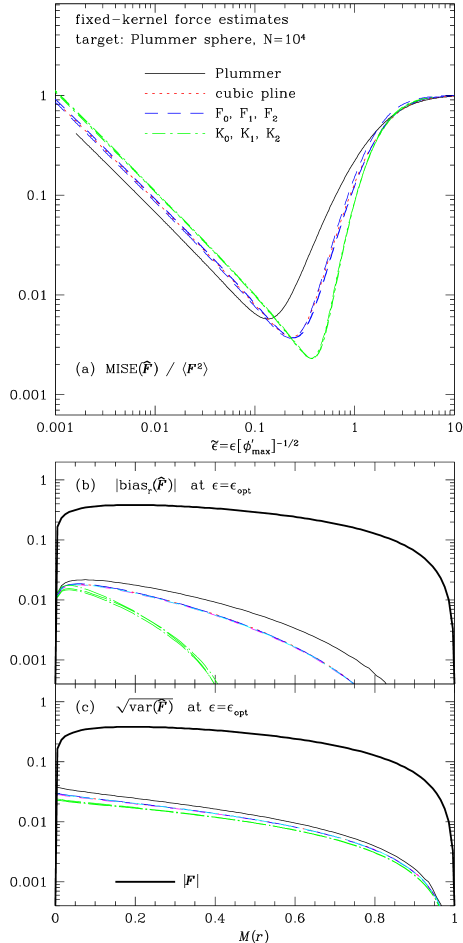
Figure 3: Fixed-kernel force estimate for most kernels of Table 1 applied to $N=10^{4}$ positions drawn from a Plummer sphere. In the top panel (a), the mean integrated squared force error, ${\rm MISE}(\hat{{\mn@boldsymbol{F}}})$, normalized by the averaged squared force of the Plummer sphere, is plotted vs. the scaled softening length $\tilde{\epsilon}$. The middle and bottom panels (b and c) give the radial run of the ${\rm bias}_{\mn@boldsymbol{x}}(\hat{{\mn@boldsymbol{F}}})$ and the dispersion, $[{\rm var}_{x}(\hat{{\mn@boldsymbol{F}}})]^{1/2}$, at the value of $\epsilon$ that minimizes the ${\rm MISE}(\hat{{\mn@boldsymbol{F}}})$. For comparison, the bold curve represents the true force in a Plummer sphere.

For most softening kernels of Table 1 (or Figures 1 and 2), Figure 3a plots the ${\rm MISE}(\hat{{\mn@boldsymbol{F}}})$, normalized by the averaged squared force

$$\langle{\mn@boldsymbol{F}}^{2}\rangle\equiv M^{-1}\int\!{\rm d}^{3}\!\mn@boldsymbol{x}\;\rho({\mn@boldsymbol{x}})\;{\mn@boldsymbol{F}}^{2}({\mn@boldsymbol{x}})$$ (31)

of the Plummer sphere, for $N=10^{4}$ bodies versus the scaled softening length

$$\tilde{\epsilon}=\epsilon\,\big{[}\phi^{\prime}(r_{{\rm max}\,F})\big{]}^{-1/2}.$$ (32)

The effect of this scaling is that the maximal force generated by a body of mass $m$ is $m/\tilde{\epsilon}^{2}$, independent of the kernel (the distance from the body at which this maximal force occurs is different for the different kernels, see Figs. 1 and 2).

In Figure 3a, the asymptotic behaviour at small and large softening lengths is immediately apparent. At small $\epsilon$, the integrated variance, ${\rm IV}(\hat{{\mn@boldsymbol{F}}})$, dominates the error budget, yielding a divergence as $\epsilon^{-1}$ for $\epsilon\to 0$. At fixed $\tilde{\epsilon}$, Plummer softening yields the smallest ${\rm IV}(\hat{{\mn@boldsymbol{F}}})$, which is related to its long-range softening.

At large $\epsilon$, the ${\rm MISE}(\hat{{\mn@boldsymbol{F}}})$ is dominated by the integrated squared bias, ${\rm ISB}(\hat{{\mn@boldsymbol{F}}})$, which increases steeply until $\tilde{\epsilon}\simeq 1$, beyond which it saturates at $\mbox{${\rm MISE}(\hat{{\mn@boldsymbol{F}}})$}=\langle{\mn@boldsymbol{F}}^{2}\rangle$, corresponding to a vanishing estimated force. As expected from our asymptotic results, the ${\rm ISB}(\hat{{\mn@boldsymbol{F}}})$ grows like $\epsilon^{4}$ for the compact kernels with non-negative density (cubic spline & F_n). For these kernels, the optimal scaled softening lengths and the resulting minimal ${\rm MISE}(\hat{{\mn@boldsymbol{F}}})$ are very similar. The latter is a consequence of the fact that the combination $E_{F}=b_{F}^{4}a_{0}^{2}$, through which the ${\rm MISE}_{\rm opt}(\hat{{\mn@boldsymbol{F}}})$ depends on the kernel, does not vary much between those kernels (see Table 1).

For Plummer softening, the ${\rm ISB}(\hat{{\mn@boldsymbol{F}}})$ is much larger (up to one order of magnitude) and grows approximately like $\epsilon^{3.3}$. As a result, the optimal softening length, $\tilde{\epsilon}_{\rm opt}$, is shorter (and hence the maximal force generated by any body larger) and the ${\rm IV}_{\rm opt}(\hat{{\mn@boldsymbol{F}}})$ as well as ${\rm MISE}_{\rm opt}(\hat{{\mn@boldsymbol{F}}})$ are larger than for compact kernels.

For the kernels K_n, which have partly-negative $\eta(r)$ and $a_{0}=0$, the ${\rm ISB}(\hat{{\mn@boldsymbol{F}}})$ is smaller than for the other kernels and grows like $\epsilon^{8}$ (for sufficiently small $\epsilon$). The ${\rm IV}(\hat{{\mn@boldsymbol{F}}})$ is only slightly larger than for the non-negative kernels, so that the minimal force error, ${\rm MISE}_{\rm opt}(\hat{{\mn@boldsymbol{F}}})$, is significantly smaller than for other kernels and occurs at larger $\tilde{\epsilon}$, i.e. the maximum force generated by a single body at optimal softening is smallest for these kernels.

Figures 3b and 3c show the radial run of the bias and dispersion, $[{\rm var}_{\mn@boldsymbol{x}}(\hat{{\mn@boldsymbol{F}}})]^{1/2}$, for the optimal softening, corresponding to the minima in Figure 3a. The lines for the four compact kernels with non-negative $\eta(r)$ almost overlay each other, as do the lines for the kernels K_n. This is exactly, what is expected from the asymptotic relations of Section 2, because of the similarity of the factors $E_{F}=b_{F}^{4}a_{0}^{2}$ and $b_{F}^{8}a_{2}^{2}$, respectively. In all cases, the dispersion is larger than the bias, in agreement with our expectations, based on the asymptotic relations, that $\mbox{${\rm IV}(\hat{{\mn@boldsymbol{F}}})$}=4\mbox{${\rm ISB}(\hat{{\mn@boldsymbol{F}}})$}$ (for compact kernels with $a_{0}\neq 0$). While in the inner parts of the Plummer sphere the bias contributes still significantly to the total error, in the outer parts the bias is neglible compared to the variance. This is true especially for the kernels K_n, which were designed to reduce the bias.

5.2.2 Hernquist model as target

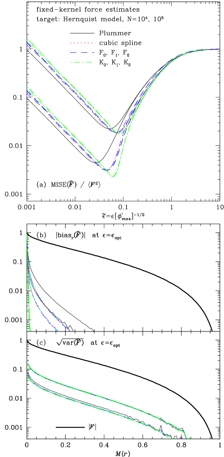
Figure 4: As Fig. 3 but for the Hernquist model as target with $N=10^{4}$ (upper curves) and $N=10^{5}$ (lower curves).

For $N=10^{4}$ and $10^{5}$, Figure 4 shows the results of fixed-kernel force estimation applied to a Hernquist model. Compared with the situation for the Plummer sphere (Fig. 3), the ${\rm IV}(\hat{{\mn@boldsymbol{F}}})$ (i.e. the MISE at small $\tilde{\epsilon}$) is only marginally larger at any $\tilde{\epsilon}$, as expected from the asymptotic relation: after normalisation by averaged squared force, the coefficient $B$ in equation (LABEL:B) is 20% larger than for the Plummer sphere. The ${\rm ISB}(\hat{{\mn@boldsymbol{F}}})$  on the other hand is significantly larger than for the Plummer sphere. This has the consequence that also the minimal ${\rm MISE}(\hat{{\mn@boldsymbol{F}}})$ is larger and occurs at smaller $\tilde{\epsilon}$ than for the Plummer sphere. In particular, at $N=10^{4}$, the relative rms force error $(\mbox{${\rm MISE}_{\rm opt}(\hat{{\mn@boldsymbol{F}}})$}/\langle\hat{{\mn@boldsymbol{F}}}\rangle)^{1/2}$ is as large as 14%, and still about 5% at $N=10^{5}$.

The differences in the ${\rm MISE}_{\rm opt}(\hat{{\mn@boldsymbol{F}}})$ between the various kernels are small at $N=10^{4}$ but become clearer at $N=10^{5}$: the improvement in increasing $N$ by an order of magnitude is significantly larger for the compact kernels, in particular K_n, than it is for Plummer softening.

As already discussed in Section 5.1, the central cusp of the Hernquist model causes a severe difficulty for any $N$-body method. The innermost radius for which we compute the bias and variance is $\approx 0.08$, and we thus expect the estimated ${\rm ISB}(\hat{{\mn@boldsymbol{F}}})$ to scale as $\epsilon^{2}$ for $\epsilon$ larger than this. The corresponding change in the slope is evident in Fig. 4a.

The radial runs of ${\rm bias}_{\mn@boldsymbol{x}}(\hat{{\mn@boldsymbol{F}}})$ and $[{\rm var}_{\mn@boldsymbol{x}}(\hat{{\mn@boldsymbol{F}}})]^{1/2}$ in Figs. 4b and c, respectively, are most interesting. In contrast to the situation for the Plummer sphere, the variance dominates at all body positions, except for the innermost few percent, especially for the kernels K_n, where the cusp results in a large bias.

5.3 Adaptive kernel estimates

Figures 4b and 4c nicely show the dilemma of fixed-kernels estimates: the large central ${\rm bias}_{\mn@boldsymbol{x}}(\hat{{\mn@boldsymbol{F}}})$ requires, in order to achieve the global balance between ${\rm ISB}(\hat{{\mn@boldsymbol{F}}})$ and ${\rm IV}(\hat{{\mn@boldsymbol{F}}})$, a small softening length, which in turn results in a large ${\rm var}_{\mn@boldsymbol{x}}(\hat{{\mn@boldsymbol{F}}})$ in the outer parts. It would be much better to balance bias and variance locally, in order to obtain an optimal mean square force error at every position ${\mn@boldsymbol{x}}$. By choosing the local softening length in proportion to $\rho^{-\alpha}$, the adaptive kernel estimates do not quite reach this goal, but certainly go a good way in the right direction.

There are many parameters which one may vary in adaptive kernel estimates: the kernels for the force and density estimators and their respective softening lengths as well as the sensitivity parameter $\alpha$. However, as we have seen in the fixed kernel estimates, the Plummer kernel is clearly inferior to the other kernels discussed, and there is not much difference between the various positive definite compact kernels or between the kernels K_n. Therefore, I will restrict the experiments to the F₁ and K₁ kernels for the force estimation, while the density is always estimated by the F₁ kernel. Since the variance of the estimated density (equation LABEL:var:density) increases much faster at small $\epsilon$ than that of the estimated force, the optimal softening parameter for density estimation is always larger than that for force estimation. Therefore, I use twice the softening scale for the evaluation of $\hat{\rho}({\mn@boldsymbol{x}}_{i})$ than in the force estimator.

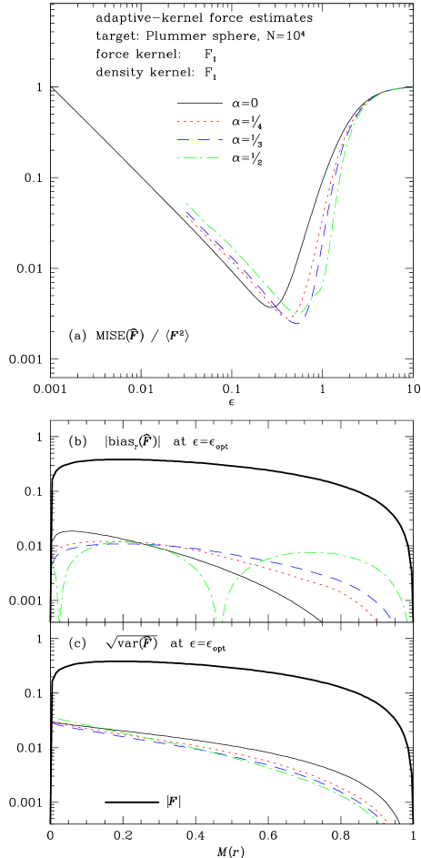
Figure 5: As Figure 3 but for an adaptive-kernel estimator based on the F₁ kernel. The softening scale of the density estimator has been set to twice that of the force estimator. Note that a sensitivity parameter of $\alpha=0$ corresponds to the fixed-kernel estimator of Fig. 3.

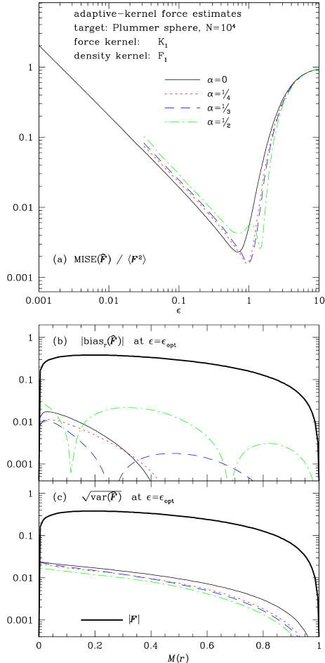
Figure 6: As Figure 5 but using the kernel K₁ in the force estimator

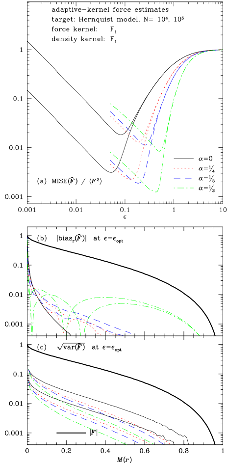
Figure 7: As Figure 4 but for an adaptive-kernel estimator based on the F₁ kernel. The softening scale of the density estimator has been set to twice that of the force estimator.

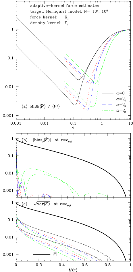
Figure 8: As Figure 7 but using the kernel K₁ in the force estimator

5.3.1 Plummer sphere as target

For various choices of the sensitivity parameter $\alpha$ (equation 24), Figures 5a and 6a show the run with $\epsilon$ of the ${\rm MISE}(\hat{{\mn@boldsymbol{F}}})$ obtained with the F₁ and K₁ kernels, respectively, from $N=10^{4}$ positions drawn from a Plummer sphere. The curves for $\alpha=0$ are identical to those of the corresponding kernel in Fig. 3. Adapting the local softening improves the accuracy of the force estimation: at $\alpha=1/3$ the ${\rm MISE}_{\rm opt}(\hat{{\mn@boldsymbol{F}}})$ has decreased by a factor of $\sim 1.6$, because the bias is substantially reduced, while the variance has been only slightly increased, in agreement with the expectations from theory in Section 4.2.

Out of the numbers tested for $\alpha$, the value $1/3$ results in the best estimate; the case $\alpha=1/2$ will be discussed seperately in Section 5.3.3.

It is very instructive to consider the radial run of bias and variance at $\epsilon=\epsilon_{\rm opt}$ in the lower panels of Figures 5 and 6. Compared to the fixed-kernel estimates ($\alpha=0$), the adaptive-kernel estimates have reduced variance, while the run of the bias is much shallower, exceeding that for $\alpha=0$ at large radii and running below it at small radii. Together this gives a better local balance between bias and variance and a local mean square force error, ${\rm MSE}_{\mn@boldsymbol{x}}(\hat{{\mn@boldsymbol{F}}})$ everywhere smaller than for the fixed-kernel estimators.

It should be noted that, in case of the compensating kernel K₁, already $\alpha=1/4$ results in a significant error reduction. For $\alpha=1/3$ and $\alpha=1/2$ (here also for F₁), the bias changes sign. In these cases, the bias is a rather complicated function of radius, the asymptotic form of which has not been derived above.

5.3.2 Hernquist model as target

Figures 7a and 8a plot the ${\rm MISE}(\hat{{\mn@boldsymbol{F}}})$ versus $\epsilon$ when applying the adaptive-kernel force estimator with, respectively, the F₁ and K₁ kernel to $N=10^{4}$ and $10^{5}$ positions drawn from the Hernquist model. As anticipated from the asymptotic relations in Section 4.2, the adaption reduces the ${\rm ISB}(\hat{{\mn@boldsymbol{F}}})$ (dominating the ${\rm MISE}(\hat{{\mn@boldsymbol{F}}})$at large $\epsilon$) substantially, much more than for the case of a Plummer sphere as target. However, the increase of the ${\rm IV}(\hat{{\mn@boldsymbol{F}}})$ is also quite large, so that the ${\rm MISE}_{\rm opt}(\hat{{\mn@boldsymbol{F}}})$ is reduced by about the same amount as for the Plummer target. A check with Figs. 7b&c and 8b&c shows that both ${\rm ISB}(\hat{{\mn@boldsymbol{F}}})$ and ${\rm IV}(\hat{{\mn@boldsymbol{F}}})$ are completely dominated by the large contributions from the innermost few per cent of the mass.

Interestingly, there is a difference between the kernels F₁ (with $a_{0}\neq 0$) and K₁ (with $a_{0}=0$): for the latter the adaption does not reduce the ${\rm MISE}_{\rm opt}(\hat{{\mn@boldsymbol{F}}})$ as much as for the F₁ kernel, and, as already found with the Plummer model as target (cf. Figure 6), the difference between $\alpha=1/4$ and $1/3$ is marginal.

5.3.3 What is the optimal $\alpha$?

Special attention must be given to the case $\alpha=1/2$, for which the asymptotic relation (27) breaks down. The behaviour both of the ${\rm MISE}(\hat{{\mn@boldsymbol{F}}})$ and of the ${\rm bias}_{\mn@boldsymbol{x}}(\hat{{\mn@boldsymbol{F}}})$ become strange at this choice of the sensitivity parameter. For example, in Fig. 7, $\alpha=1/2$ gives the smallest ${\rm MISE}_{\rm opt}(\hat{{\mn@boldsymbol{F}}})$, but the bias reaches $\sim 10\%$ in the outer regions of the model, where it usually is negligible. In other cases, $\alpha=1/2$ results in ${\rm MISE}(\hat{{\mn@boldsymbol{F}}})$ that behaves very odd as function of $\epsilon$, sometimes even with two minima (see Fig. 6a), and in most cases do not yield the smallest force error found.

The peculiar properties of $\alpha=1/2$ have been noticed in the context of density estimation a number of times (Scott 1992), in particular, that for large $N$ such estimates can be worse than fixed-kernel estimates – in agreement with Figure 6. This suggests that the behaviour of adaptive-kernel estimates with $\alpha=1/2$ is not well understood (even in the well-studied context of density estimation), and may thus be a topic for further investigations.

In the face of these results, the choice $\alpha=1/2$ cannot be recommended. However, a value of $1/3$ for the sensitivity parameter, corresponding to a roughly constant number of bodies within the local smoothing volume, seems to work well: it reduces the ${\rm MISE}_{\rm opt}(\hat{{\mn@boldsymbol{F}}})$ by a factor of about 1.6, the precise value depending on the circumstances (kernel & underlying model).

6 Discussion

6.1 Relevance for other than direct-summation codes

In our analysis, we have assumed that the forces are evaluated by direct summation, which is a rather CPU time intensive technique. Consequently, cheaper but approximate methods are favoured by most $N$-body engineers, with the exception of GRAPE [Ebisuzaki et al. 1993], which reaches a higher performance by wiring equation (3) into the hardware.

The force error arising from these approximate methods, some of which combine softening and approximation into one process, follows not necessarily the relation (15). Nonetheless, the ${\rm MISE}(\hat{{\mn@boldsymbol{F}}})$ is a function of $N$ because of ${\rm var}({\mn@boldsymbol{F}})\propto N^{-1}$. Of course, the force error also depends on the parameters of the method (including the softening length $\epsilon$). Hence, there exist optimal values for these parameters in the sense of minimizing the ${\rm MISE}(\hat{{\mn@boldsymbol{F}}})$ at given $N$.

This implies the necessity to change the parameters of the method when increasing $N$. However, this fact is often ignored by users of such techniques, who keep the parameters constant when increasing $N$ and then claim their method needs only ${\cal O}(N)$ or less operations for the force approximation. With such a practice, the force error will eventually be dominated by the bias, and increasing $N$ does not improve it at all. Moreover, the method becomes statistically inconsistent in the sense that in the limit $N\to\infty$ the estimated force does not converge to the true force. These last remarks apply in particular to the expansion and grid-based techniques discussed below.

6.1.1 The tree code

An important method is the Barnes & Hut (1986) tree code and its clones: the force is evaluated by direct summation for nearby bodies only, whereas distant bodies are grouped together and their gravity is computed via a low-order multipole expansion. This method reduces the computational costs to ${\cal O}(N\ln N)$ or even ${\cal O}(N)$ [Dehnen 2000].

The ignorance of the detailed structure of distant parts of the system introduces some additional errors and one objective of the $N$-body experimenter must be to keep these errors always smaller than those inherent to the force estimation (by softening). The results of Athanassoula et al. (1998) suggest that this condition is indeed satisfied for common-practice applications, which essentially implies that the results of this paper can be directly applied to the tree code.

6.1.2 Expansion techniques

Another method is based on an expansion of density and potential in a set of bi-orthogonal basis functions, ${\it\Phi}_{\mn@boldsymbol{n}}({\mn@boldsymbol{x}})$:

$$\hat{\Phi}({\mn@boldsymbol{x}})={\textstyle\sum}_{\mn@boldsymbol{n}}A_{\mn@boldsymbol{n}}{\it\Phi}_{\mn@boldsymbol{n}}({\mn@boldsymbol{x}}),\quad A_{\mn@boldsymbol{n}}={\textstyle\sum_{i}}m_{i}\,{\it\Phi}_{\mn@boldsymbol{n}}({\mn@boldsymbol{x}}_{i}).$$ (33)

where the second equality follows from the bi-orthogonality relation $4\pi\int\!{\rm d}^{3}\!\mn@boldsymbol{x}\,{\it\Phi}_{\mn@boldsymbol{m}}{\mn@boldsymbol{\nabla}}^{2}{\it\Phi}_{\mn@boldsymbol{n}}=\delta_{\mn@boldsymbol{n}\mn@boldsymbol{m}}$. The sum over $\mn@boldsymbol{n}$ in equation (33) includes terms up to some maximum $\mn@boldsymbol{n}_{\rm max}$ and contains ${\cal O}(n_{\rm max}^{3})$ terms in total.

This technique is important for special situations, in which the stellar system is closely matched, at all times, by the low-order basis functions. For example, when studying the stability of equilibrium systems of axial or polar symmetry, this is the method of choice [Earn & Sellwood 1995]. For less specialized investigations, the stellar system is not always well matched by the low-order basis functions, and the technique is essentially useless, because in this case $n_{\rm max}\propto N^{1/3}$ for optimal force estimation, resulting in computational costs that are ${\cal O}(n_{\rm max}^{3}\,N)={\cal O}(N^{2})$.

To see that $n_{\rm max}\propto N^{1/3}$ for the optimal force estimate, let us re-write equations (33) as weight-function estimate

$$\hat{\Phi}({\mn@boldsymbol{x}})={\textstyle\sum}_{i}m_{i}\,W({\mn@boldsymbol{x}}_{i},{\mn@boldsymbol{x}}),\;\;W({\mn@boldsymbol{x}},{\mn@boldsymbol{y}})\equiv{\textstyle\sum}_{\mn@boldsymbol{n}}{\it\Phi}_{\mn@boldsymbol{n}}({\mn@boldsymbol{x}}){\it\Phi}_{\mn@boldsymbol{n}}({\mn@boldsymbol{y}}).$$ (34)

The effective local softening length $\epsilon$ may be defined as the distance between zeros of the highest-order basis functions. While this varies with position and direction, it is obvious that $\epsilon\propto n^{-1}_{\rm max}$. The bias of the estimated force may be estimated in close analogy to the derivation in Appendix A.1.1. However, because $W({\mn@boldsymbol{x}},{\mn@boldsymbol{x}}+{\mn@boldsymbol{z}})$ is not reflection symmetric w.r.t. ${\mn@boldsymbol{z}}=0$, the bias is ${\cal O}(\epsilon)$ and not ${\cal O}(\epsilon^{2})$ as for kernel estimates. With ${\rm var}_{\mn@boldsymbol{x}}(\hat{{\mn@boldsymbol{F}}})\propto 1/N\epsilon$ we then find for the optimal softening $n_{\rm max}\propto N^{1/3}$ and $\mbox{${\rm MISE}_{\rm opt}(\hat{{\mn@boldsymbol{F}}})$}\propto N^{-2/3}$.

Thus, the main problem of the expansion technique is its large bias, arising from a mismatch, in all but special situations, between the stellar system and the set of basis functions. In order to overcome this fundamental problem, one must ensure that the low-order basis functions represent the stellar system fairly well [Hernquist & Ostriker 1992], for instance, by automatically adapting them to the stellar system modelled [Weinberg 1999].

6.1.3 Grid-based codes

Grid-based methods for the force evaluation are also quite common. In these methods, one estimates the density (via a kernel-estimator) on the nodes of a regular grid, solves for the potential and forces on these nodes by some grid method such as fast Fourier transforms, and finally interpolates the forces at the body positions. The density errors follow the relations of Section 2, but do not propagate trivially to the force estimate, because the grid method itself introduces further biases. Therefore, the detailled results of this paper may not be directly applied to grid-based methods, but the general remarks made at the beginning of this Section still hold.

6.2 Two-body relaxation

As already explained in the introduction, softening cannot much reduce the artificial two-body relaxation. The analytic results of Section 2 actually support this, which can be seen as follows.

Since relaxation is is driven by the graininess of gravity, it thus must be related to the variances of force and potential. In the limit $\epsilon\to 0$ of Newtonian gravity, the variations of the force actually diverge. However, in order to obtain the orbital changes one has to integrate the forces along the orbit, and this integral may no longer diverge. Actually, this integral must be related to the variation of the potential, since $\Phi=\int{\mn@boldsymbol{F}}\cdot\,{\rm d}{\mn@boldsymbol{x}}$. In contrast to the variance of the force, the variance of the potential is finite for Newtonian gravity, and it derives from the contributions not only of nearby stars, like the variance of the force, but from all stars. The same is true for the two-body relaxation, which suggests that it is related to the variance of the potential – though the situation must be more complex, since dynamical considerations (time variations) have to be taken into account.

From equation (LABEL:var:pot), it is clear that in order to reduce the integrated variance of the potential substantially, we need

$$\epsilon\simeq b_{\Phi}^{-1}\;{\int\!{\rm d}^{3}\!\mn@boldsymbol{x}\;\rho({\mn@boldsymbol{x}})\;{\rm var}_{\mn@boldsymbol{x}}^{0}(\Phi)\over\int\!{\rm d}^{3}\!\mn@boldsymbol{x}\;\rho^{2}({\mn@boldsymbol{x}})}.$$ (35)

For the Plummer sphere as underlying model and, say, the F₁ softening kernel, we get $\epsilon\simeq 1.1$ scale radii, implying that, unless the softening length is comparable to the size of the system itself, the variance of the potential cannot be significantly reduced by means of softening. This suggests that the usual small-scale softening does not much reduce the two-body relaxation in agreement with the arguments given in Section 1.1.1.

Table 2: Scaling with $N$ of the $\epsilon_{\rm opt}$ and ${\rm MISE}_{\rm opt}(\hat{{\mn@boldsymbol{F}}})$ for some softening methods applied to a Hernquist model

kernel	$\alpha$	${\rm MISE}_{\rm opt}(\hat{{\mn@boldsymbol{F}}})$		$\epsilon_{\rm opt}$
Plummer	0	0.000296$\,{\times}\,$	$N_{5}^{-0.77}$	0.017$\,{\times}\,$	$N_{5}^{-0.23}$
F1	0	0.000208$\,{\times}\,$	$N_{5}^{-4/5}$	0.051$\,{\times}\,$	$N_{5}^{-1/5}$
K1	0	0.000153$\,{\times}\,$	$N_{5}^{-8/9}$	0.115$\,{\times}\,$	$N_{5}^{-1/9}$
F1	$1/3$	0.000125$\,{\times}\,$	$N_{5}^{-4/5}$	0.186$\,{\times}\,$	$N_{5}^{-1/5}$
K1	$1/3$	0.000102$\,{\times}\,$	$N_{5}^{-8/9}$	0.309$\,{\times}\,$	$N_{5}^{-1/9}$

The ${\rm MISE}_{\rm opt}(\hat{{\mn@boldsymbol{F}}})$ was evaluated numerically for the Hernquist model sampled with $N=10^{5}$ points (see Section 5); $N_{5}\equiv N/10^{5}$. A sensitivity of $\alpha=0$ corresponds to a fixed-kernel estimate, i.e. constanst $\epsilon$.

6.3 What softening technique should one use?

Let us re-consider the scaling relations of the ${\rm MISE}(\hat{{\mn@boldsymbol{F}}})$ and $\epsilon_{\rm opt}$ with $N$. For various softening techniques, Table 2 lists them in the case of $N\sim 10^{5}$ and the Hernquist model as target. The numbers given in this table are based on the numerical results of Section 5 and the scaling relations of Section 3 also summarized in Table 3 below.

6.3.1 The softening method

We first concentrate on simple fixed-kernel estimators. When the standard Plummer kernel is replaced by a compact kernel (e.g. F₁) or a compensating kernel (e.g. K₁), the ${\rm MISE}_{\rm opt}(\hat{{\mn@boldsymbol{F}}})$ drops by a factor of $\sim 1.5$ and $\sim 2$, respectively. Note that such a change requires no overhead at all. Even codes using the cubic spline kernel of Monaghan & Lattanzio (1985) might benefit from employing the F₁ or K₁ kernel instead, since their computation involves less operations and the latter gives more accurate forces.

Another improvement by a factor of $\sim 1.5$ can be achieved by adapting the softening lengths locally in such a way that the number $N_{\rm soft}$ of bodies in the softening volume is roughly constant (but dependent on $N$). This result for the Hernquist model as target applies to a lesser degree to stellar system with a smaller dynamic range, e.g. with a density core like the Plummer model.

6.3.2 How to choose $\epsilon$?

There are actually two questions behind this one, both of vital importance to the subject, neither of which has been addressed so far. First, how to find the value for $\epsilon$ that minimizes the ${\rm MISE}(\hat{{\mn@boldsymbol{F}}})$ if the true underlying force field is unknown (e.g. during a $N$-body simulation) and, second, is $\epsilon_{\rm opt}$ derived in this way really the best choice?

Merritt (1996) presumed that a time-intensive boot-strap algorithm would be needed to find $\epsilon_{\rm opt}$ if ${\mn@boldsymbol{F}}({\mn@boldsymbol{x}})$ were unknown. However, if $N$ is large enough for the asymptotic relations of Section 2 to hold, one may exploit these in order to find $\epsilon_{\rm opt}$ with an overhead comparable to one full force computation for all bodies. The details of this method and some performance tests will be given in a follow-up paper.

Table 3: Asymptotic scaling relations with $\epsilon$ and $N$

kernel	${\rm bias}(\hat{{\mn@boldsymbol{F}}})$	$\epsilon_{\rm opt}$	${\rm MISE}_{\rm opt}(\hat{{\mn@boldsymbol{F}}})$
Plummer	$\propto\epsilon^{1.67}$	$\propto N^{-0.23}$	$\propto N^{-0.77}$
compact	$\propto\epsilon^{2}$	$\propto N^{-1/5}$	$\propto N^{-4/5}$
compensating	$\propto\epsilon^{4}$	$\propto N^{-1/9}$	$\propto N^{-8/9}$

Note that ${\rm var}(\hat{{\mn@boldsymbol{F}}})$ always scales as $\epsilon^{-1}N^{-1}$, so the scaling of ${\rm bias}(\hat{{\mn@boldsymbol{F}}})$ makes all the difference.

The second question is less technical and more difficult to answer. The error of the force comes in two parts, bias and variance. In the time mapping of the DF, these will give rise to different artificial effects. The variance results in enhanced relaxation, while the bias modifies the stellar dynamics; moreover there might be some interplay between the two. It is not clear and non-trivial to say, what the consequences of these modifications are and how they scale with simulation time. It is likely that the optimal $\epsilon$ depends both on the stellar system modelled and on the specific goal of the simulation. If, for instance, the stability of some equilibrium configuration is to be investigated, it is essential to modify gravity as little as possible, i.e. use small $\epsilon$ (and a compensating kernel). On the other hand, when more violent dynamics is investigated (e.g. mergers) one might want to suppress small-scale noise. Obviously, these are important issues which deserve further investigations.

6.4 The optimal collisionless $\mn@boldsymbol{N}$-body code

Merritt (1996) proposed to call a Poisson solver optimal if it results in the smallest ${\rm MISE}(\hat{{\mn@boldsymbol{F}}})$ for given $N$. With this definition, all non-direct methods are sub-optimal (since, in addition to the softening, they invoke approximations, which introduce additional errors), and yet such methods are generally preferred. Therefore, one may better define: The optimal collisionless $N$-body code achieves, for given computer resources (CPU time and memory), the most faithful time-mapping of those properties of the DF that are essential for the purpose of the particular simulation. Note that in this definition, the number $N$ of bodies does not occur, $N$ is just a parameter of the code, as is the softening length. This means in particular, that contrary to widespread practice, the number $N$ alone is not a sufficient criterion for the quality of a $N$-body simulation.

What is the optimal Poisson solver for general-purpose collisionless $N$-body codes? From the discussion in Section 6.1, it is clear that expansion techniques are not suitable for a general applicable $N$-body code – unless, perhaps, Weinberg’s (1999) automatic adaption method is continuously applied. Obviously, the optimal Poisson solver must be adaptive in space and time. This condition clearly favours the tree code, which naturally is fully adaptive, while for grid-based solvers a considerable effort is needed to make them fully adaptive.

From the results of this paper, it appears to be obvious that the optimal softening method uses adaptive softening lengths and a compact, or even compensating, kernel. A fixed softening length may be appropriate in the case of a stellar system with a small dynamic range, i.e. with a constant-density core.

6.5 On the resolution of a $\mn@boldsymbol{N}$-body simulation

In discussing $N$-body simulations, it is important to know their resolution scale, i.e. the smallest scale on which a simulation is “believable”. Lacking a more precise definition, one often simply uses the softening length $\epsilon$ for the resolution scale. With the asymptotic relations in Table 3, this yields the absurd result that users of Plummer softening can improve the resolution of their simulations faster with increasing $N$ than users of compact or compensating kernels, which we have shown to be superior to Plummer softening. How can this be?

The problem is that linearly relating $\epsilon$ with resolution scale is incorrect. The softening length $\epsilon$ is a mere parameter without any physical meaning. A force resolution length may be properly defined as the scale over which the maximum change in the true force equals the (local) error of the estimated force:

$$s_{\rm res}({\mn@boldsymbol{x}})\approx{\sqrt{{\rm MSE}_{\mn@boldsymbol{x}}(\hat{{\mn@boldsymbol{F}}})}\over\|{\mn@boldsymbol{\nabla}}\otimes{\mn@boldsymbol{F}}({\mn@boldsymbol{x}})\|}.$$ (36)

With the results of Section 2, we find that, for optimally chosen $\epsilon$, the decrease of $s_{\rm res}$ with increasing $N$ is slowest for Plummer softening and fastest for softening with compensating kernels. In particular, the relation between $\epsilon$ and $s_{\rm res}$ is non-linear.

Note, however, that $s_{\rm res}$ defined above is a mere measure for the resolution of the force, and not of the believability of the simulation. Since gravity is a long-range force, local errors in the DF, introduced on scales of $s_{\rm res}$, may well propagate to larger scales.

7 Summary and conclusion

In collisionless $N$-body simulations, the bodies are the numerical representation of the continuous one-particle DF. Because $N$ is much smaller than in the stellar system being modelled, this representation is always incomplete, i.e. noisy. In order to estimate, at each time step, the continuous force field due to the DF, one has to moderate this noise. This exactly is the purpose of force softening in collisionless $N$-body codes. However, while reducing the noise in the $N$-body forces, the softening modifies the laws of gravity: the force vanishes at vanishing inter-body separation $r\to 0$. This generates a bias, a systematic offset between the estimated and true forces. Both, the noise and the bias, contribute to the mean square error of the estimated force field. While the noise decreases with the softening length $\epsilon$, the bias increases, and the optimal softening represents a compromise between these two [Merritt 1996].

In the limit of $\epsilon$ being small compared to any physical scale of the stellar system, a requirement that is desirably satisfied in any $N$-body simulation, analytic expressions for the noise-generated variance of the force and for the bias have been derived. While the relations (LABEL:bias) for the bias have already been given in the literature (e.g. Hernquist & Katz 1989), those for the variance of the estimated potential and force (equation 11) seem to be hitherto unknown. One of the most important results is that the variance of the force is a local quantity diverging in the limit $\epsilon\to 0$, very much like the variance of the density, while the variance of the potential depends on a global measure and reaches a finite value for $\epsilon=0$. Presumably, this is related to the fact, see Section 6.2 and Theis (1998), that the two-body relaxation is not substantially reduced by force softening.

In these asymptotic relations, the effects of the softening length, the softening kernel, the number $N$ of bodies, and of the underlying stellar system nicely separate, allowing simple and, in the important case of large $N$, accurate estimates for the behaviour of the mean integrated squared force error, ${\rm MISE}(\hat{{\mn@boldsymbol{F}}})$. For the various types of softening kernels, Table 3 gives the asymptotic relations for the optimal softening length and force errors (the relations given for Plummer softening are based on numerical experiments only). The strongest possible dependence of the MISE on $N$ is $N^{-1}$ as pertains, e.g., to parametric estimators. Note that the compensating kernels come very close to this limit. The main results of this investigation are:

• Compact softening kernels, i.e. those with finite density support, are superior to the standard Plummer softening. This improvement is ever larger for increasing $N$.

• Special softening kernels are derived, for which the force errors are even smaller. These kernels compensate the small forces at $r\to 0$ by forces larger than Newtonian at $r\sim\epsilon$.

• For inhomogeneous stellar systems, such as galaxies, adaptive softening lengths allow a further substantial reduction of the force errors.

All these numbers are based on the Hernquist model, which gives a fair representation of a typical galaxy, as underlying stellar system, resulting in a rms force error of $\sim 0.01=0.04$ of the rms force of this model. For smaller errors to be achieved, the advantage of using compensating kernels and adaptive softening lengths will become even larger.

For this error of 4%, particle numbers $N\sim 10^{5}$ are necessary, and roughly 20 times as many to reduce the error to 1%. It is not clear, what these errors imply in terms of the reliability of the time evolution of a corresponding $N$-body simulation. This is a very important question to answer, in order to better understand the results of $N$-body simulations and assess their reliability. For example, current $N$-body simulations of large-scale structure formation employ only about $10^{3-4}$ bodies per halo, which come out to have a profile similar to a Hernquist model, i.e. the rms force error is $10\%$ to $25\%$, even if $\epsilon$ was chosen optimally, which it very likely was not.

Appendix A Asymptotic Relations for Bias and Variance

A.1 Fixed-kernel estimates with equal weights

A.1.1 The bias

In calculating the expectation value, we may replace the sum over points by an integral weighted with the density $\rho$. Thus

$$\big{\langle}\hat{\Phi}({\mn@boldsymbol{x}})\big{\rangle}=-{G\over\epsilon}\int\!{\rm d}^{3}\!\mn@boldsymbol{y}\;\rho({\mn@boldsymbol{y}})\;\phi\left[{|{\mn@boldsymbol{x}}-{\mn@boldsymbol{y}}|\over\epsilon}\right].$$ (37)

We proceed by writing

$${1\over\epsilon}\,\phi\left({r\over\epsilon}\right)={1\over r}-{1\over\epsilon}\left[{\epsilon\over r}-\phi\left({r\over\epsilon}\right)\right].$$ (38)

Inserting this into equation (37) and substituting ${\mn@boldsymbol{y}}={\mn@boldsymbol{x}}-\epsilon{\mn@boldsymbol{z}}$, we find

$$\big{\langle}\hat{\Phi}({\mn@boldsymbol{x}})\big{\rangle}=\Phi({\mn@boldsymbol{x}})+G\,\epsilon^{2}\int\!{\rm d}^{3}\!\mn@boldsymbol{z}\;\left[{1\over|{\mn@boldsymbol{z}}|}-\phi(|{\mn@boldsymbol{z}}|)\right]\;\rho({\mn@boldsymbol{x}}-\epsilon{\mn@boldsymbol{z}}).$$ (39)

When replacing $\rho({\mn@boldsymbol{x}}-\epsilon{\mn@boldsymbol{z}})$ by its Taylor expansion about ${\mn@boldsymbol{x}}$,

$$\rho({\mn@boldsymbol{x}}-\epsilon{\mn@boldsymbol{z}})=\sum_{k\geq 0}{(-\epsilon)^{k}\over k!}({\mn@boldsymbol{z}}{\mn@boldsymbol{\nabla}})^{k}\rho({\mn@boldsymbol{x}}),$$ (40)

we see that, by virtue of the symmetry of the kernel, the integrals over all odd orders in $\epsilon$ vanish identically and one obtains

$${\rm bias}_{\mn@boldsymbol{x}}(\hat{\Phi})=a_{0}\,\epsilon^{2}G\,\rho({\mn@boldsymbol{x}})+a_{2}\,\epsilon^{4}G\,\Delta\rho({\mn@boldsymbol{x}})+{\cal O}(\epsilon^{6})$$ (41)

where

$$a_{k}={4\pi\over(k+1)!}\int_{0}^{\infty}{\rm d}r\;r^{k+2}\left[{1\over r}-\phi(r)\right]={4\pi\over(k+1)!\,(k+3)}\int_{0}^{\infty}{\rm d}r\;r^{k+3}\left[{1\over r^{2}}+\phi^{\prime}(r)\right]={(4\pi)^{2}\over(k+3)!}\int_{0}^{\infty}{\rm d}r\;r^{k+4}\eta(r).$$ (42)

A similar estimate can be made for the bias of the force and density estimators in equations (LABEL:soft:force) and (LABEL:soft:density), but it is actually simpler to relate the biases directly using Poisson’s equation. Note, that the integrals over $\!{\rm d}^{3}\!\mn@boldsymbol{z}$ in equation (39) may not converge if the kernel does not approach its asymptotic shape $\phi\to 1/r$ fast enough at large radii. To be more precise, if the density kernel $\eta$ falls off as $r^{-5}$ or less steeply, then the biases grow faster than quadratically with small $\epsilon$.

Furthermore, if the Taylor expansion in equation (40) does not converge, the above estimate is incorrect, too, usually over-estimating the true bias. To see this, consider a spherical cusp in the density at ${\mn@boldsymbol{y}}=0$, i.e. $\rho=\rho_{0}y^{-\gamma}$ (with $\gamma<2$) at small $y$. Inserting this instead of the Taylor expansion into equation (39), we find for $x\ll\epsilon$

(43)

Here, the integrals extend only formally to infinity: for a sensible kernel, the term in brackets vanishes outside some small radius. Thus, for cusps shallower than $\gamma=1$, the bias in the force is still finite; for steeper cusps, the correct force actually diverges, which of course cannot be reproduced by the softening, resulting in a diverging force bias.

A.1.2 The variance

Assuming the positions ${\mn@boldsymbol{x}}_{i}$ are independent, the variance of some quantity is equal to $N^{-1}$ times the variance of the contribution of one point. Moreover, the central-limit theorem tells us that the estimates follow essentially a normal distribution.

The variance of the estimated potential.

With ${\mn@boldsymbol{r}}_{i}={\mn@boldsymbol{x}}_{i}-{\mn@boldsymbol{x}}$, the contribution of one point is $\phi_{i}({\mn@boldsymbol{x}})\equiv-GM\,\epsilon^{-1}\phi(|{\mn@boldsymbol{r}}_{i}|/\epsilon)$. Thus, from equation (LABEL:var) we have

$$N{\rm var}_{\mn@boldsymbol{x}}(\hat{\Phi})=\big{\langle}\phi_{i}^{2}({\mn@boldsymbol{x}})\big{\rangle}-\big{[}\Phi({\mn@boldsymbol{x}})+{\rm bias}_{\mn@boldsymbol{x}}(\hat{\Phi})\big{]}^{2}.$$ (44)

We may evaluate $\langle\phi\rangle_{i}^{2}$ as an average weighted with the density $\rho$:

$$\big{\langle}\phi_{i}^{2}({\mn@boldsymbol{x}})\big{\rangle}={G^{2}M\over\epsilon^{2}}\int\!{\rm d}^{3}\!\mn@boldsymbol{y}\;\rho({\mn@boldsymbol{y}})\,\phi^{2}\left({|{\mn@boldsymbol{x}}-{\mn@boldsymbol{y}}|\over\epsilon}\right).$$ (45)

We proceed by writing

$${1\over\epsilon^{2}}\;\phi^{2}\Big{(}{r\over\epsilon}\Big{)}={1\over r^{2}}+{1\over\epsilon^{2}}\left[\phi^{2}\Big{(}{r\over\epsilon}\Big{)}-{\epsilon^{2}\over r^{2}}\right]$$ (46)

to finally obtain

$$\big{\langle}\phi^{2}_{i}({\mn@boldsymbol{x}})\big{\rangle}=G^{2}M\left\{\left[\int\!{\rm d}^{3}\!\mn@boldsymbol{y}\;{\rho({\mn@boldsymbol{y}})\over({\mn@boldsymbol{x}}-{\mn@boldsymbol{y}})^{2}}\right]-\epsilon\,b_{\Phi}\,\rho({\mn@boldsymbol{x}})+{\cal O}(\epsilon^{2})\right\}$$ (47)

with $b_{\Phi}=4\pi\,\int_{0}^{\infty}{\rm d}r\,[1-r^{2}\phi^{2}(r)]$.

The variance of the estimated force.

The contribution from one body is $\mn@boldsymbol{f}_{i}={\mn@boldsymbol{r}}_{i}/|{\mn@boldsymbol{r}}_{i}|\,G\,M\,\epsilon^{-2}\phi^{\prime}(|{\mn@boldsymbol{r}}_{i}|/\epsilon)$, and in analogy to equation (45), we have

$$\big{\langle}\mn@boldsymbol{f}_{i}\otimes\mn@boldsymbol{f}_{i}\big{\rangle}={G^{2}M\over\epsilon^{4}}\int\!{\rm d}^{3}\!\mn@boldsymbol{y}\;\rho({\mn@boldsymbol{y}})\;\phi^{\prime 2}\left({|{\mn@boldsymbol{x}}-{\mn@boldsymbol{y}}|\over\epsilon}\right)\;{({\mn@boldsymbol{x}}-{\mn@boldsymbol{y}})\otimes({\mn@boldsymbol{x}}-{\mn@boldsymbol{y}})\over({\mn@boldsymbol{x}}-{\mn@boldsymbol{y}})^{2}}.$$ (48)

Substituting ${\mn@boldsymbol{y}}={\mn@boldsymbol{x}}-\epsilon{\mn@boldsymbol{z}}$ and Taylor expanding $\rho$, we find for the variance

$${\rm var}_{\mn@boldsymbol{x}}(\hat{{\mn@boldsymbol{F}}})=G^{2}\,\epsilon^{-1}\,M\,N^{-1}\,b_{F}\,\rho({\mn@boldsymbol{x}})\,{\textstyle{1\over 3}}\mn@boldsymbol{\sf I}\;+\;{\cal O}(\epsilon^{0}),$$ (49)

where $\mn@boldsymbol{\sf I}$ denotes the unit matrix, while $b_{F}=4\pi\,\int_{0}^{\infty}{\rm d}r\,r^{2}\phi^{\prime 2}(r)$.

The variance of the estimated density.

The contribution from one body is $\rho_{i}=M\,\epsilon^{-3}\eta(|{\mn@boldsymbol{r}}_{i}|/\epsilon)$, and

$$\big{\langle}\rho_{i}^{2}\big{\rangle}={M^{2}\over\epsilon^{6}}\int\!{\rm d}^{3}\!\mn@boldsymbol{y}\;\rho({\mn@boldsymbol{y}})\;\eta^{2}\left({|{\mn@boldsymbol{x}}-{\mn@boldsymbol{y}}|\over\epsilon}\right)=M^{2}\epsilon^{-3}\,b_{\rho}\,\rho({\mn@boldsymbol{x}})+{\cal O}(\epsilon^{-1})$$ (50)

with $b_{\rho}=\int_{0}^{\infty}{\rm d}r\,r^{2}\eta^{2}(r)$.

A.2 Adaptive softening with equal weights

In analogy to equation (39), we get for the expectation value of the estimated potential

$$\big{\langle}\hat{\Phi}({\mn@boldsymbol{x}})\big{\rangle}=\Phi({\mn@boldsymbol{x}})+G\epsilon^{2}\int\!{\rm d}^{3}\!\mn@boldsymbol{z}\;{\rho({\mn@boldsymbol{x}}-\epsilon{\mn@boldsymbol{z}})\over\lambda}\,\left[{1\over r}-\phi(r)\right]_{r=|{\mn@boldsymbol{z}}|/\lambda}.$$ (51)

For equal weights, equation (24) reduces to $\lambda=[\hat{\rho}({\mn@boldsymbol{x}}-\epsilon{\mn@boldsymbol{z}})/\overline{\rho}]^{-\alpha}$. In order to estimate the asymptotic behaviour at small $\epsilon$, we may replace $\hat{\rho}$ in this relation by $\rho$. For kernels with $a_{0}\neq 0$, the error made by this assumption is ${\cal O}(\epsilon^{2})$ and hence the resulting error in the bias of the potential is a factor $\epsilon^{2}$ smaller than the leading term. We thus get

$${\rm bias}_{\mn@boldsymbol{x}}(\hat{\Phi})=a_{0}\,G\,\epsilon^{2}\,\overline{\rho}^{2\alpha}\rho({\mn@boldsymbol{x}})^{1-2\alpha}+{\cal O}(\epsilon^{4}).$$ (52)

which for $\alpha=0$ reduces to the result for the fixed-kernel estimate.

For $\alpha=1/2$, the quadratic term in ${\rm bias}(\hat{\Phi})$ is constant and the biases of force and density are formally only ${\cal O}(\epsilon^{4})$. However, this was not anticipated in the approximation made above, where $\hat{\rho}$ in the definition of $\lambda$ was replaced by $\rho$. Thus, for this special case, the estimation might be incorrect.

Because the variances are dominated by the lowest order in $\epsilon$, we may use the above relations for the fixed-kernel estimates with $\epsilon$ replaced with $\epsilon[\rho({\mn@boldsymbol{x}})/\overline{\rho}]^{-\alpha}$.

A.3 Softening with individual weights

In this case, the softening lengths $\epsilon\lambda_{i}$ depend on the full 6D phase-space coordinates, and we must replace the density-weighted averaging over configuration space by a sampling-distribution-function-weighted averaging over phase space.

A.3.1 The bias

With equation (38) we obtain

$${\rm bias}_{\mn@boldsymbol{x}}(\hat{\Phi})={G\over\epsilon}\int\!{\rm d}^{3}\!\mn@boldsymbol{y}\int\!{\rm d}^{3}\!\mn@boldsymbol{v}\;f_{\rm s}({\mn@boldsymbol{y}},{\mn@boldsymbol{v}})\;{\mu({\mn@boldsymbol{y}},{\mn@boldsymbol{v}})\over\lambda({\mn@boldsymbol{y}},{\mn@boldsymbol{v}})}\;\left[{1\over r}-\phi(r)\right]_{r=|{\mn@boldsymbol{x}}-{\mn@boldsymbol{y}}|/\epsilon\lambda({\mn@boldsymbol{y}},{\mn@boldsymbol{v}})}$$ (53)

with

$$\lambda({\mn@boldsymbol{y}},{\mn@boldsymbol{v}})=\mu({\mn@boldsymbol{y}},{\mn@boldsymbol{v}})^{1/2}\;[\hat{n}({\mn@boldsymbol{y}})/\overline{n}]^{-\alpha},$$ (54)

where $\mu({\mn@boldsymbol{y}},{\mn@boldsymbol{v}})$ is given in equation (22). In order to proceed, we first replace $\hat{n}$ by $n$ in the definition of $\lambda$ in analogy to the equal-weight case, and second substitute ${\mn@boldsymbol{y}}={\mn@boldsymbol{x}}-\epsilon\lambda{\mn@boldsymbol{z}}$ with $|{\rm d}{\mn@boldsymbol{y}}/{\rm d}{\mn@boldsymbol{z}}|=\epsilon^{3}\lambda^{3}({\mn@boldsymbol{x}},{\mn@boldsymbol{v}})+{\cal O}(\epsilon^{4}z)+{\cal O}(\epsilon^{5}z^{2})$. We then finally get

$${\rm bias}_{\mn@boldsymbol{x}}(\hat{\Phi})=a_{0}\,G\epsilon^{2}\,\rho({\mn@boldsymbol{x}})\,\overline{\mu}({\mn@boldsymbol{x}})\,[n({\mn@boldsymbol{x}})/\overline{n}]^{-2\alpha}\;+\;{\cal O}(\epsilon^{4}),$$ (55)

where $\overline{\mu}=\overline{\mu^{1}}$ with $\overline{\mu^{a}}\equiv\rho^{-1}\int\!{\rm d}^{3}\!\mn@boldsymbol{v}f\mu^{a}$ the mass-weighted average of $\mu^{a}$ of all trajectories passing through ${\mn@boldsymbol{x}}$.

A.3.2 The variance

For the force variance, we have instead of equation (48)

$$\big{\langle}\mn@boldsymbol{f}_{i}\otimes\mn@boldsymbol{f}_{i}\big{\rangle}={G^{2}M\over\epsilon^{4}}\int\!{\rm d}^{3}\!\mn@boldsymbol{y}\int\!{\rm d}^{3}\!\mn@boldsymbol{v}\;f_{\rm s}({\mn@boldsymbol{y}},{\mn@boldsymbol{v}})\,{\mu({\mn@boldsymbol{y}},{\mn@boldsymbol{v}})^{2}\over\lambda({\mn@boldsymbol{y}},{\mn@boldsymbol{v}})^{4}}\;\phi^{\prime 2}\left({|{\mn@boldsymbol{x}}-{\mn@boldsymbol{y}}|\over\epsilon}\right)\;{({\mn@boldsymbol{x}}-{\mn@boldsymbol{y}})\otimes({\mn@boldsymbol{x}}-{\mn@boldsymbol{y}})\over({\mn@boldsymbol{x}}-{\mn@boldsymbol{y}})^{2}}.$$ (56)

When substituting ${\mn@boldsymbol{y}}={\mn@boldsymbol{x}}-\epsilon\lambda{\mn@boldsymbol{z}}$ and using equation (54), we get for the force variance to lowest order in $\epsilon$

$${\rm var}_{\mn@boldsymbol{x}}(\hat{{\mn@boldsymbol{F}}})=G^{2}\,\epsilon^{-1}\,M\,N^{-1}\,b_{F}\,\rho({\mn@boldsymbol{x}})\;\overline{\mu^{1/2}}({\mn@boldsymbol{x}})\;[n({\mn@boldsymbol{x}})/\overline{n}]^{\alpha}\;+{\cal O}(\epsilon^{0}).$$ (57)

Note that for $\alpha=0$ these relations do not reduce to those given for fixed-kernel estimates, because, with our definition of $\lambda_{i}$ (equation 24), individual weights also result in individual bandwidths.

Appendix B Investigations for better kernels

We want to design a spherical kernel $\phi(r)$ that corresponds to a compact density $\eta(r)$ and satisfies all conditions listed in Section 3.3. Let us therefore assume that $\eta(r)=0$ and $\phi(r)=r^{-1}$ for $r>1$. Moreover, continuity of $\phi$ and the normalization of $\eta$ give us the constraints

$$\phi^{\prime}(0)=0,\qquad\phi(1)=1,\qquad\phi^{\prime}(1)=-1.$$ (58)

Let us now make an ansatz for $\phi$ that, in order to satisfy point 4 of the list in Section 3.3, involves only powers of $r^{2}$ for $r<1$:

$$\phi=\sum_{k\geq 0}\,C_{k}\,(1-r^{2})^{k}\quad{\rm for}\;r\leq 1\qquad{\rm and}\qquad\phi=r^{-1}\quad{\rm otherwise}.$$ (59)

The constraints (58) require $C_{0}=1$ and $C_{1}={\textstyle{1\over 2}}$, but do not require anything for the higher-order coefficients. When these are all set to zero, one obtains the homogeneous-sphere kernel.

B.1 Ferrers sphere kernels

The kernel of the form (59) with

$$C_{0}=1,\qquad C_{1}={\textstyle{1\over 2}},\qquad C_{k}={1\over 2^{2k-1}}{2k-1\;\choose k}\quad{\rm for}\;\;k=2,\dots,n+1$$ (60)

is continuous in the first $n$ force derivatives, or, equivalently, in the first $(n-1)$ derivatives of the density. If in addition $C_{k}=0$ for $k>n+1$, we obtain kernels that are Ferrers (1877) spheres of index $n$, denoted F_n in this paper. They have density

$$\eta(r)={(2n+3)!\over n!\,(n+1)!\,2^{2n+3}\,\pi}\;(1-r^{2})^{n}\;H(1-r^{2}),$$ (61)

where $H$ denotes the Heaviside function. The first few are also known as homogeneous sphere ($n=0$), Epanechnikov ($n=1)$ and biweight ($n=2$) kernel and are listed in Table 1

B.2 Compensating kernels

Kernels with $a_{0}=0$ (equation 10), i.e. with creating reduced bias, and continuity in the first $n$ force derivatives can be obtained by setting $C_{k}$ for $k\geq n+1$ as in equation (60) and

$$C_{n+2}={(2n+7)!\over(n+2)!\,(n+3)!\,(2n+5)\,2^{2n+6}},\quad C_{k}=0\quad{\rm for}\;\;k>n+2.$$ (62)

These kernels, which are denoted K_n in this paper, may be considered as Ferrers spheres with a higher-order addition. They have density

$$\eta(r)={(2n+5)!\over(n+1)!\,(n+2)!\,2^{2n+6}\,\pi}\,(5-[2n+7]r^{2})\,(1-r^{2})^{n}\;H(1-r^{2}).$$ (63)

The properties of the first four kernels K_n are listed in Table 1.

References

- [Aarseth 1963] Aarseth S.J., 1963, MNRAS, 126, 223
- [Athanassoula et al. 1998] Athanassoula E., Bosma A., Lambert J.-C., Makino J., 1998, MNRAS, 293, 369
- [Athanassoula et al. 2000] Athanassoula E., Fady, E., Lambert J.-C., Bosma A., 2000, MNRAS, 000, 000
- [Barnes 1985] Barnes J., 1985, MNRAS, 215, 517
- [Barnes 1998] Barnes J.E., 1998, in Galaxies: Interactions and Induced Star Formation, eds. Kennicutt et al., (Springer), 275.
- [Barnes & Hut 1986] Barnes J.E., Hut P., 1986, Nature, 324, 446
- [Binney & Tremaine 1987] Binney J.J., Tremaine S., 1987, Galaxy Dynamics, Princeton, Princeton Univ. Press
- [Dehnen 2000] Dehnen W., 2000, ApJ, 536, L39
- [Dyer & Ip 1993] Dyer C.C., Ip P.S.S., 1993, ApJ, 409, 60
- [Earn & Sellwood 1995] Earn D.J.D., Sellwood J.A., 1995, ApJ, 451, 533
- [Ebisuzaki et al. 1993] Ebisuzaki T., et al., 1993, PASJ, 45, 269
- [Ferrers 1877] Ferrers N.M., 1877, Quart. J. Pure a. Appl. Math., 14, 1
- [Hernquist 1990] Hernquist L., 1990, ApJ, 356, 359
- [Hernquist & Katz 1989] Hernquist L., Katz N., 1989, ApJS, 70, 419
- [Hernquist & Barnes 1990] Hernquist L., Barnes J., 1990, ApJ, 349, 562
- [Hernquist & Ostriker 1992] Hernquist L., Ostriker J.P., 1992, ApJ, 386, 375
- [Leeuwin et al. 1993] Leeuwin F., Combes F., Binney J., 1993, MNRAS, 262, 1013
- [Merritt 1996] Merritt D., 1996, AJ, 111, 2462
- [Merritt & Tremblay 1994] Merritt D., Tremblay B., 1994, AJ, 108, 514
- [Monaghan & Lattanzio 1985] Monaghan J.J., Lattanzio J.C., 1985, A&A, 149, 135
- [Pfenniger & Friedli 1993] Pfenniger D., Friedli D., 1993, A&A, 270, 572
- [Plummer 1911] Plummer H.C., 1911, MNRAS, 71, 460
- [Scott 1992] Scott D.W., 1992, Multivariate Density Estimation, New York, Wiley
- [Sellwood 1983] Sellwood J., 1983, J. Comp. Phys., 50, 337
- [Silverman 1986] Silverman B.W., 1986, Density estimation for statistics and data analysis, London, Chapman & Hall
- [Theis 1998] Theis C., 1998, A&A, 330, 1180
- [Weinberg 1999] Weinberg M.D., 1999, AJ, 117, 629