*

Abstract

We outline here the next generation of cluster–finding algorithms. We show how advances in Computer Science and Statistics have helped develop robust, fast algorithms for finding clusters of galaxies in large multi–dimensional astronomical databases like the Sloan Digital Sky Survey (SDSS). Specifically, this paper presents four new advances: (1) A new semi-parametric algorithm – nicknamed “C4” – for jointly finding clusters of galaxies in the SDSS and ROSAT All–Sky Survey databases; (2) The introduction of the False Discovery Rate into Astronomy; (3) The role of kernel shape in optimizing cluster detection; (4) A new determination of the X–ray Cluster Luminosity Function which has bearing on the existence of a “deficit” of high redshift, high luminosity clusters. This research is part of our “Computational AstroStatistics” collaboration (see Nichol et al. 2000) and the algorithms and techniques discussed herein will form part of the “Virtual Observatory” analysis toolkit.

1 Introduction

Clusters of galaxies are critical cosmological probes for two fundamental reasons. First, galaxy clusters are the most massive virialised objects in the universe and reside in the tail of the mass distribution function. Thus the distribution, density and properties of clusters are very sensitive to the mean mass density of the universe. For example, in a low $\Omega_{m}$ universe, the evolution of the mass function terminates at early epochs, thus “freezing” the number of massive systems. The opposite is true for $\Omega_{m}=1$, were the mass function continues to evolve up to the present epoch (see Press & Schtecter 1974; PS). Unlike other cluster methods of measuring $\Omega_{m}$ (mass-to–light ratios, baryon fractions etc), this technique provides a global measure of $\Omega_{m}$ and is relatively insensitive to $\Omega_{\Lambda}$ (see Romer et al. 2000). For a more complete description of PS and this effect, the reader is referred to Viana & Liddle (1999), Reichart et al. (1999) & Borgani et al. (1999), and references therein. Many authors have used this technique with a preponderance of the evidence for a low $\Omega_{m}$, but the observed scatter between the various measurements is large. For example, we have seen $\Omega_{m}=0.3\pm 0.1$ (Bahcall et al. 1997), $\Omega_{m}=0.45\pm 0.2$ (Eke et al. 1998), $\Omega_{m}=0.5\pm 0.14$ (Henry 1997), $\Omega_{m}\sim 0.75$ (Viana & Liddle 1999), $\Omega_{m}\sim 0.85\pm 0.2$ (Sadat et al. 1998), and $\Omega=0.96^{+0.36}_{-0.32}$ (Reichart et al. 1999). This scatter could be the combination of several effects including small sample sizes, errors in the survey selection functions as well as the necessity to compare local samples of clusters to more distant samples in any effort to see an evolutionary signal.

Secondly, each cluster represents a sample of galaxies that has formed at roughly the same time under roughly the same initial conditions. Thus, each cluster is a laboratory for understanding how galaxies form, evolve and interact with their environment. Such phenomena are usually known as the morphology-density relation and/or the Butcher–Oemler Effect. There are many proposed models to explain these phenomena including ram–pressure stripping, pressure–induced star formation, temperature–inhibited star formation, galaxy harassment, shocks from cluster merger events etc. As yet, we do not have a definitive answer but observations of clusters - as a function of the cluster properties - will help to dis–entangle these different possible mechanisms.

It is clear that we need larger, more objective, cluster catalogs to help obtain high precision measurements of $\Omega_{m}$ as well as determine the physical mechanism(s) behind galaxy evolution in clusters (see Kron 1993 for a discussion of the role selection effects could play in the Butcher–Oemler Effect). To significantly move beyond previous work, any new sample of clusters should possess the following key attributes: i) Contain many thousands of clusters; ii) Possess a well understood selection function; iii) Probe a broad range in redshift and mass, and iv) Possess physically meaningful cluster parameters. There are several cluster projects under-way that satisfy these criteria (see, for example, Collins et al. 2000; Romer et al. 2000; Gladder & Yee 2000; Ebeling et al. 2000) including the SDSS–RASS Cluster (SRC) survey which we discuss below.

2 The SDSS–RASS Cluster Catalog

The SRC is a new sample of clusters constructed through the unique union of the Sloan Digital Sky Survey (SDSS; see York et al. 2000 & Castander et al. 2000) and the ROSAT All–Sky Survey (RASS; see Voges et al. 2000). Using state–of–the–art cluster–finding methodologies, we plan to construct a sample of $\sim 50,000$ clusters and groups that will span a large dynamic range in both redshift and mass as well as possessing a well–understood selection function. Moreover, we will endeavor to measure physically meaningful parameters for these clusters like X–ray and optical luminosities, lensing masses, velocity dispersions etc. Finally, the SRC also represents a critical first step in the construction of the “Virtual Observatory” (VO); for the first time, we plan to perform a joint optical–X-ray cluster selection using these existing, multi–dimensional, data archives.

Figure 1: A greyscale SDSS image of RXJ0254, an X–ray luminous cluster ($L_{x}(44)=4$) at $z=0.36$. The brightest member of this cluster is $r^{\prime}=18.7$ and is just below the main SDSS spectroscopic galaxy target limit. However, this galaxy has the correct colors and magnitude to be included in the SDSS Bright Red Galaxy (York et al. 2000) sample. The signal–to–noise of the individual galaxies in this image is reasonably high ($>20$) thus allowing us to study their characteristics.

To illustrate the power of combining the SDSS and RASS, we have constructed a preliminary SRC catalog which was constructed simply from the cross–correlation of the RASS source lists (both bright and faint source catalogs from Voges et al. 2000) with a preliminary SDSS cluster sample constructed by Annis et al. (2000) using the maxBCG algorithm. We discuss our new method of finding clusters in the SDSS–RASS in Section 3

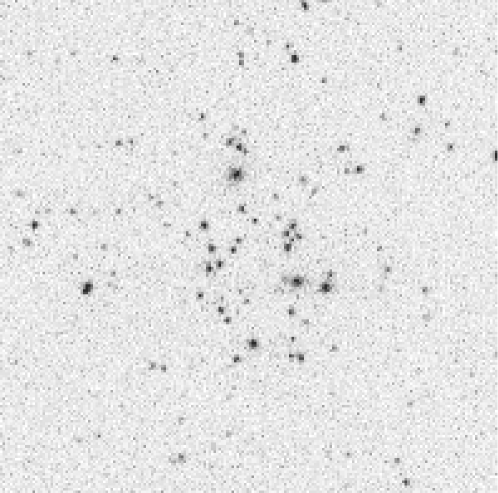
In Figure 1, we show an example of a high redshift cluster detected in this preliminary catalog, while in Figure 2, we show a very preliminary determination of the SRC X–ray Cluster Luminosity Function (XCLF) (21 clusters above $L_{\rm ROSAT}(44)>1$ in the redshift range $0.0<z<0.45$). Here we have used runs 752 & 756 ($213\,{\rm deg^{2}}$) and 94 & 125 ($90\,{\rm deg^{2}}$) from the SDSS data (see York et al. 2000) which we have naively assumed to be complete to a flux limit of $4$ and $8\times 10^{-13}\,{\rm erg/s/cm^{2}}$ respectively. This assumption is valid for our luminous clusters but breaks down for lower luminous clusters and undoubtedly accounts for the “low” data points in our XCLF at $L_{\rm ROSAT}(44)\sim 1$. We have also conservatively cut the catalog at $z<0.45$ and removed suspicious match–ups by hand (see Sheldon et al. 2000). However, the SRC does have candidate $z\simeq 0.7$ clusters which will require spectroscopic confirmation (Annis et al. 2000).

We present this data to illustrate the power of the SRC for detecting real clusters to high redshift; the combination of these two, large area, catalogs (SDSS and RASS) allows us to push to fainter fluxes (and thus higher redshift) than one would be able with either survey on its own. Finally, the XCLF presented here is fully consistent with other measurements and adds new information regarding the existence of a “deficit” of high redshift, high luminosity clusters which has been debated by many authors (e.g. Reichart et al. 1999; Nichol et al. 1999; Gioia et al. 1999). This is because the SRC covers a large area of sky ($\simeq 300{\rm deg^{2}}$ at present) which is vital for detecting massive, X–ray bright clusters at high redshift (see Ebeling et al. 2000).

Figure 2: We show here a preliminary XCLF for the SRC survey ($0.0<z<0.45$; stars). The shaded region is the local ($0.0<z<0.3$) x-ray luminosity function, plus $1\sigma$ errors, as measured by de Grandi et al (1999) and Ebeling et al (1998). The circles are the SHARC ($0.3<z<0.7$ Burke et al. 1997; Nichol et al. 1999). Poisson errors are shown.

3 Finding Clusters in Multiple Dimensions

Over the last few years, there has been significant progress in the development of new cluster–finding algorithms primarily driven by the quality and quantity of new data as well as the increased availability of fast computing. These new methods include the matched–filter algorithm (Postman et al. 1996, Kawasaki et al 1998, Kepner et al 1999, Bramel et al. 2000), the wavelet–filter (Slezak et al 1990), the “photometric redshift” method (Kodama et al. 1999), and the “density–morphology” relationship (Ostrander et al. 1998) or the E/S0 ridge–line (Gladders & Yee 2000).

Here we outline a new algorithm we have developed which exploits the quality and quantity of data available to us. For instance, the SDSS will provide accurate, calibrated magnitudes in 5 filters ($u^{{}^{\prime}}g^{{}^{\prime}},r^{{}^{\prime}},i^{{}^{\prime}},$ and $z^{{}^{\prime}}$) as well as accurate star-galaxy separation, galaxy shapes, photometric redshifts and estimates of the galaxy type. These increased number of observables allow us to refine our definition of a cluster to be an overdensity of galaxies in both space (on the sky and in redshift) and rest–frame color. Furthermore, we can require that the cluster members be early–type galaxies and that the cluster, as a whole, is coincident with extended hard X-ray emission. The motivation for this definition of a cluster is the growing body of evidence that the cores of clusters are dominated by ellipticals of the same colors suggesting they are coeval (see Gladders & Yee 2000), and possess a hot, intracluster medium (see Holden et al. 2000). Via this definition, we can radically increase the signal–to–noise of clusters in this multi–dimensional space thus effectively removing projection effects and X–ray mis–identifications which presently plague optical and X–ray cluster surveys respectively. We have nicknamed this algorithm “C4” for 4–color clustering.

We note that this definition may bias us against certain types of clusters e.g. young systems where the X–ray gas may be more diffuse (thus a lower emissivity) and/or have a bluer, less homogeneous, galaxy population. However, over the redshift range probed by SDSS & RASS ($z<0.8$), most clusters are expected to be well evolved since they have formation epochs of $z\geq 2$. Moreover, we will need to quantify our exact selection function regardless of the algorithm used (see Section 3.4).

We present here a brief overview of the C4 algorithm and then present specific details about parts of the algorithm below. We start by considering galaxy $X_{i}$ which is any detected galaxy with a known or photometric redshift. The fundamental question the C4 cluster-finding algorithm poses is: Is there an overdensity of cluster-like galaxies about galaxy $X_{i}$? Our solution for answering this question is rather simple. First, we count $N_{i}$, the number of galaxies in a multi–dimensional aperture around galaxy $X_{i}$. The aperture (discussed in detail in Section 3.1) is defined in angular, redshift and color space. Second, for each test galaxy $X_{i}$, we measure a field distribution, $F(X_{i})$, which is constructed via Monte Carlo realisations of placing the same size aperture as the test galaxy on thousands of randomly chosen galaxies in regions of similar extinction and seeing as $X_{i}$. Third, if galaxy $X_{i}$ is in a clustered region, then $N_{i}$ will lie in the tail of the distribution and we can measure a probability, $p_{i}$, that galaxy $X_{i}$ is a member of this field distribution $F(X_{i})$. We then have to decide what acceptable cut-off in $p_{i}$ differentiates between cluster galaxies and field galaxies (see Section 3.2). Note that C4 does not find clusters but detects cluster–like galaxies. It is based on a well-defined description of the field, which is easily measured from a large-volume survey such as the SDSS. Those galaxies that have a low probability of being a field galaxy are then considered to be cluster members. Finally, we use these cluster–like galaxies to locate the positions of the actual clusters in the data.

Figure 3: The distribution of $p$–values for the 183 galaxies within the aperture of SRC galaxy RXJ0254 (Figure 1). Inserted is a blow–up of small $p$–values which illustrates the strong peak near zero i.e. probability in 6–dimensional space that these galaxies were drawn from the field distribution. This illustrates the strength of clustering one can obtain since 6–dimensional space is mostly empty and thus finding any grouping of galaxies on the sky with the same redshift & color is enough to make it highly unlikely that they are drawn from a random field population.

3.1 Choosing The Aperture: Shape Doesn’t Matter

A critical part of computing $N_{i}$ – the galaxy count in multi–dimensions around our test galaxy – is the choice of the size and shape of the counting aperture i.e. we are using a kernel to smooth the data. We note here that we focus on defining the width of this kernel or aperture, rather than the shape, since it is well–known in the statistical literature that the choice of bandwidth of a kernel is more important when optimally smoothing data than the exact shape of that kernel.

To discuss this further, suppose that $X_{1},\ldots,X_{n}$ are independent observations from a probability density function $f(x)$. A common estimator is the kernel estimator defined by

$$\hat{f}(x)=\frac{1}{n}\sum_{i=1}^{n}\frac{1}{h_{n}}K\left(\frac{x-X_{i}}{h_{n}}\right).$$

The function $K$ is called the kernel and is usually assumed to satisfy $K(x)\geq 0$, $\int K(x)dx=1$, $\int xK(x)dx=0$. For example, the Gaussian kernel is $K(x)=\{2\pi\}^{-1/2}e^{-x^{2}/2}$. The number $h_{n}$ is the bandwidth and controls the amount of smoothing. One can see from numerical experimentation that the choice of $K$ has very little effect on the estimator $\hat{f}$ but the choice of $h_{n}$ has a drastic effect. This can also be proved mathematically. For example, consider the integrated means squared error (IMSE) defined by

$$IMSE=E\int(f(x)-\hat{f}(x))^{2}dx$$

where $E$ is the average or expectation value. One can derive an analytic expression for IMSE and from this expression one sees that $K$ has little effect on IMSE but $h_{n}$ has a drastic effect. Details are given in Density Estimation for Statistics and Data Analysis by Silverman (1986). In fact, one can show that the optimal kernel, which minimizes IMSE, is given by $K(x)=(3/4)(1-t^{2}/5)/\sqrt{5}$ for $|x|<\sqrt{5}$ and 0 otherwise. This is called the Epanechnikov kernel. But the efficiency of other kernels (the ratio of the IMSEs) is typically near 1. For example, the Gaussian kernel has an efficiency of 0.95 compared to an Epanechnikov kernel. In contrast, the effect of $h_{n}$ is dramatic, so; how does one find the optimal bandwidth? This is clearly difficult and in statistics, it is usually achieved using “cross-validation” where one estimates the $IMSE(h_{n})$ and finds $h_{n}$ to minimize this function (see Silverman 1986).

Therefore, we simply use a top–hat kernel in the C4 algorithm and use the known observables of the galaxy $X_{i}$ (redshift and colors), as well as known physical relationships, to define the aperture size or bandwidth. We start by defining an input mass scale to search for clusters. This allows us to calculate $r_{200}$ which is converted to an angular aperture ($\Delta\theta$) as function of cosmology. In this conversion, we use either the known or photometric redshift (see Connolly et al. 1995). Next we define a redshift aperture, $\Delta z$, which is based on the expected radial velocity dispersion for a cluster with $r_{200}$ (determined analytically). This is also convolved with the error on the observed or photometric $z$. Finally, we use a 4-dimensional color-aperture, $\Delta_{i}c$, for $i=1,4$, where the width of this aperture is simply the measured errors on the SDSS photometric magnitudes for galaxy $X_{i}$.

Once we have defined our aperture, we then simply count the number of neighboring galaxies within this 6–dimensional aperture. We note that all the SDSS galaxies will possess errors on the redshift (photometric and spectroscopic) and colors, so instead of counting each galaxy as a single delta–function in our count $N_{i}$, we can treat each galaxy as an error ellipsoids in 6–dimensional space and compute the amount of overlap between these ellipsoids and the aperture. This is non-trivial and therefore, we will Monte Carlo the effect by computing many $N_{i}$ around each test galaxy $X_{i}$ perturbing in each case the surrounding galaxies by their observed errors. This will result in a distribution of $N_{i}$ for each galaxy, $f(N_{i})$.

The counting queries we have outlined above are computationally intensive and thus, to make this problem tractable, we will exploit the emerging algorithmic technology of multi–resolutional KD–trees (see Connolly et al. 2000) which can scale as $N\,logN$, instead of $N^{2}$, for range searches like those discussed herein. We defer discussion of these computational issues to a forthcoming paper.

Having measured $N_{i}$, we now need to build the field distribution, $F(X_{i})$. Recall, we want to use the same size aperture as that of galaxy $X_{i}$. In order to determine $F(X_{i})$, we will count galaxies around a random distribution of galaxies that lie in regions of similar extinction and seeing to that of galaxy $X_{i}$. As above, these field counts can be corrected for observational errors and thus $F(X_{i})$ will be the sum of many count distributions around each randomly selected field galaxy.

Figure 4: (Top left) A $3^{\circ}\times 3^{\circ}$ area from SDSS photometric data runs 752 & 756 (rerun 1). We show all galaxies regardless of redshift, color or magnitude. (Top right) This is the result of running the C4 algorithm on this data using a 5% FDR threshold. We rejected 4% of the galaxies on the left as being field–like galaxies. (Bottom) Same area taken from the RASS hard photon data (each dot is at least one photon). The large cluster seen in the field is Abell 1882 (richness class 3 and $z=0.137$). The axes are RA and DEC

3.2 Choosing The Threshold: False Discovery Rate

Once we have $N_{i}$ and $F(X_{i})$ for each test galaxy $X_{i}$, we can compute the probability, or $p$–value, that this test galaxy was drawn from the field. This is achieved by fitting a Poisson distribution to the lower end of the $F(X_{i})$ distribution (which must be the field population) and comparing $N_{i}$ to that fitted distribution, see Figure 3.

In this process, we can make two types of errors: (1) falsely identifying a real field galaxy as cluster-like (false rejection); (2) falsely identfiying a real cluster galaxy as field like (false non-rejection). The next critical decision is to determine the $p$-cutoff below which a galaxy is rejected as being field–like.

This threshold could be chosen arbitrarily. For instance, for each test we could apply a $2\sigma$ confidence requirement and reject any galaxy with $p<0.05$. However, after $N_{totalgalaxies}=1million$ tests, we would expect to have made as many as 50000 mistakes through false rejections. This is far too many mistakes which could be reduced by applying a higher confidence requirement e.g. $4\sigma\rightarrow p_{cutoff}=3\times 10^{-7}$. This leads to the traditional approach of permitting no false rejections with 95% confidence through lowering the $p$-cutoff to $0.05/N_{gal}$ where $N_{gal}$ is the number of test galaxies. This is known as the Bonferoni Method where each individual test is very conservative to allow for no false rejections. The disadvantage of this approach is that a lot of cluster–like galaxies would be mis-classified as field–like (i.e. false non-rejections) since we have enforced a very strict limit on the number of field–like galaxies that are allowed to be mis–classified as cluster–like galaxies. This is an extreme case where one sacrifices errors in one direction for the control of mis–classification errors in the opposite direction. If there were no cluster–like galaxies in our test sample of galaxies, then the Bonferoni Method would be correct, however $\sim 20$% of all galaxies live in cluster & group environments, so if we using this method we would loose significant sensitivity to detecting these galaxies.

Instead of either of the above two thresholding techniques, we use the newly devised False Discovery Rate (FDR; Abramovich et al. 2000). FDR is a new, more adaptive approach which, in the limit of all the galaxies in the test sample being field–like, would be equivalent to the Bonferoni Method. However, FDR becomes less conservative, and makes fewer errors in the other direction, as we diverge from this idealized case. In practical terms, FDR allows us to define in advance a desired false detection rate i.e. up–front only $\alpha\times 100\%$ of the rejected galaxies are in error based on our null hypothesis. Moreover, the FDR procedure is simple:

1. For each test galaxy, calculate a $p$-value based on the null hypothesis that it is a field galaxy.

2. Sort these according to increasing $p$-value.

3. Rank the $p$-values as a function of $n/N$ where $n$ is the $n^{th}$ galaxy’s $p$-value out of $N$ total test galaxies.

4. Draw a line with slope ($\alpha$) and intercept 0.

5. From the right, determine the first crossing of the line with the ranked $p$-values.

6. Anything with a $p$-value smaller than the crossing $p$-value is rejected.

7. For our cluster–finding algorithm, these rejected galaxies are our cluster–like galaxies, with at most $\alpha\times 100\%$ errors based on our null field galaxy hypothesis.

The beauty of FDR is that (a) it is simple, (b) it possesses a rigorous statistical proof, and (c) it works for highly correlated data (in this case the slope becomes $\alpha/{\rm log}N$). In summary, FDR is a new tool in statistics which has the potential to significantly enhance astronomical analyses; this is the first application of this new statistic in astronomy and demonstrates the power of our “Computational AstroStatistics” collaboration. Other possible applications could be determining the sky threshold values in source detection, point–source extraction in CMB analyses etc. We will explore these application in a forthcoming paper.

3.3 Clustering Cluster–like Galaxies

In Figure 4, we show the results of running our C4 algorithm, with FDR, on the SDSS commissioning photometric data (York et al. 2000). The next task is to “cluster” these cluster–like galaxies into a sample of unique clusters of galaxies. To do this, we employ the Expectation Maximization (EM) algorithm which is a mixture model of Gaussians designed to be highly adaptive and multi–resolutional in nature. Moreover, it is naturally multi–dimensional thus allowing us to feed it three galaxy spatial coordinates (angular position and redshift) as well as three X–ray dimensions (hard photon energy and angular position). The rational for jointly clustering the X–ray and optical data is to drastically increase the signal–to–noise of distant and poor clusters by suppressing projection effects and X–ray mis–identifications. The details of mixture–model clustering and the EM algorithm can be found in Connolly et al. (2000). In addition, to using EM we plan to investigate adaptive kernel density estimators. We note here that during the clustering process additional information can be used to “mark” or “up–weight” galaxies. For example, SDSS data can be used to determine if a galaxy is elliptical–like based on the imaging morphology (likelihood fits to each galaxy for both a da Vaucouleurs and exponential profile), photometric spectral classification information of Connolly & Szalay (1999) as well as spectral classifications where available (see Castander et al. 2000 for details).

3.4 The Selection Function & Systematic Biases

The most direct method of quantifying the selection function of our SDSS cluster catalog is via Monte Carlo simulations (see Bramel et al. 2000; Kim et al.2000). These simulations can then be converted to an effective area, or volume, of the survey as a function of the input cluster parameters (redshift, luminosity etc). In addition to simulations, we can obtain information about the selection function of the various SDSS cluster catalogs (Annis et al. 2000; Kim et al. 2000) by cross-correlating them against each other and the low redshift SDSS galaxy redshift survey. These different SDSS cluster catalogs use different cluster selection criteria since they are explore different science issues and are therefore, complementary.

In summary, we have outline here our new C4 cluster–finding algorithm that exploits the quality and quantity of the multi–dimensional survey data now becoming available. It also exploits new techniques and algorithms coming out of Computer Science and Statistics. We plan to jointly “cluster” optical and X–ray data to help improve the signal–to–noise of distant and/or poor clusters/groups of galaxies. This represents a first step toward the “Virtual Observatory”; the joint scientific analysis of archival multi–wavelength survey databases. The algorithms and software we develop will become part of the “Virtual Observatory” analysis toolkit.

References

- [1] Adami, C. et al. 2000, ApJ, see astro-ph/0007289
- [2] Annis, J., 1999, BAAS, 195
- [3] Abramovich, F. et al. 2000 (Technical Report, Stanford Stats)
- [4] Bahcall, N.A., Fan, X., & Cen, R. 1997, ApJL, 485, 53
- [5] Borgani, S., Rosati, P., Tozzi, P., & Norman, C. 1999, ApJ, 517, 40.
- [6] Bramel, D. A., Nichol, R. C., Pope, A., 2000, ApJ, 533, 601
- [7] Burke, D. J., et al., 1997, ApJ, 488, 83
- [8] Castander, F. J., et al., 2000, AJ, (see astro-ph/0010470)
- [9] Collins, C. A., et al., 2000, see astro-ph/0008245
- [10] Connolly, A. J., et al. 1995, AJ, 110, 2655
- [11] Connolly, A. J. & Szalay, A. S. 1999, AJ, 117, 2052
- [12] Connolly, A. J., et al. 2000, AJ, submitted see astro-ph/0008187
- [13] de Grandi, S., et al., ApJ, 513, 17
- [14] Ebeling, H., et al., 1997, MNRAS, 301, 881.
- [15] Ebeling, H., Edge, A.C., Henry, J. P., 2000, see astro-ph/0001320
- [16] Eke, V. R., Cole, S., Carlos, F., & Henry, J. P., 1998, MNRAS, 298, 1145
- [17] Gioia, I. A., et al., 1999, see astro-ph/9902277
- [18] Gladders, M. D., Yee, H., 2000, AJ, see astro-ph/0004092
- [19] Henry, J.P. 1997, ApJ, 489, L1.
- [20] Holden, B. P. et al. 2000, AJ, 120, 23
- [21] Kawasaki, W., Shimasaku, K., Doi, M., Okamura, S., 1998, A&AS, 130, 567
- [22] Kepner, J., et al., 1999, ApJ, 517, 78
- [23] Kim, R. et al. 2000, AJ, in prep.
- [24] Kodama, T., Bell, E. F. & Bower, R. G. 1999, MNRAS, 302, 152
- [25] Kron, R., 1993, “The Deep Universe”, Saas–Fee Lectures Notes
- [26] Ostrander, E. J., et al., 1998, AJ, 116, 2644
- [27] Postman, M.P., et al., 1996, AJ, 111, 615
- [28] Press, W. H., & Schechter, P. 1974, ApJ, 187, 425
- [29] Nichol, R. C., et al., 1999, ApJL, 481, 644
- [30] Nichol, R. C., et al., 2000, proceedings from Virtual Observatories of the Future, Brunner& Szalay (astro-ph/0007404)
- [31] Reichart, D.E., et al., 1999, ApJ, 518, 521
- [32] Romer, A. K., Viana, P., Liddle. A., Mann, R. G., 2000, ApJ, astro-ph/9911499
- [33] Sadat, R., Blanchard, A., & Oukbir, J., A&A, 329, 21
- [34] Sheldon, E., et al., 2000, BAAS, 196
- [35] Slezak, E., et al., 1990, A&A, 227, 301
- [36] Viana, P. T. P. & Liddle, A. R. 1999, MNRAS, 303, 535
- [37] Voges, W., et al., 2000, IAU Circ., 7432, 3
- [38] York, D., et al., 2000, AJ, in press (see astro-ph/0006396)