*

Abstract

We present an overview of the upcoming Microwave Anisotropy Probe (MAP) mission, with an emphasis on those aspects of the mission that simplify the data analysis. The method used to make sky maps from the differential temperature data is reviewed and we present some of the noise properties expected from these maps. An overview of the method we plan to use to mine the angular power spectrum from the mega-pixel sky maps closes the paper.

1 Mission Overview

In 1992 NASA’s Cosmic Background Explorer (COBE) satellite made a full sky map of the cosmic microwave background (CMB) temperature with 7^∘ resolution, uncorrelated pixel noise, minimal systematic errors, and accurate calibration, from which CMB temperature anisotropy was first discovered [1], [2], [3], [4]. The purpose of the MAP mission is to re-map the anisotropy over the full sky with more than 30 times the angular resolution ($\sim 0.23^{\circ}$ FWHM) and more than 35 times the sensitivity ($\sim 20$ $\mu$K per 0.3^∘ pixel) of COBE, but with the same level of quality control as was possible with COBE. With this data, MAP will measure the physical interactions of the photon-baryon fluid (sound waves) in the early universe and thereby test models of structure formation, the geometry of the universe, and inflation.

In the years since COBE, a host of ground-based and balloon-borne experiments have detected and characterized fluctuations at smaller angular scales, most recently the experiments TOCO [5], BOOMERanG [6] and MAXIMA [7]. However, because of their proximity to the Earth and its atmosphere, none of the ground or balloon-based experiments enjoy the extent of systematic error rejection or calibration accuracy that was possible with COBE. Moreover, many of these experiments have significantly correlated noise that places severe demands on the data analysis. The COBE data still serves as a benchmark for the field and many aspects of the COBE mission have influenced the design of the MAP mission. The need to minimize the level of systematic errors has been the major driver of the MAP design and has led to the following high level design features:

• A highly symmetric differential design: MAP is a differential experiment based on pseudo-correlation microwave radiometers that employ phase-matched HEMT amplifiers. The instrument measures temperature differences between two points $\sim$ 141^∘ apart on the sky. By measuring temperature differences, rather than absolute temperatures, many spurious signals will be common-mode and thus cancel upon differencing. Also, by employing a pseudo-correlation design with a fast chopping frequency between the two sky inputs, 1/f noise that arises from the HEMTs can be chopped out. The resulting power spectrum of the radiometer noise is very nearly white (see §3).

• Multi-frequency: There are five frequency bands from 22-90 GHz that will allow emission from the Galaxy and other non-cosmological sources to be modeled and removed based on their frequency dependence. In the lowest frequency bands, MAP will probe the high frequency tail of radio emission from our Galaxy and provide valuable data on the enigmatic microwave foreground emission that correlates with thermal dust emission, but has a much different spectrum. See [8] for a recent summary of evidence for this foreground.

• Stability: MAP will observe from a Lissajous orbit about the L2 Lagrange point 1.5 million km from Earth. The L2 point offers an exceptionally stable environment and an unobstructed view of deep space, with the Sun, Earth, and Moon always in shadow behind MAP’s Sun shield. MAP’s large distance from Earth protects it from near-Earth emission and other disturbances. While observing at L2, MAP’s Sun shield and solar panels maintain a fixed angle with respect to the Sun to provide exceptional thermal and power stability.

• Low beam sidelobe levels: The MAP optical system was designed with the foremost goal of providing adequate angular resolution along the line of sight while at the same time rejecting stray light from other directions. For example, the largest instantaneous signal due to radiation from the galactic plane spilling into a sidelobe is expected to be less than 2 $\mu$K at 90 GHz.

An overview of the MAP satellite is shown in Fig. 1. The major visible features of MAP include the back-to-back telescope optics with 1.4 $\times$ 1.6 m primary mirrors and 1 m secondary mirrors, the passive thermal radiators which cool the HEMT amplifiers to $<$100 K, the hexagonal structure housing the spacecraft service modules, and the large solar panel array/Sun shield which keeps the instrument in full shade. MAP weighs a total of 830 kg and stands $\sim$4 m tall. It will be launched in 2001 aboard a Delta 7425-10 expendable launch vehicle from the NASA Kennedy Space Center Eastern Test Range.

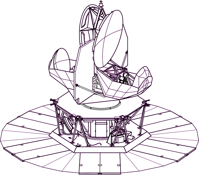
Figure 1: An overview of the MAP satellite.

2 Scan Strategy

The MAP scan strategy plays an important role in systematic error rejection. It was designed with the following goals in mind:

• Scan a large fraction of the sky as rapidly as possible, consistent with reasonable requirements on the controlling hardware and the telemetry data rate.

• Scan each sky pixel through as many azimuthal angles as possible for the reasons listed below.

• Observe a given pixel on as many different time scales as possible.

• Maintain the instrument in continuous shadow for optimal passive cooling and avoidance of stray signals from the Sun, Earth, and Moon.

• Maintain a constant angle between the Sun and the plane of the solar panels for thermal and power stability.

The strategy that was ultimately adopted combines a “fast” spin about the spacecraft symmetry axis with a slow precession about the Sun-MAP line (which is always within 0.1^∘ of the Sun-Earth line at L2). Since each telescope line of sight is $\sim 70^{\circ}$ off the symmetry axis, the path swept out on the sky by a given line of sight resembles a spirograph pattern that reaches from the north to south ecliptic poles. As MAP orbits the Sun, this pattern revolves around the sky so that full sky coverage is first achieved after 6 months of observing at L2.

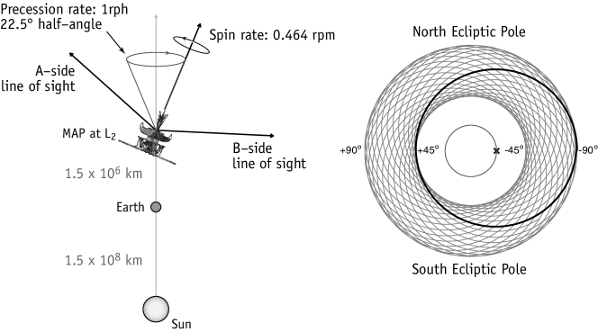
Figure 2: A schematic of the MAP scan strategy from L2. The satellite covers approximately 35% of the sky each day. The scan pattern on the right depicts the motion of a single line of sight over a 1 hour precession period (lighter spirograph pattern), and a $\sim$2 minute spin period (darker single circle). The inner circle depicts the path of the spin axis during one precession.

The MAP scan strategy achieves a reasonable level of azimuthal coverage in each sky pixel. For example, a pixel in the ecliptic equator is observed over $\sim$30% of the possible angles of attack; a pixel at the cusp of the annular coverage at $\sim 45^{\circ}$ ecliptic latitude is observed over about 70% of possible angles of attack; and a pixel near the ecliptic poles is observed from 100% of the possible azimuthal orientations. A large azimuthal coverage provides numerous desirable features in the data:

• Helps to produce a stable sky map solution.

• Produces small pixel-pixel covariance at the beam separation scale.

• Minimizes striping due to any residual 1/f noise in the differential data.

• Maximizes polarization sensitivity.

• Maximizes azimuthal symmetry of the beam response on the sky.

From this standpoint, the MAP strategy is not as complete as COBE’s, which achieved nearly 100% azimuthal coverage in all pixels. However, in order to achieve such completeness, the spacecraft spin axis must ultimately point to every pixel on the sky which is less desirable from the standpoint of systematic error avoidance. The MAP strategy achieves reasonable azimuthal coverage consistent with strong systematic error constraints. Extensive simulations of the map making and power spectrum estimation procedures have shown that the strategy is more than adequate to meet MAP’s scientific goals.

3 Map Making with Differential Data

Sky maps, ${\bf t}$, are obtained from the differential data, ${\bf d}$, by linear least squares fitting. The raw data takes the form ${\bf d}={\bf A}\cdot{\bf t}$ where ${\bf A}$ is the scan matrix of the experiment which has $N_{pix}$ columns and $N_{obs}$ rows, where $N_{pix}$ is the number of sky map pixels and $N_{obs}$ is the total number of differential observations.

Each row (observation) of length $N_{pix}$ contains a $+1$ in the element (pixel) observed by the $+$ horn during that observation, and a $-1$ in the element observed by the $-$ horn. The normal equations for the sky map solution are

$$({\bf A}^{T}\cdot{\bf T}^{-1}\cdot{\bf A})\cdot{\bf t}={\bf A}^{T}\cdot{\bf T}^{-1}\cdot{\bf d}$$ (1)

where ${\bf T}$ is the covariance of the instrument noise in the time domain. For MAP’s differential radiometers this is well approximated by stationary, white noise, $T_{tt^{\prime}}=\langle n_{t}n_{t^{\prime}}\rangle\approx\sigma_{0}^{2}\delta_{tt^{\prime}}$. A sample of the MAP noise covariance is shown in Fig. 3 from test data taken with the flight instrument. The whiteness of the noise greatly simplifies the subsequent data processing and analysis for two reasons 1) the normal equations for the sky map are much easier to solve than they would be with significant 1/f noise, 2) the pixel-pixel noise covariance in the final sky maps is very small and completely negligible for most applications.

Figure 3: The auto-correlation function (denoted ${\bf T}$ in the text) of 8 hours of noise from one of the MAP 90 GHz radiometers, taken during a cold instrument test in March 2000. The instrument was operating at expected flight temperature while observing temperature controlled targets over the flight feeds. The only processing applied to the raw data was to subtract a baseline with power on periods of greater than  1 hour (a Legendre polynomial of order 8 fit over the 8 hour period of data). This approximates the procedure that will be applied to the flight data. Note the point at lag 1 (inset) has a covariance of 1.2% of the raw noise due to a low-pass filter applied just prior to the a/d conversion. There is no other significant covariance in the noise.

With stationary white noise, the maximum likelihood sky map solution reduces to

$${\bf t}=({\bf A}^{T}\cdot{\bf A})^{-1}\cdot({\bf A}^{T}\cdot{\bf d})$$ (2)

while the pixel-pixel noise covariance is

$${\bf N}=\sigma_{0}^{2}\,({\bf A}^{T}\cdot{\bf A})^{-1}.$$ (3)

Formally, the sky map solution (2) requires inverting an $N_{pix}\times N_{pix}$ matrix ${\bf M}\equiv({\bf A}^{T}\cdot{\bf A})$ which has the form

$${\bf M}=\left(\begin{array}[]{rrrrrrrr}N_{0}&0&0&\cdots&-N_{0i}&0&0&\cdots\\ 0&N_{1}&0&\cdots&0&-N_{1j}&0&\cdots\\ 0&0&N_{2}&\cdots&0&0&-N_{2k}&\cdots\\ \vdots&\vdots&\vdots&\vdots&\vdots&\vdots&\vdots&\ddots\\ -N_{0i}&0&0&\cdots&N_{i}&0&0&\cdots\\ 0&-N_{1j}&0&\cdots&0&N_{j}&0&\cdots\\ 0&0&-N_{2k}&\cdots&0&0&N_{k}&\cdots\end{array}\right)$$ (4)

where the $i$th diagonal element is the number of times pixel $i$ was observed by either side of the instrument, and the $ij$th off-diagonal element is the number of times pixels $i$ and $j$ were observed simultaneously. Because of the fixed separation between the two instrument beams, only pairs of pixels separated by a fixed distance can be simultaneously observed, thus this matrix is very sparse. Furthermore, because the scan strategy generates ample azimuthal coverage, we have $N_{ij}\ll N_{i}$ so ${\bf M}$ is diagonally dominant. [Formally ${\bf M}$ is singular because the sum of each of its rows or columns is zero, due to the fact that the time-series data is differential. Thus the sky map solution and its pixel-pixel covariance are undetermined up to a constant since ${\bf M}\cdot{\bf C}=0$ for any constant vector or matrix ${\bf C}$. In practice this mode is readily projected out of the data in any actual inversion scheme.]

The form of ${\bf M}$ suggests an iterative approach to solving for the map that employs a diagonal pre-conditioner as an approximate inverse [9]. Define

$$\tilde{\bf M}^{-1}=\mbox{diag}(\frac{1}{N_{0}},\frac{1}{N_{1}},\frac{1}{N_{2}},\ldots)$$ (5)

and assume an approximate initial map solution ${\bf t}_{0}={\bf t}+\delta{\bf t}$ such that

$${\bf M}\cdot{\bf t}_{0}={\bf M}\cdot({\bf t}+\delta{\bf t})={\bf v}+\delta{\bf v}$$ (6)

where ${\bf v}\equiv{\bf A}^{T}\cdot{\bf d}$. This gives an expression for $\delta{\bf t}$ in terms of known quantities

$${\bf M}\cdot\delta{\bf t}={\bf M}\cdot{\bf t}_{0}-{\bf v}$$ (7)

We can use the above pre-conditioner to obtain an iterative estimate of the map correction $\delta{\bf t}_{1}$, and hence an improved solution ${\bf t}_{1}$

$${\bf t}_{1}={\bf t}_{0}-\delta{\bf t}_{1}={\bf t}_{0}-\tilde{{\bf M}}^{-1}\cdot({\bf M}\cdot{\bf t}_{0}-{\bf v}).$$ (8)

As was noted in [10], an efficient way to evaluate the right hand side of (8) is to group the operations as follows

$${\bf t}_{n+1}=(\tilde{{\bf M}}^{-1}\cdot{\bf A}^{T})\cdot({\bf d}-{\bf A}\cdot{\bf t}_{n})+{\bf t}_{n}.$$ (9)

The interpretation of (9) is that for each pixel the new sky map temperature is equal the average of all differential observations of that pixel, accounting for the sign of the observing horn, corrected by an estimate of the signal in the pair horn, based on the previous sky map iteration. The expression in (9) can be efficiently evaluated because the sums can be accumulated by reading through the time-series data, read from disk, and accumulating data into arrays of length $N_{pix}$. It is never necessary to store or invert and $N_{pix}\times N_{pix}$ matrix.

Figure 4: 2-point angular correlation function of a simulated MAP noise map. The function was computed from a residual sky map that was obtained by subtracting an input sky map from a solution of the map-making algorithm. The noise used in the simulated differential data was statistically identical to the actual radiometer test data shown in Fig. 3. Note the small ($<$1%) nearest-neighbor covariance due to the nearest-neighbor covariance in the time-series data. There is also a small ($\sim$0.1%) covariance between pixels separated by the beam spacing, indicated by the dashed line in the inset panel.

The performance of this algorithm has been tested extensively with simulations that capture differential data with realistic instrument noise observed with the MAP scan strategy. The solution is seen to converge to the input in less than 50 iterations, starting from an initial guess with no anisotropy. In cases where the instrument noise has been suppressed for study purposes, peak-peak features in the residual sky map (output $-$ input) are less than 0.1 $\mu$K. In cases where realistic noise is included, the performance of the algorithm can be measured by the 2-point angular correlation function of the residual (noise) map. Ideally, this would be everywhere consistent with zero except for the bin at zero angular separation which should equal the variance of the map. Fig. 4 shows the 2-point function obtained from a noise map that was obtained from the MAP algorithm. To a very good approximation, the noise in the sky map is uncorrelated from pixel to pixel.

4 Power Spectrum Estimation from Full Sky Maps

The most fundamental statistic to measure from the observed sky map is its angular power spectrum, $C_{\ell}$, which measures the variance of the fluctuations over a range of angular scales. If the temperature fluctuations are gaussian, and the a priori probability of a given set of cosmological parameters is uniform, then the power spectrum may be estimated by maximizing the multi-variate gaussian likelihood function

$${\cal L}(C_{\ell}|{\bf m})=\frac{\exp(-\frac{1}{2}{\bf m}^{T}\cdot{\bf C}^{-1}\cdot{\bf m})}{\sqrt{\det{\bf C}}}$$ (10)

where ${\bf m}$ is a data vector (see below) and ${\bf C}$ is the covariance matrix of the data which has contributions from both the signal and the instrument noise, ${\bf C}={\bf S}+{\bf N}$. We can work in whatever basis is most convenient, in the pixel basis the data are the sky map pixel temperatures while in the spherical harmonic basis the data are the $a_{\ell m}$ coefficients of the map. In the former basis the noise covariance is nearly diagonal, while in the latter, the signal covariance is

$$\begin{array}[]{lllp{5mm}lll}&&\mbox{Pixel basis:}&&&&\mbox{Spherical harmonic basis:}\\[5.69054pt] {\bf m}&\rightarrow&T_{i}&&{\bf m}&\rightarrow&a_{\ell m}\\[5.69054pt] {\bf S}&\rightarrow&\sum_{\ell}\frac{(2\ell+1)}{4\pi}C_{\ell}P_{\ell}(\cos\theta_{ij})&&{\bf S}&\rightarrow&{\rm diag}(C_{2},C_{2},\ldots C_{3},C_{3},\ldots)\\[5.69054pt] {\bf N}&\rightarrow&\sigma_{i}^{2}\delta_{ij}&&{\bf N}&\rightarrow&N_{(\ell m)(\ell m)^{\prime}}\mbox{(see below)}.\end{array}$$

In the case of MAP, the length of the data vector, $N_{data}$, is of order 1 million, so it is necessary to find methods for evaluating ${\cal L}$ that do not require a full inversion of the covariance matrix ${\bf C}$, which requires $O(N_{data}^{3})$ operations. As with the map-making, our approach is fundamentally an iterative one that exploits the ability to find an approximate inverse $\tilde{\bf C}^{-1}$. The most important feature in the data that makes this possible is the fact that we cover the full sky and that the galaxy cut we impose on the data is predominantly azimuthally symmetric in galactic coordinates. Of secondary importance for this pre-conditioner is that fact that our noise per pixel is not too strongly varying across the sky. We discuss the pre-conditioner in more detail below.

We maximize the likelihood by solving

$$\begin{array}[]{lp{5mm}l}\frac{\partial f}{\partial C_{\ell}}=0={\bf m}^{T}\cdot{\bf C}^{-1}\cdot{\bf P}^{\ell}\cdot{\bf C}^{-1}\cdot{\bf m}+{\rm tr}({\bf C}^{-1}\cdot{\bf P}^{\ell})&&f\equiv-2\ln{\cal L}\\[5.69054pt] &&{\bf P}^{\ell}\equiv\frac{\partial{\bf C}}{\partial C_{\ell}}\end{array}$$ (11)

using a Newton-Raphson approach to root finding that generates an iterative estimate of the angular power spectrum at each step

$$C_{\ell}^{(n+1)}=C_{\ell}^{(n)}-\frac{1}{2}\sum_{\ell^{\prime}}F_{\ell\ell^{\prime}}\frac{\partial f}{\partial C_{\ell}}$$ (12)

where $F_{\ell\ell^{\prime}}$ is the Fisher matrix

$$F_{\ell\ell^{\prime}}=\langle-\left(\frac{\partial^{2}}{\partial C_{\ell}\partial C_{\ell^{\prime}}}\right)\ln{\cal L}\rangle=\frac{1}{2}{\rm tr}({\bf C}^{-1}\cdot{\bf P}^{\ell}\cdot{\bf C}^{-1}\cdot{\bf P}^{\ell^{\prime}}).$$ (13)

In order to implement the solution in (12) we need to be able to evaluate the following components of $\sum_{\ell^{\prime}}F_{\ell\ell^{\prime}}\frac{\partial f}{\partial C_{\ell}}$ quickly

$$\begin{array}[]{l}{\bf m}^{T}\cdot{\bf C}^{-1}\cdot{\bf P}^{\ell}\cdot{\bf C}^{-1}\cdot{\bf m}\\ {\rm tr}({\bf C}^{-1}\cdot{\bf P}^{\ell})\\ {\rm tr}({\bf C}^{-1}\cdot{\bf P}^{\ell}\cdot{\bf C}^{-1}\cdot{\bf P}^{\ell^{\prime}}).\end{array}$$ (14)

We use the spherical harmonic basis in which the data vector consists of the $a_{\ell m}$ coefficients of the map obtained by least squares fitting on the cut sky. The signal covariance is diagonal in this basis, while the noise matrix is obtained from the normal equations for the $a_{\ell m}$ fit

$$\sum_{(\ell m)^{\prime}}N^{-1}_{(\ell m)(\ell m)^{\prime}}a_{(\ell m)^{\prime}}=y_{(\ell m)}$$ (15)

where

$$\begin{array}[]{lp{5mm}l}N^{-1}_{(\ell m)(\ell m)^{\prime}}\equiv\sum_{i}\frac{Y_{(\ell m)}(\hat{n}_{i})Y_{(\ell m)^{\prime}}(\hat{n}_{i})}{\sigma_{i}^{2}}&&y_{(\ell m)}\equiv\sum_{i}\frac{T_{i}Y_{(\ell m)}(\hat{n}_{i})}{\sigma_{i}^{2}}.\end{array}$$ (16)

The sums are over the uncut pixels in the sky map, and we have used the fact that the noise is uncorrelated from pixel to pixel.

4.1 Evaluation of ${\bf C}^{-1}\cdot{\bf m}$

The term ${\bf C}^{-1}\cdot{\bf m}$ appears repeatedly in the evaluation of (12). We compute this by solving ${\bf C}\cdot{\bf z}=({\bf S}+{\bf N})\cdot{\bf z}={\bf m}$ for ${\bf z}$. A more numerically tractable system is obtained by multiplying both sides by ${\bf S}^{\frac{1}{2}}\cdot{\bf N}^{-1}$

$$({\bf I}+{\bf S}^{\frac{1}{2}}\cdot{\bf N}^{-1}\cdot{\bf S}^{\frac{1}{2}})\cdot{\bf S}^{\frac{1}{2}}\cdot{\bf z}={\bf S}^{\frac{1}{2}}\cdot{\bf N}^{-1}\cdot{\bf m}={\bf S}^{\frac{1}{2}}\cdot{\bf y}$$ (17)

where ${\bf y}$ is the spherical harmonic transform of the map, defined in (16). Note that ${\bf y}$ can be quickly computed in any pixelization scheme, such as HEALPix, that has the property of having pixel centers that lie on rings of constant latitude with fixed longitude spacing so that fast FFT methods may be used in the transform [11], [12]. We then solve (17) using an iterative conjugate gradient method with a pre-conditioner for the matrix ${\bf A}\equiv({\bf I}+{\bf S}^{\frac{1}{2}}\cdot{\bf N}^{-1}\cdot{\bf S}^{\frac{1}{2}})$. We find the following block-diagonal form of ${\bf A}$ to be a good starting point

$$\tilde{{\bf A}}=\left(\begin{array}[]{cc}{\bf I}+{\bf S}^{\frac{1}{2}}\cdot\tilde{{\bf N}}^{-1}\cdot{\bf S}^{\frac{1}{2}}&0\\ 0&\mbox{diag}({\bf I}+{\bf S}^{\frac{1}{2}}\cdot\tilde{{\bf N}}^{-1}\cdot{\bf S}^{\frac{1}{2}})\end{array}\right)$$ (18)

where $\tilde{{\bf N}}^{-1}$ is an approximate block-diagonal form of the noise matrix discussed below. The lower-right block of $\tilde{{\bf A}}$ occupies the high $\ell$ portion of the matrix where the signal to noise ratio ${\bf S}^{\frac{1}{2}}\cdot{\bf N}^{-1}\cdot{\bf S}^{\frac{1}{2}}$ is low, so a diagonal approximation is adequate. The upper-left block occupies the low $\ell$ portion of the matrix where the signal dominates the noise, so we need a better estimate of ${\bf N}^{-1}$. In practice we find this split works well at $\ell=512$ for the estimated MAP noise levels. As for the approximate form of ${\bf N}^{-1}$, defined in (16), note that the dominant off-diagonal contributions arise from the azimuthally symmetric galaxy cut, which couples different $\ell$ modes, but not $m$ modes. Thus ${\bf N}^{-1}$ is approximately block diagonal, with perturbations induced by the non-uniform sky coverage of MAP. We therefore use a block diagonal form of ${\bf N}^{-1}$ as the pre-conditioner

$$\tilde{N}^{-1}_{(\ell m)(\ell m)^{\prime}}=N^{-1}_{(\ell m)(\ell m)^{\prime}}\delta_{mm^{\prime}}.$$ (19)

Using the pre-conditioner (18) we find that the conjugate gradient solution of (17) converges in approximately six iterations and requires only minutes of processing as a single processor job on an SGI Origins 2000.

4.2 Evaluation of $\mbox{tr}({\bf C}^{-1}\cdot{\bf P}^{\ell})$ and $F_{\ell\ell^{\prime}}$

There are two approaches to evaluating $\mbox{tr}({\bf C}^{-1}\cdot{\bf P}^{\ell})$. The first is to employ the approximate form $\mbox{tr}({\tilde{\bf C}}^{-1}\cdot{\bf P}^{\ell})$ using the preconditioner (18). The second is to note that since $\langle{\bf m}\cdot{\bf m}^{T}\rangle={\bf C}$, it follows that $\mbox{tr}({\bf C}^{-1}\cdot{\bf P}^{\ell})=\langle{\bf m}^{T}\cdot{\bf C}^{-1}\cdot{\bf P}^{\ell}\cdot{\bf C}^{-1}\cdot{\bf m}\rangle$. Thus we can use Monte Carlo maps with the requisite signal and noise contributions to evaluate $\mbox{tr}({\bf C}^{-1}\cdot{\bf P}^{\ell})$. This is the most computationally intensive part of the power spectrum estimation, requiring $O(N_{mc}N_{iter}N^{\frac{3}{2}})$ operations, where $N_{mc}$ is the number of Monte Carlo realizations used, and $N_{iter}$ is the number of iterations used in the conjugate gradient solution of (17). In practice, we find it most efficient to use the approximate form for the first few iterations of (12) then switch to the Monte Carlo form for the final few.

The same considerations can be applied to the evaluation of the Fisher matrix, however it is important to note that the Newton-Raphson method does not require an accurate 2nd derivative in order to converge to the correct solution. Our approach to estimating errors in the final spectra are discussed more fully in [13]. The result of applying this power spectrum estimation to a simulated 90 GHz sky map is shown in Fig. 5.

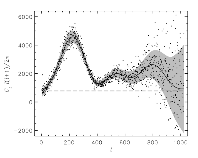
Figure 5: Sample $C_{\ell}$ spectrum recovered from a simulated 90 GHz sky map with MAP-like noise properties. This spectrum can be shown to be an unbiased, nearly minimum variance estimate of the true power spectrum [13].

References

- [1] Smoot, G.F., Bennett, C.L., Kogut, A. et al. (1992) ApJ 396, L1
- [2] Bennett, C.L., Smoot, G.F., Hinshaw, G. et al. (1992) ApJ 396, L7
- [3] Wright, E.L., Meyer, S.S., Bennett, C.L. et al. (1992) ApJ 396, L13
- [4] Bennett, C.L., Banday, A.J., Gorski, K.M. et al. (1996) ApJ 464, L1
- [5] Miller, A.D., Devlin, M.J., Dorwart, W. et al. (1999) ApJ 524, L1
- [6] de Bernardis, P., Ade, P.A.R., Bock, J.J. et al. (2000) Nature 404, 955
- [7] Hanany, S., Ade, P., Balbi, A. et al. (2000) ApJ in press, astro-ph/0005123
- [8] Kogut, A. (1999) in Microwave Foregrounds, eds. de Oliveira-Costa and Tegmark, ASP Conference Series 181, 91
- [9] Press, W.H., Teukolsky, S.A., Vetterling, W.T., & Flannery, B.P. (1992) Numerical Recipes: The Art of Scientific Computing, (2d ed.; Cambridge: Cambridge Univ. Press)
- [10] Wright, E.L., Hinshaw, G., & Bennett, C.L. (1996) ApJ 458, L53
- [11] Muciaccia, P.F., Natoli, P., & Vittorio, N. (1998) ApJ 488, L63
- [12] HEALPix web site: http://www.eso.org/kgorski/healpix/
- [13] Oh, S.P., Spergel, D.N., Hinshaw, G. (1999) ApJ 510, 551