Magnetocentrifugal acceleration of plasma in a nonaxisymmetric magnetosphere

Abstract

Violation of the axial symmetry of a magnetic field essentially modifies the physics of the plasma outflow in the magnetosphere of rotating objects. In comparison to the axisymmetric outflow, two new effects appear: more efficient magnetocentrifugal acceleration of the plasma along particular field lines and generation of MHD waves. Here, we use an ideal MHD approximation to study the dynamics of a cold wind in the nonaxisymmetric magnetosphere. We obtain a self-consistent analytical solution of the problem of cold plasma outflow from a slowly rotating star with a slightly nonaxisymmetric magnetic field using perturbation theory. In the axisymmetric (monopole-like) magnetic field, the first term in the expansion of the terminating energy of the plasma in powers of $\Omega$ is proportional to $\Omega^{4}$, where $\Omega$ is the angular velocity of the central source. Violation of the axial symmetry of the magnetic field crucially changes this dependence. The first correction to the energy of the plasma becomes proportional to $\Omega$. Efficient magnetocentrifugal acceleration occurs along the field lines curved initially in the direction of the rotation. I argue that all the necessary conditions for the efficient magnetocentrifugal acceleration of the plasma exist in the radio pulsar magnetosphere. We calculated the first correction of the rotational losses due to the generation of the MHD waves and analysed the plasma acceleration by these waves.

1 Introduction

The outflow of plasma from rotating magnetised objects is a widespread phenomenon in the Universe. It is observed in a wide range of astrophysical objects of different natures and scales. Some of these objects eject relativistic plasma. The Lorentz factor of plasma ejected by microquasars and AGN is of the order 10 (Mirabel & Rodrigues [1996], Begelman et al. [1984], Pelletier et al. [1996]), although there is evidence that in Blazars the plasma is accelerated to the Lorentz factor $\sim 10^{6}$ (Aharonian et al. [1999]). Radio pulsars also accelerate the plasma to the Lorentz factor $\sim 10^{6}$ (Kennel & Coroniti [1984], Coroniti [1990], Arons [1996]). The problem of the acceleration of the plasma to such high energies remains one of the most important unsolved problems in modern relativistic astrophysics.

The acceleration of plasma can occur in principle due to different dissipative as well as nondissipative processes. Hypothesis have been proposed about the singular behaviour of the relativistic plasma outflow at the “light surface” ([1983]) or at the light cylinder (Mestel & Shibata [1994]) of radio pulsars. These dissipative structures could provide the plasma acceleration. However, recent direct numerical calculations of the relativistic outflows in MHD approximation (Bogovalov [1997]) and force-free approximation (Contpoulos et al. [1999]) have demonstrated that the relativistic plasma flow is actually regular everywhere.

Another mechanism of acceleration due to dissipative processes was proposed by Michel (1982) and Coroniti (1990) in application to radio pulsars. Michel was the first who noticed that the number of charge carriers in the wind from radio pulsars is not enough to sustain the necessary return current in the wind with a striped magnetic field formed at the outflow from the oblique rotator. Coroniti (1990) considered the reconnection process in this magnetic field and came to the conclusion that it can provide the necessary acceleration of the winds from radio pulsars. Up to now this process was considered as the only possible mechanism explaining pulsar wind acceleration. However, recently Luybarskii & Kirk (2000) have revisited the process of wind acceleration due to magnetic field reconnection. They concluded that well before the winds from pulsars such as the Crab pulsar reach high Lorentz factors they will be terminated by the interstellar medium.

A lot of efforts has been spent to obtain the plasma acceleration in frameworks of ideal MHD. There is a general opinion that in all astrophysical objects ejecting plasma, the magnetic field plays an essential role in the dynamics of the plasma. In particular, the magnetic field of a rotating object itself can provide the acceleration of the plasma due to a magnetocentrifugal (below MC) mechanism (Blandford & Payne [1982]). The ideal MHD outflows of plasma in different models and different approximations were investigated in a series of works (Michel [1969], Sulkanen & Lovelace [1990], Ferreira [1997], Vlahakis & Tsinganos [1998], Bogovalov & Tsinganos [1999], Krasnopolsky et al. [1999], Ustyugova et al. [1999]). It follows from these studies that nonrelativistic plasma can be accelerated rather efficiently due to this mechanism. As far as relativistic plasma is concerned, the efficiency of the acceleration of this plasma appears insufficient for astrophysical applications. There were hopes that divergence of the magnetic flux tubes somewhere beyond the light cylinder will result in more efficient acceleration of the plasma due to the pressure gradient of the toroidal magnetic field (Begelman & Li [1994], Takahashi & Shibata [1998]). The only known mechanism for this magnetic flux tube divergence is magnetic self-collimation of the magnetised winds (Heyvaerts & Norman [1989], Chiueh et al. [1991]). This mechanism can, in principle, provide divergence of the field lines at the equatorial plane such that the poloidal field decreases with distance faster than $r^{-2}$. This divergence can take place in the limiting range of distances from the source, since finally the wind expands radially near the equator at $r\rightarrow\infty$ (Heyvaerts & Norman [1989], Chiueh et al. [1991]).

Numerical self-consistent solution of the problem of steady-state plasma outflow in a model with the an initially monopole-like magnetic field shows that collimation really increases the efficiency of nonrelativistic plasma acceleration at the equator (Bogovalov & Tsinganos [1999]). However, collimation of the relativistic plasma outflow appears negligibly small at large Lorentz factors (Bogovalov [1997], Bogovalov [2001]). Therefore, the relativistic plasma is practically not accelerated by the pressure gradient of the toroidal magnetic field. This conclusion is valid not only for the monopole-like model.

The acceleration of the wind due to the pressure gradient of the toroidal magnetic field occurs at the large distances compared to the dimension of the central source (Begelman & Li [1994], Takahashi & Shibata [1998]). The stationary wind from any source is monopole-like at these distances. Therefore, the poloidal magnetic field also becomes monopole-like, since the magnetic field is frozen into the plasma. Thus, the solutions obtained in the monopole-like model actually describe general properties of any axisymmetric wind at large distances from the source.

The application of the monopole-like model is not limited by large distances. This model also gives upper limits on the efficiency of the MC acceleration of the plasma in any other axisymmetric magnetic field (dipolar for example). It is qualitatively clear that the slower the magnetic field decreases with distance, the more efficiently it accelerates the plasma due to a MC mechanism. The monopole-like magnetic field falls down as $r^{-2}$, while the dipolar magnetic field falls down faster than $r^{-2}$. Correspondingly, the plasma is expected to be more efficiently accelerated in the monopole-like magnetic field in compare with the acceleration in the dipolar one. This is why the results obtained in the monopole-like model rule out efficient MC acceleration of the plasma in any other more realistic axisymmetric model. Calculations performed by Contopoulos et al. ([1999]) confirm this conclusion.

Thus, up to now all the attempts to propose an effective mechanism of relativistic plasma acceleration have not been successful. That is why the search for new possible mechanisms to explain relativistic plasma acceleration remains one of the most important problems of relativistic astrophysics.

The disappointing conclusion regarding the low efficiency of the MC acceleration is valid only for axisymmetric magnetic fields, as previous studies considered this process only within the frameworks of axisymmetric models. However, the magnetic field of real astrophysical objects is not axisymmetric. Radio pulsars give us the brightest example of this relation. Therefore, it is important to know how the non axisymmetry of the magnetic field affects the process of MC acceleration. In this paper we try to answer this question.

To clarify the role of the nonaxisymmetry of the magnetic field for the MC acceleration of plasma, a model with the initially monopole-like magnetic field is used in this paper. This model is often used to investigate the processes of plasma collimation and acceleration in the rotating magnetosphere (Michel [1969], Mestel & Selley [1970], Sakurai [1985], Bogovalov [1992], Beskin et al. [1998], Bogovalov & Tsinganos [1999], Tsinganos & Bogovalov [2000]). The word “initially” implies that the magnetic field of the non rotating star looks like the magnetic field of the “magnetic monopole”. This model is very convenient since there are no closed field lines in the flow. It remarkably simplifies the analysis of the plasma acceleration.

The main goal of this paper is to answer the question: how does the nonaxisymmetry of the magnetic field of a star affect the process of plasma acceleration? An attempt to solve the problem of the structure of the magnetosphere of an oblique rotator with a dipole magnetic field in mass-less approximation has been done by Beskin et al. ([1983]). The first step in the solution of this problem in the MHD approximation has been done in the work of Bogovalov ([1999]). In this work, the problem of plasma flow in the magnetosphere of the oblique rotator with an initially split-monopole magnetic field was solved. The modulus of the magnetic field was axisymmetric and only the direction of the magnetic field varied with time and the azimuthal angle. It was found that the acceleration remains non efficient in this flow as well. In the present paper, we are interested in the affect of the nonaxisymmetry of the modulus of the magnetic field on the process of plasma acceleration.

Plasma flow is described by a system of non linear equations in partial derivatives. Usually these equations can be integrated only numerically. There is one exception from this rule. Sometimes the problem can be solved self-consistently and analytically if we are interested in small corrections to the known solution. These corrections can arise if the known flow is perturbed slightly by additional small forces. In particular, slow rotation can be considered as a small perturbation of some known flow from the non rotating star. This approach was firstly successfully applied for the numerical self-consistent solution of the flow of the solar wind by Nurney and Suess ([1975]). Later Bogovalov ([1992]) has used this approach for the fully analytical, self-consistent solution of the problem of the cold plasma outflow, relativistic as well as nonrelativistic, from a slowly rotating star. In recent years, this method has also been used to solve a range of problems by Beskin (see Beskin & Okamoto [2000]) and references therein). The idea of the present work is the following: if the nonaxisymmmetry of the magnetic field modifies the process of MC acceleration of the plasma, this modification can be seen at the level of the slow rotation of the object. Therefore, to answer the question: does the nonaxisymmetry of the magnetic field modify the process of acceleration of the plasma, we investigate the acceleration of plasma in the nonaxisymmetric magnetic field at slow rotation.

This paper is organised as follows. In Sect. 2 we present ideal MHD equations defining the dynamics of cold relativistic plasma. A self-consistent analytical solution of the problem is given in Sec. 3. The solution in the wave zone is given in Sect. 4. The possible astrophysical implications of the results are discussed in Sec. 5.

2 Basic equations and relationships

The system of time dependent equations defining the temporal evolution of the relativistic plasma outflow in an ideal MHD approximation is as follows (Akhiezer et al. [1975]):

$$mn({\partial\gamma{\bf v}\over\partial t}+({\bf v\nabla})\gamma{\bf v})=q\cdot{\bf E}+{1\over c}~{}{\bf j}\times{\bf H},$$ (1)

$${\partial{\bf H}\over c\partial t}=-curl~{}{\bf E},$$ (2)

$$curl~{}{\bf H}={4\pi\over c}{\bf j}+{\partial{\bf E}\over c\partial t},$$ (3)

$$div~{}{\bf H}=0,$$ (4)

$$div~{}{\bf E}=4\pi q,$$ (5)

$${\partial n\over\partial t}+div({\bf v}n)=0.$$ (6)

$${\bf E}+{1\over c}{\bf v}\times{\bf H}=0.$$ (7)

Gravitation is neglected in these equations. It is convenient to consider the plasma flow in a spherical coordinate system. In this system, the equations of motion are

$$mn({\partial\gamma v_{r}\over\partial t}+({\bf v\nabla})\gamma v_{r}-{\gamma(v_{\theta}^{2}+v_{\varphi}^{2})\over r})=$$ (8)

$$q\cdot E_{r}+{1\over 4\pi}\Bigl{\{}({1\over r\sin{\theta}}{\partial H_{r}\over\partial\varphi}-{1\over r}{\partial(rH_{\varphi})\over\partial r})H_{\varphi}-$$

$$-({\partial(rH_{\theta})\over r\partial r}-{\partial H_{r}\over r\partial\theta})H_{\theta}+{1\over c}(H_{\theta}{\partial E_{\varphi}\over\partial t}-H_{\varphi}{\partial E_{\theta}\over\partial t})\Bigr{\}},$$

$$mn({\partial\gamma v_{\theta}\over\partial t}+({\bf v\nabla})\gamma v_{\theta}+{\gamma(v_{r}v_{\theta}-v_{\varphi}^{2}\cot\theta)\over r})=$$ (9)

$$q\cdot E_{\theta}+{1\over 4\pi}\Bigl{\{}({\partial(rH_{\theta})\over r\partial r}-{\partial H_{r}\over r\partial\theta})H_{r}-$$

$$-{H_{\varphi}\over r\sin\theta}({\partial\sin\theta H_{\varphi}\over\partial\theta}-{\partial H_{\theta}\over\partial\varphi})+$$

$$+{1\over c}(H_{\varphi}{\partial E_{r}\over\partial t}-H_{r}{\partial E_{\varphi}\over\partial t})\Bigr{\}},$$

$$mn({\partial\gamma v_{\varphi}\over\partial t}+({\bf v\nabla})\gamma v_{\varphi}+{\gamma(v_{r}v_{\varphi}+v_{\theta}v_{\varphi}\cot\theta)\over r})=$$ (10)

$$q\cdot E_{\varphi}+{1\over 4\pi}\Bigl{\{}{1\over r\sin\theta}({\partial\sin\theta H_{\varphi}\over\partial\theta}-{\partial H_{\theta}\over\partial\varphi})H_{\theta}-$$

$$-({1\over r\sin\theta}{\partial H_{r}\over\partial\varphi}-{\partial rH_{\varphi}\over r\partial r})H_{r}+$$

$$+{1\over c}(H_{r}{\partial E_{\theta}\over\partial t}-H_{\theta}{\partial E_{r}\over\partial t})\Bigr{\}},$$

and the induction equations:

$${\partial H_{r}\over c\partial t}=-{1\over r\sin\theta}({\partial(\sin\theta E_{\varphi})\over r\partial\theta}-{\partial E_{\theta}\over\partial\varphi}),$$ (11)

$${\partial H_{\theta}\over c\partial t}=-({1\over r\sin\theta}{\partial E_{r}\over r\partial\varphi}-{\partial(rE_{\varphi})\over r\partial r}),$$ (12)

$${\partial H_{\varphi}\over c\partial t}=-({\partial(rE_{\theta})\over r\partial r}-{\partial E_{r}\over r\partial\theta}).$$ (13)

The laws of conservation of the magnetic field and the matter flux, together with the Coulomb law, take the following form:

$${1\over r^{2}}{\partial(r^{2}H_{r})\over\partial r}+{1\over r\sin\theta}{\partial\sin\theta H_{\theta}\over\partial\theta}+{1\over r\sin\theta}{\partial H_{\varphi}\over\partial\varphi}=0.$$ (14)

$${\partial n\over\partial t}+{1\over r^{2}}{\partial(r^{2}nv_{r})\over\partial r}+{1\over r\sin\theta}{\partial\sin\theta nv_{\theta}\over\partial\theta}+{1\over r\sin\theta}{\partial nv_{\varphi}\over\partial\varphi}=0.$$ (15)

$${1\over r^{2}}{\partial(r^{2}E_{r})\over\partial r}+{1\over r\sin\theta}{\partial\sin\theta E_{\theta}\over\partial\theta}+{1\over r\sin\theta}{\partial E_{\varphi}\over\partial\varphi}=4\pi q.$$ (16)

The ideal MHD conditions are

$$E_{r}+{1\over c}(v_{\theta}H_{\varphi}-v_{\varphi}H_{\theta})=0,$$ (17)

$$E_{\theta}+{1\over c}(v_{\varphi}H_{r}-v_{r}H_{\varphi})=0,$$ (18)

$$E_{\varphi}+{1\over c}(v_{r}H_{\theta}-v_{\theta}H_{r})=0.$$ (19)

In this system, $q$ is the induced space electric charge density, $\theta$ is the polar angle and $\varphi$ is the azimuthal angle.

The electric field in the axisymmetrically rotating steady state magnetosphere is connected with the poloidal magnetic field as follows: ${\bf E}=r\sin\theta\Omega/c{\bf B_{p}\times e_{\varphi}}$ and $E_{\varphi}=0$ (Weber & Davis [1967]). For the nonaxisymmetric magnetic field the same relationship is also valid, provided that the flow is in the steady state and all the variables vary periodically with time (Beskin et al. [1983]). In the spherical coordinates, the relationships take the form

$$E_{\theta}=-{r\sin\theta\Omega\over c}H_{r},~{}~{}E_{r}={r\sin\theta\Omega\over c}H_{\theta},~{}~{}E_{\varphi}=0.$$ (20)

It is easy to show that these relationships indeed satisfy all the equations of the electric field in a rotating magnetosphere. At stationary rotation, all the variables depend on $\varphi$ and $t$ in the spherical system of coordinates as the difference $\xi=\varphi-\Omega t$. Then, the induction equation (11) is reduced to the equation

$${\partial\over\partial\xi}({E_{\theta}\over r\sin\theta}+{\Omega H_{r}\over c})=0$$ (21)

which is fulfilled due to Eq. (20). The same is valid for the induction equation (12) which is reduced to the equation

$${\partial\over\partial\xi}({E_{r}\over r\sin\theta}-{\Omega H_{\theta}\over c})=0.$$ (22)

The third induction equation (13) after the substitution of Eqs. (20) is reduced to the magnetic flux conservation condition (14). Eq. (20) also satisfies the boundary conditions on the surface of the star where the tangential components of the electric field should be continuous. It follows from the ideal MHD conditions (17-19) that below the surface of the star the tangential components of the electric field are $E_{\varphi}=0$ and $E_{\theta}=-\Omega r\sin\theta/cH_{r}$. They exactly equal the tangential components of the electric field directly above the star surface, given by (20).

3 Acceleration of the plasma at slow rotation

3.1 Acceleration in the axisymmetric magnetic field

The solution of the problem of steady state plasma outflow can be expanded in powers of $\Omega$. The poloidal magnetic field, the plasma density, the poloidal velocity and the Lorentz factor of the plasma are invariant in relation to the rotation direction at the axisymmetric outflow. Therefore they are expanded in even powers of $\Omega$. Correspondingly, the toroidal magnetic field and the toroidal velocity are expanded in odd powers of $\Omega$, since these variables change sign at the change of the direction of rotation. Therefore, the expansion of the solution in the powers of $\Omega$ takes the form

$${\bf H}_{p}={\bf H}_{p,0}+\Omega^{2}{\bf H}_{p,2}+....,$$ (23)

$$H_{\varphi}=\Omega H_{\varphi,1}+\Omega^{3}H_{\varphi,3}+....,$$ (24)

$${\bf v}_{p}={\bf v}_{p,0}+\Omega^{2}{\bf v}_{p,2}+....,$$ (25)

$$v_{\varphi}=\Omega v_{\varphi,1}+\Omega^{3}v_{\varphi,3}+....,$$ (26)

$$n=n_{0}+\Omega^{2}n_{2}+....,$$ (27)

$$\gamma=\gamma_{0}+\Omega^{2}\gamma_{2}+\Omega^{4}\gamma_{4}+......,$$ (28)

where lower index “0” denotes the variables for the nonrotating star. The first corrections to the unperturbed cold plasma outflow from the nonrotating star arising at slow rotations of the star with a monopole-like magnetic field were calculated analytically by Bogovalov ([1992]). The first order corrections to the toroidal magnetic field and the toroidal velocity are as follows

$$H_{\varphi,1}=-H_{p,0}{r\sin\theta\over v_{0}},~{}~{}~{}~{}v_{\varphi,1}=0,$$ (29)

where

$$H_{p,0}=H_{*}({R_{*}\over r})^{2}$$ (30)

is the monopole-like magnetic field of the star and the lower index “*” denotes the values on the surface of the star. It follows from (29) that the first correction to the energy of the plasma accelerated in the monopole-like magnetic field is proportional to $\Omega^{4}$. Indeed, the equation for the Lorentz factor of the plasma has the form (Landau & Lifshitz [1975])

$$mnc^{2}({\partial\gamma\over\partial t}+({\bf v\nabla})\gamma)={\bf jE}.$$ (31)

The second order correction to the Lorentz factor is defined as follows

$$mn_{0}c^{2}v_{0}\Omega^{2}{\partial\over r}\gamma_{2}={r\Omega\sin\theta\over 4\pi}H_{p,0}{\partial\over r\partial r}(rH_{\varphi,1}).$$ (32)

But according to (29) and (30) the right hand part of this equation is equal to zero. Thus, $\gamma_{2}=0$. The fact that the first correction to the Lorentz factor at the axisymmetrical outflow begins with the term proportional to $\Omega^{4}$ reflects the very low efficiency of the MC acceleration in the monopole-like magnetic field.

3.2 Acceleration in the nonaxisymmetric magnetic field

The Lorentz factor of the plasma accelerated in the nonaxisymmetric magnetic field is already not invariant in relation to the direction of the rotation. In this case it can (but not must) depend on the sign of $\Omega$. The expansion of the Lorentz factor in $\Omega$ takes the general form

$$\gamma=\gamma_{0}+\Omega\gamma_{1}+\Omega^{2}\gamma_{2}+\Omega^{3}\gamma_{3}+...$$ (33)

In the axisymmetric case, $\gamma_{1}=\gamma_{3}=0$ (generally speaking, the term $\gamma_{2}=0$ applies only for the monopole-like magnetic field). In the nonaxisymmetric case these terms can (but not must) differ from zero. If for example $\gamma_{1}\neq 0$, it would imply that the acceleration of the plasma in the nonaxisymmetric magnetic field is essentially more efficient in comparison to the acceleration in the axisymmetric magnetic field, at least for the case of slow rotation. To make sure that indeed $\gamma_{1}\neq 0$, it is sufficient to do this for the magnetic field having small nonaxisymmetry. In this case, the problem can be solved analytically.

3.3 Outflow at $\Omega=0$ in the slightly nonaxisymmetric magnetic field

Let us initially consider the cold plasma outflow from the nonrotating star with a slightly nonaxisymmetric magnetic field. It follows from (31) that the energy of the cold plasma is constant since the electric field ${\bf E}=0$ everywhere. For the slightly nonaxisymmetric magnetic field the solution also can be expanded on a small parameter, $\varepsilon$, characterising the nonaxisymmetry of the initial split-monopole magnetic field. This expansion has the form

$${\bf H}_{p}={\bf H}_{p,0}+\varepsilon{\bf h}_{p,1}+....,$$ (34)

$$H_{\varphi}=\varepsilon h_{\varphi,1}+\varepsilon^{2}h_{\varphi,2}+...$$ (35)

$${\bf v}_{p}={\bf v}_{p,0}+\varepsilon{\bf V}_{p,1}+\varepsilon^{2}{\bf V}_{p,2}+....,$$ (36)

$$v_{\varphi}=\varepsilon V_{\varphi,1}+\varepsilon^{2}V_{\varphi,2}+....,$$ (37)

$$n=n_{0}+\varepsilon\tilde{n}_{1}+....,$$ (38)

but

$$\gamma=\gamma_{0},$$ (39)

since the energy of the cold plasma is constant. It is convenient to consider the perturbation of the magnetosphere due to a non uniform distribution of the magnetic field on the stellar surface. We assume for simplicity that the magnetic field has its own axis of symmetry ${\bf m}$ not coinciding with the axis of rotation, as is shown in Fig. 1. It is convenient firstly to solve the problem in the coordinate system where the magnetic field is axially symmetric and then to transform the solution to the laboratory coordinate system. The equation for the first corrections in the system where the magnetic field is axisymmetric follows from Eq. (9) and takes the form

$$mn_{0}\gamma_{0}v_{0}{\partial rV_{\chi,1}\over r\partial r}={H_{0}\over 4\pi}({\partial rh_{\chi,1}\over r\partial r}-{\partial h_{r,1}\over r\partial\chi}),$$ (40)

where $\chi$ is the polar angle in the system of the symmetry of the flow. It is convenient to introduce the flux function $\psi$. The components of the poloidal magnetic field can be expressed through the flux function as follows

$$H_{\chi}=-{1\over r\sin\chi}{\partial\psi\over\partial r};~{}~{}~{}H_{r}={1\over r\sin\chi}{\partial\psi\over r\partial\chi}.$$ (41)

The expansion of the function $\psi$ in powers of $\varepsilon$ is

$$\psi=H_{*}R^{2}_{*}(1-\cos\chi+\varepsilon f({\bf r})+....).$$ (42)

Taking into account that due to the ideal MHD condition ${\bf v}=v{\bf H}/H$, it is easy to obtain the equation for $f$ (Bogovalov [1992])

$$f_{rr}+{2\over r}f_{r}=({R_{a}\over r})^{2}(f_{rr}+{(1-\eta^{2})\over r^{2}}{\partial^{2}f\over\partial^{2}\eta}),$$ (43)

where $\eta=\cos\chi$, $R_{a}=\sqrt{H_{*}^{2}R_{*}^{2}/4\pi mn_{*}\gamma_{0}v_{0}^{2}}$ is the Alfven (or fast magnetosonic) radius of the unperturbed flow. The perturbation $f$ can be presented as

$$f=\sum_{m}f_{m}(r)Q_{m}(\eta),$$ (44)

where $Q_{m}$ are the eigenfunctions of the differential equation $(1-\eta^{2})\partial^{2}f/\partial^{2}\eta Q_{m}=-m(m+1)Q_{m}$. They have the form $Q_{m}(\eta)=(1-\eta^{2})\partial P_{m}(\eta)/\partial\eta$, where $P_{m}$ are the Legendre polynomials of the order m.

The equation for $f_{m}$ takes the form

$$(x^{2}-1){d^{2}f_{m}\over d^{2}x}+2x{df_{m}\over dx}+{m(m+1)\over x^{2}}f_{m}=0,$$ (45)

where $x=r/R_{a}$. The general solution can be presented as a sum $f_{m}=a_{m}Z_{m}(x)+b_{m}Y_{m}(x)$ of two independent solutions. One of them, $Z_{m}$, is regular at the point $x=1$ and another, $Y_{m}$, is singular at this point. The condition of regularity of the solution at this point gives $b_{m}=0$. The regular solution of Eq. (45) is $Z_{m}(x)=P_{m}(1/x)$. Therefore, the general solution of the problem regular at the Alfven surface can be presented as follows

$$f=\sum_{m}a_{m}P_{m}(1/x)Q_{m}(\eta).$$ (46)

The boundary conditions on the stellar surface define the numerical coefficients $a_{m}$.

It is convenient to take one term from expansion (46) which corresponds to the simplest non uniformity of the magnetic field on the stellar surface. It is especially interesting to consider the non uniformity which increases the magnetic field at the magnetic poles and decreases the magnetic field at the magnetic equator. The term with $m=2$ corresponds to this distribution. The correction to the solution in this case is

$$f={(3/x^{2}-1)\over(3/x^{2}_{*}-1)}\sin^{2}\chi\cos\chi.$$ (47)

The corrections to the magnetic field are

$$h_{\chi,1}={6H_{*}R_{*}^{2}\over R_{a}^{2}x^{4}(3/x_{*}^{2}-1)}\sin\chi\cos\chi,$$ (48)

$$h_{r,1}={(3/x^{2}-1)H_{*}R_{*}^{2}\over r^{2}(3/x_{*}^{2}-1)}(2\cos^{2}\chi-\sin^{2}\chi).$$ (49)

It is seen that the radial perturbation of the magnetic field is positive at the magnetic poles and negative at the equator (at $\varepsilon>0$). It is interesting that the perturbation of the radial component of the magnetic field decreases as $r^{-2}$ at $r\rightarrow\infty$ . The initial magnetic field has the same dependence. This means that the flow is not spherically symmetric at $r\rightarrow\infty$. This is one of the features of supersonic flows. The magnetic forces decrease with distance so fast that the supersonic plasma moves ballistically along straight lines defined by the initial conditions. The magnetic pressure gradient across the flow lines is not able to change the trajectories of the particles of the plasma to restore the spherical symmetry at $r\rightarrow\infty$.

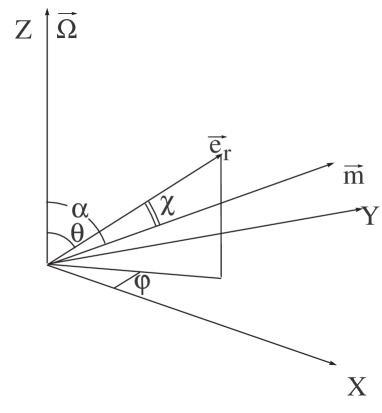
Figure 1: The geometry of the coordinate systems connected with the axis of rotation (axis ${\bf\Omega}$) and the axis of symmetry of the magnetic field (axis ${\bf m}$) inclined to the rotation axis ${\bf\Omega}$ under the angle $\alpha$. ${\bf e}_{r}$ is the unit vector directed along ${\bf r}$.

The components of the arbitrary vector $\bf A$ in the spherical coordinate system with the polar axis directed along the symmetry axis of the magnetic field ${\bf m}$ (dashed coordinate system) can be transformed into the components of the same vector in the laboratory coordinate system, shown in Fig. 1 as follows:

$$A_{r}=A_{r}^{{}^{\prime}},$$

$$A_{\theta}={A_{\chi}^{{}^{\prime}}(\cos\alpha\sin\theta-\sin\alpha\cos\theta\cos\varphi)-A_{\varphi}^{{}^{\prime}}\sin\varphi\sin\alpha\over\sin\chi},$$

$$A_{\varphi}={A_{\varphi}^{{}^{\prime}}(\cos\alpha\sin\theta-\sin\alpha\cos\theta\cos\varphi)+A_{\chi}^{{}^{\prime}}\sin\varphi\sin\alpha\over\sin\chi},$$

where $\alpha$ is the inclination angle of the magnetic axis in relation to the axis $\bf\Omega$. The equation connecting the coordinates in the systems is as follows

$$\cos\chi=\sin\alpha\sin\theta\cos\varphi+\cos\alpha\cos\theta.$$ (50)

The transformation of the vector ${\bf A}$ with $A_{\varphi}=0$ at $\alpha=\pi/2$ (orthogonal rotator) is of special interest for us below. The components of the vector are connected as follows in this case

$$A_{\theta}=-A_{\chi}^{{}^{\prime}}{\cos\theta\cos\varphi\over\sqrt{1-\sin^{2}\theta\cos^{2}\varphi}}$$ (51)

and

$$A_{\varphi}=A_{\chi}^{{}^{\prime}}{\sin\varphi\over\sqrt{1-\sin^{2}\theta\cos^{2}\varphi}}.$$ (52)

3.4 Plasma acceleration in the slightly nonaxisymmetric magnetic field at slow rotation

At slow rotation and small nonaxisymmetry of the magnetic field the solution can be expanded in two parameters: $\Omega$ and $\varepsilon$. The expansion takes a form

$${\bf H}_{p}={\bf H}_{p,0}+\varepsilon{\bf h}_{p,1}+....,$$ (53)

$$H_{\varphi}=\Omega H_{\varphi,1}+\varepsilon h_{\varphi,1}+....,$$ (54)

$${\bf v}_{p}={\bf v}_{p,0}+\varepsilon{\bf V}_{p,2}+....,$$ (55)

$$v_{\varphi}=\varepsilon V_{\varphi,3}+....,$$ (56)

$$n=n_{0}+\varepsilon n_{1}+....,$$ (57)

$$\gamma=\gamma_{0}+\varepsilon\Omega\delta\gamma+.......$$ (58)

It follows from (31) that $\delta\gamma$ satisfies the equation

$$mn_{0}c^{2}\Omega\varepsilon v_{0}{\partial\delta\gamma\over\partial r}=E_{\theta}j_{\theta},$$ (59)

where

$$j_{\theta}=\varepsilon{c\over 4\pi}({1\over r\sin\theta}{\partial h_{r,1}\over\partial\varphi}-{\partial\over r\partial r}rh_{\varphi,1}),$$ (60)

and $E_{\theta}$ is defined by Eq. (20). Let us calculate $\delta\gamma$ for the particular case of orthogonal rotation ($\alpha=\pi/2$) for the flow in the equatorial plane ($\theta=\pi/2$). The transformation of the solution (51, 52) to the laboratory coordinate system gives

$$j_{\theta}={c\over 4\pi}{6\varepsilon H_{*}R_{*}^{2}\sin\xi\cos\xi\over r^{3}(3/x_{*}^{2}-1)}.$$ (61)

Integration of Eq. (59) with Eq. (61) gives

$$\gamma=\gamma_{0}-\gamma_{0}{\Omega R_{*}\over c}{v_{0}\over c}{6\varepsilon\sin\xi\cos\xi\over(3-x^{2}_{*})},$$ (62)

where

$$\xi=\varphi-\Omega t.$$ (63)

It is seen that the violation of axial symmetry of the magnetic field essentially modifies the acceleration process. The first correction to the Lorentz factor of the plasma is proportional to $\Omega^{4}$ in the axisymmetric magnetic field, while even the small nonaxisymmetry of the magnetic field makes the dependence much stronger. The first correction to the Lorentz factor begins with the term proportional to $\Omega$.

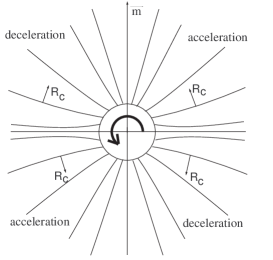
Figure 2: Outflow in the magnetic field of a star with a monopole-like magnetic field having small non uniformity on the surface of the star. The magnetic field is slightly stronger at the poles and slightly weaker at the magnetic equator. The magnetic field is axially symmetric in relation to the axis $\bf m$. The particular case when the axis of the symmetry of the magnetic field is perpendicular to the axis of rotation (orthogonal rotator) is presented. At a slow rotation, the acceleration of plasma occurs along the field lines which curve with a radius $R_{c}$ directed into the direction of rotation shown by thick arrow.

The schematic structure of the field lines unperturbed by the rotation is shown in Fig. 2. The view from the top is presented. The acceleration of the plasma takes place in the sectors where $\sin\varphi\cos\varphi<0$ (at $t=0$, $\varphi=0$ at the direction along ${\bf m}$). In other sectors the plasma is decelerated. It follows from the figure that the plasma is accelerated where the field lines unperturbed by the rotation are curved into the direction of the rotation and is decelerated where they are curved in the opposite direction. This behaviour of the plasma has a simple mechanical analogy.

The motion of the magnetised plasma can be considered in some sense as a motion of a bead on a wire (Blandford & Payne [1982]). The bead is accelerated centrifugally during the motion along the wire, provided that the wire is not in the shape of an Archimedian spiral with the components $dl_{\varphi}$ and $dl_{r}$ defined by the equation

$${dl_{\varphi}\over dl_{r}}=-{r\Omega\sin\theta\over v_{r}}.$$

It is easy to demonstrate that any departure of the wire shape from the Archimedian spiral results in variation of the energy of the bead. The bead will be accelerated centrifugally under the condition $|{dl_{\varphi}\over dl_{r}}|<|{r\Omega\sin\theta\over v_{r}}|$ and decelerated in the opposite case. The plasma behaves exactly in accordance with this mechanical model. It follows from (29) that the field lines of the axisymmetric magnetic field form the Archimedian spiral at small $\Omega$. At the nonaxisymmetric outflow, the toroidal magnetic field is a linear superposition of perturbations from rotation and the nonaxisymmetry. The initial nonaxisymmetry straightens the magnetic field lines in the sectors where $\sin\varphi\cos\varphi<0$. The shape of the field lines here satisfies the inequality $|{dl_{\varphi}\over dl_{r}}|<|{r\Omega\sin\theta\over v_{r}}|$. The plasma is accelerated in this case. In other sectors, the field lines are curved in an azimuthal direction more strongly in comparison to the Archimedian spiral. Therefore, the plasma is decelerated.

4 Generation of magneto sound waves

The modification of the MC acceleration is not the only new feature of the outflows in the magnetic field with violated axial symmetry. The source with the nonaxisymmetric magnetic field excites the magnetohydrodynamical (but not magnetodipole) waves in the wind. Perturbation theory allows us to investigate this process while the amplitude of these waves is small.

In the axisymmyteric case, the azimuthal magnetic field generated by the rotation is defined by Eq.(29). Perturbation theory can be applied while the pressure of the toroidal magnetic field in the co-moving coordinate system is less than the pressure of the unperturbed poloidal magnetic field (Bogovalov [1997]). In the laboratory coordinate system this condition takes the form

$$H_{\varphi}^{2}-E^{2}<H_{p}^{2},$$ (64)

This inequality limits the application of the perturbation theory by the distances $r$ less than $\gamma_{0}v_{0}/\Omega$. When the last value becomes less than $R_{a}$, the perturbation becomes strong everywhere in the flow. Thus, the perturbation theory can be applied only if

$${\Omega R_{a}\over\gamma_{0}v_{0}}<1.$$ (65)

The objects satisfying condition (65) are referred to as slow rotators. In the opposite case they are fast rotators. Analysis shows that all radio pulsars, including the Crab pulsar, are slow rotators at the conventional parameters of the winds (Bogovalov [1999]).

Eq. (65) defines the condition under which the perturbation of the flow in the subsonic region remains small compared with the initial magnetic field. Our use of the perturbation theory is valid given an additional restriction. During the calculation of the first corrections, we neglected the contribution of the energy density of the toroidal and electric fields generated by the rotation into the inertial mass of the plasma. In order words, it was assumed that the condition

$$mc^{2}n^{{}^{\prime}}\gg{H^{{}^{\prime}2}_{\varphi}\over 4\pi}$$ (66)

is fulfilled, where the upper index “${}^{{}^{\prime}}$” denotes values in the co-moving coordinate frame. It results in the additional condition

$$R_{a}\ll R_{L},$$ (67)

where $R_{L}=\Omega/c$ is the radius of the light cylinder. Thus, our consideration is valid under the conditions (65) and (67) in the region limited by the radius $\gamma_{0}v_{0}/\Omega$.

The objects with weak violation of the axial symmetry excite small amplitude MHD waves in the outflowing wind, which can be considered in the framework of the perturbation theory. These waves are formed in the wave zone with dimensions of the wavelength $\lambda=V_{w}/\Omega$ (Landau & Lifshitz [1986]), where $V_{w}$ is the velocity of the wave propagating in the moving plasma. The fast magnetosonic velocity of the cold wind decreases with an increase in $r$. In the region $r>R_{a}$, the fast magnetosonic velocity of the plasma $v_{f}$ is small compared with $v_{0}$ for slow rotators and the condition $v_{0}\gg v_{f}$ is fulfilled everywhere along the flow, under condition (67). The wavelength can be estimated as $\lambda\approx v_{0}/\Omega$ in this region. Thus, four scales appear in the problem. One is the initial radius of the Alfven (or fast magnetosonic) surface, $R_{a}$. Others are the radius of the wave zone $\lambda$, the radius of the light cylinder $R_{L}$ and the radius $r_{max}=\gamma_{0}\lambda$, where the perturbation theory itself can not be applied. The inequality $R_{a}/\gamma_{0}\lambda<1$ is fulfilled for the slow rotators. For the nonrelativistic plasma, $r_{max}=\lambda$. The wave zone is located in the region where perturbation theory can not be applied. Therefore, the generation of MHD waves in the nonrelativistic winds cannot be considered in the framework of the perturbation theory developed here. However, in the relativistic plasma with $\gamma_{0}\gg 1$ there is a gap between $\lambda$ and $\gamma_{0}\lambda$ where the perturbation theory remains valid. The MHD wave generation can be considered in the framework of this theory.

It is easy to extend our solution to the zone $\lambda<r<\gamma_{0}\lambda$, following Landau & Lifshitz ([1986], sect. 74). The electric and magnetic fields in the outgoing wave depend on $r$ and $t$ as $A_{i}(t-r/v_{0})/r$, where $A_{i}$ are unknown functions. In the zone $R_{*}\ll r<\lambda$ the solution has a form $B_{i}(t)/r$. Both solutions must coincide at $r=\lambda$. This implies that $A_{i}=B_{i}(t-r/v_{0})$. So, we need only to define functions $B_{i}$ of the solution obtained in the zone $r<\lambda$ to obtain the solution at $r>\lambda$.

It was pointed out that the perturbation of the radial component of the magnetic field $h_{r}$, proportional to $\varepsilon$, falls down as $r^{-2}$ at large $r$. This perturbation results in the perturbation of the toroidal magnetic field (see Eq. (29))

$$h_{\varphi}=-{\Omega r\sin\theta\over v_{0}}h_{r}$$ (68)

and in the perturbation of the $\theta$ component of the electric field (see Eq. (20))

$$e_{\theta}=-{\Omega r\sin\theta\over c}h_{r}.$$ (69)

The electric and magnetic fields from (68) and (69) decrease with distance as $r^{-1}$ at $r\gg R_{*}$, since $h_{r}$ has the following dependence ( see Eq. (49))

$$h_{r}=-\varepsilon{H_{*}R^{2}_{*}\over r^{2}(3/x_{*}^{2}-1)}(3\cos^{2}\chi-1).$$ (70)

All other terms in Eq. (49) are neglected since they decrease with $r$ faster than $r^{-2}$. According to Eq. (50) and Eq. (63), $\cos\chi$ depends on $t$ and $\varphi$ in the combination $\xi=\varphi-\Omega t$. To obtain the solution at $r>\lambda$, we have to replace it by the combination $\varphi-\Omega(t-t/v_{0})$. As a result, $\cos\chi$ takes the form (see Eq. (50))

$$\cos\chi=\sin\alpha\sin\theta\cos(\varphi-\Omega(t-r/v_{0}))+\cos\alpha\cos\theta.$$ (71)

The solution (68,69,70,71) allows us to define a correction to the rotational losses of the central object due to the emission of the MHD waves in the wind and to estimate the effect of the wind acceleration by these waves. The correction to the $r$ component of the Poynting flux ${\bf S}={c\over 4\pi}E\times H$ due to the perturbation of the electric and magnetic fields is as follows

$$S_{r}=-\varepsilon v_{0}{H_{*}^{2}R_{*}^{2}\over 2\pi r^{2}(3/x_{*}^{2}-1)}({\Omega R_{*}\sin\theta\over v_{0}})^{2}(3\cos^{2}\chi-1).$$ (72)

The ratio of this correction over the particle flux density in $mc^{2}$ units is as follows

$$\delta\sigma=-2\varepsilon({\Omega R_{a}\sin\theta\over c})^{2}\gamma_{0}{(3\cos^{2}\chi-1)\over(3/x_{*}^{2}-1)}.$$ (73)

This value shows the maximal possible variation of the Lorentz factor of the plasma at the full absorption of the MHD wave.

Integration of the correction to the Poynting flux over a surface surrounding the source gives the first correction to the rotational losses of the central object,

$$\delta\dot{E}_{rot}={4\over 15}\varepsilon\Omega^{2}{(H_{*}R_{*}^{2})^{2}\over v_{0}(3/x_{*}^{2}-1)}(3\cos^{2}\alpha-1).$$ (74)

The zero order expression for the rotational losses is given in (Bogovalov [1999]). As was expected, the departure from uniform distribution of the magnetic field lines on the surface of the star changes the rotational losses. Correction (74) depends on the sign of $\varepsilon$ and does not go to zero even at axisymmetric rotation ($\alpha=0$). This fact has a simple explanation. The total Poynting flux from an axisymmetrically rotating object depends on the distribution of the poloidal magnetic field on latitude at a large distance from the source (Bogovalov [1999]). At the fixed total magnetic flux, the rotational losses increase when the magnetic flux is more concentrated at the equator. The concentration of the magnetic flux at the poles consequently results in the decrease of rotational loss. Eq. (74) describes this dependence. The magnetic flux is concentrated at the poles for $\varepsilon>0$ on the surface of the star, but according to (49), at large distances the magnetic flux is more concentrated at the equator. Therefore, the rotational losses increase for $\varepsilon>0$ and decrease in the opposite case.

Qualitatively, this also explains the fact that according to Eq. (74) the rotational losses decrease at the orthogonal rotation (at $\varepsilon>0$). In this case, the magnetic flux at large distances is more concentrated along the plane of the magnetic equator, oriented perpendicular to the rotational equator. The average magnetic field in the equatorial plane decreases and results in the decrease in rotational losses.

The MHD wave propagating in the wind changes the energy of the particles of the plasma. The variation in the energy is described by Eq. (31) with the electric current ${\bf j}={c\over 4\pi}(curl{\bf H}-{1\over c}{\partial{\bf E}\over\partial t})$. Substitution of solutions (68, 69) in this expression gives

$$j_{\theta}={c\over 4\pi}{\Omega^{2}r\sin\theta\over v_{0}^{2}\gamma_{0}^{2}}{\partial h_{r}\over\partial\xi}.$$ (75)

The correction to the Lorentz factor of the plasma depends on its arguments, as $\delta\gamma(r,\xi)$. After substitution of this expression and (75) in Eq. (31), we obtain

$${\partial\delta\gamma\over\partial r}=-6\varepsilon R_{a}^{2}{\Omega^{3}\sin^{3}\theta\over\gamma_{0}v_{0}c^{2}}{\cos\chi\sin\alpha\sin\xi\over(3/x_{*}-1)}.$$ (76)

Formally, integration of Eq. (76) over $r$ gives an infinite result. It is clear why this should occur. We do not take into account the decrease in the amplitude of the MHD wave due to the redistribution of energy between waves and particles of the plasma. However, we can estimate the variation in the energy of the plasma depending on $r$. Integration of Eq. (76) gives

$$\delta\gamma=-6\varepsilon({R_{a}\Omega\sin\theta\over c})^{2}{\sin\theta\cos\chi\sin\alpha\sin\xi\over(3/x_{*}^{2}-1)}{r\Omega\over\gamma_{0}v_{0}}.$$ (77)

The lower limit of integration is neglected here. This correction can be negative or positive, depending on the sign of $\cos\chi\sin\xi$. Thus, we consider the process of redistribution of energy, but not pure acceleration. Comparison of Eq. (77) with Eq. (73) shows that even at the distance $\gamma_{0}\lambda$ only a small part of the energy of the wave is transformed into the energy of the plasma and vice versa at $\gamma_{0}\gg 1$. So, this process is extremely noneffective in the relativistic regime.

5 Implications for the physics of relativistic winds from radio pulsars

It is generally believed that $e^{\pm}$ plasma is produced and initially accelerated in the pulsar magnetosphere in the so-called electrostatic gaps (Ruderman & Sutherland [1975], Arons [1981], Cheng et al. [1986], Romani [1996]). The ideal MHD does not apply to these gaps. However, these gaps occupy only a small part of the magnetosphere. They produce the initially relativistic plasma, which is dense enough to screen the electric field and to provide the ideal MHD conditions outside the gaps. Therefore, the flow of this plasma can be described in an ideal MHD approximation as the wind. Below, we assume for simplicity that the wind with a prescribed initial density and Lorentz factor is formed somewhere near the surface of the pulsar.

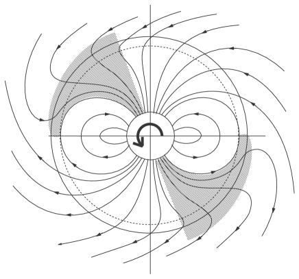
Figure 3: The view from the top of the schematic magnetic field structure of the outflow from an orthogonal rotator with an initially dipole magnetic field. The light cylinder is shown by the solid circle. Direction of rotation is shown by the thick arrow. The region of the closed field lines does not reach the light cylinder and is limited by the dashed circle. Some of the open field lines (shadowed) are curved in the direction of rotation up to the light cylinder. The magnetocentrifugal acceleration will take place on these field lines. Beyond the light cylinder, all the open field lines are curved in the Archimedian spiral typical of axisymmetric outflows.

The schematic structure of an orthogonal rotator with an initially dipole magnetic field is presented in Fig. 3. The dipole magnetic field is not axisymmetric at oblique rotations. There are regions of closed field lines in the magnetosphere and regions of open field lines along which the plasma outflows. Some of these field lines are initially curved in the direction of rotation. Therefore, the new type of MC plasma acceleration discussed in this paper must work under radio pulsar conditions. The question remains, however, whether this mechanism of plasma acceleration essentially changes the energy of the plasma in pulsar conditions.

Real pulsar parameters corresponds to the conditions $R_{a}>R_{L}$ and $R_{a}<\gamma_{0}R_{L}$. So, our solution cannot be directly applied to radio pulsars since it is valid at $R_{a}<R_{L}$. However, this solution can give important qualitative information about the process of wind acceleration in any magnetosphere having violated the condition of axial symmetry.

To understand at least qualitatively the influence of the violation of the axial symmetry on the process of the MC acceleration in a pulsar magnetosphere we should estimate the dimensionless values of the expansion parameters in Eq. (62) for pulsar conditions. If these parameters are small, it would imply that this effect is not important for radio pulsars. If these parameters are of the order of 1, it would imply that the MC acceleration in the pulsar conditions can essentially change the energy of the plasma.

The expansion in Eq. (62) occurs in two parameters $\varepsilon$ and ${\Omega R_{*}\over c}$. $\varepsilon$ can be estimated as $\varepsilon\approx\delta H_{*}/<H_{*}>$ where $\delta H_{*}$ is the maximal variation of the magnetic field on the surface of the star and $<H_{*}>$ is the average magnetic field on the surface of the star. It is evident that $\varepsilon\sim 1$ for dipolar magnetic fields which are believed to occur on the pulsar surface.

In the second dimensionless parameter ${\Omega R_{*}\over c}$, the physical sense of $R_{*}$ is the most unclear. At first glance, it seems that this parameter defines the scale over which the magnetic field decreases with distance from the star. However, more close inspection of Eq. (62) shows that this cannot be correct. The first correction to the Lorentz factor (62) does not depend on the magnetic field $H_{*}$ at all, provided that $3R_{a}^{2}\ll R_{*}^{2}$. Therefore, $R_{*}$ cannot be interpreted as describing the scale of decrease of the magnetic field.

To understand the physical sense of $R_{*}$ in Eq. (62), it is necessary to note that the MC acceleration under consideration occurs only in regions where the magnetic field lines were initially curved into the direction of rotation. Simple analysis of the correction to the magnetic field (47) shows that the violation of axial symmetry on the surface of the star results in the bending of field lines in the region with a characteristic size $R_{*}$. The shape of the field lines does not depends on $H_{*}$ at $3R_{a}^{2}\ll R_{*}^{2}$. This inequality means that the energy density of the magnetic field exceeds the energy density of the plasma near the star surface. At larger distances, the field lines straighten and do not accelerate the plasma. Thus, $R_{*}$ plays the role of the characteristic scale $R_{curve}$ on which the magnetic field lines have nonzero curvature. Only accidentally does $R_{curve}=R_{*}$ in our specific case. Thus, the second parameter defining the expansion of the terminating Lorentz factor can be presented as $\Omega R_{curve}/c$.

In the pulsar magnetosphere, the scale of the poloidal magnetic field variation is equal to the radius of the star, $R_{*}$. The scale $R_{curve}$ depends on the topology of the poloidal magnetic field. In the conventional models, the region of the closed field lines almost reaches the light cylinder. Direct calculations in the axisymmetric model confirm this assumption (Contoupolos et al. [1999]). For this magnetic field topology $R_{curve}\sim R_{L}$ and therefore, the parameter $\Omega R_{curve}/c$ also should be close to 1. For this reason, we conclude that the influence of the violation of the magnetic field axial symmetry on the process of the MC acceleration is certainly not small in the pulsar conditions and it could provide efficient acceleration of the relativistic winds.

It is difficult to estimate reliably the terminating Lorentz factor of the plasma accelerated due to this mechanism in the magnetosphere of pulsars. Any field line initially curved into the direction of rotation is transformed into an Archimedian spiral well beyond the light cylinder where acceleration does not occur. The maximal Lorentz factor is defined by the distance where this transition occurs. This is defined by the field structure at the vicinity of the light cylinder near the last closed field line of the magnetosphere, as is shown in Fig. 3 (shadowed region). Only accurate mathematical solutions will give an accurate answer to questions regarding the terminating Lorentz factor of the plasma. However, it is easy to understand that if this mechanism really provides transformation of the Poynting flux into kinetic energy of the plasma, then the acceleration must take place very close to the light cylinder.

In conclusion, we note that the acceleration of the relativistic winds at the light cylinder of radio pulsars looks attractive from an astrophysical point of view as well. The mechanism of MC acceleration of the plasma which we have described can allow us to resolve a long-standing problem of additional acceleration of the wind from the Crab pulsar. It follows from the comparison of the observations of the Crab Nebula with the MHD theory of the interaction of the pulsar wind with the interstellar medium that the ratio of the Poynting flux to the density of the kinetic energy flux in the wind before the terminating shock is of the order $\sim 10^{-3}$ (Rees & Gunn [1974], Kennel & Coroniti [1984]). However, this ratio cannot be achieved at the dissipativeless axisymmetric outflow(see in particular Chiueh et al.’s (1998) discussion of this question). It was argued recently by Begelman (1998) that the ratio of the Poynting flux to the kinetic energy flux of the order of 1 can also be consistent with the observations of the Crab Nebula if we take into account a possible instability of the flow after the terminating shock. In any case, an additional acceleration of the wind of the relativistic plasma is needed to explain the observations of the Crab Nebula, since the electrostatic gap models are not able to reproduce a wind with the necessary characteristics (Arons [1996]). If we assume that the wind is accelerated due to the MC mechanism and that it carries off approximately half of the total rotational energy of the pulsar in the form of the kinetic energy, this resolves the problem of wind acceleration. The ratio of the Poynting flux to the kinetic energy flux of the plasma appears to be of the order of 1 immediately after the light cylinder, which is consistent with the observations of the Crab Nebula according to Begelman’s scenario (1998). This also resolves the difficulties with the mechanism of the wind acceleration at large distances from the pulsar proposed by Coroniti (1990) and recently revisited by Lyubarskii & Kirk ([2000]). There is simply no need to invoke additional mechanisms in this acceleration.

Analysis performed by Aharonian & Bogovalov (1999) (see also Bogovalov & Aharonian (2000)) shows that the wind from the Crab pulsar with energetics comparable to the total rotational losses of this pulsar and accelerated near the light cylinder should have a total particle flux of $\sim 10^{40}$part./s and an average Lorentz factor of $\sim 10^{5}$ to be consistent with the limitations imposed by observations of the Crab Nebula in VHE gamma-rays. It is interesting that the wind with these parameters indeed provides the total injection rate into the Crab Nebula necessary to explain the electromagnetic emission in the wide range from radio to X-rays (Rees & Gunn [1974]). Thus, the idea that the mechanism of magnetocentrifugal acceleration of the plasma in the axially non uniform magnetic field can be responsible for the acceleration of the wind in the magnetosphere of radio pulsars does not contradict observations of the Crab pulsar and Nebula and deserves further development in a more realistic model.