Cosmic Microwave Background in Closed Multiply Connected Universes

Abstract

We have investigated the cosmic microwave background (CMB) anisotropy in closed multiply connected universes (flat and hyperbolic) with low matter density. We show that the COBE constraints on these low matter density models with non-trivial topology are less stringent since a large amount of CMB anisotropy on large angular scales can be produced due to the decay of the gravitational potential at late time.

Yukawa Institute for Theoretical Physics, Kyoto University,
Kyoto 606–8502, Japan

1 Introduction

For a long time, cosmologists have assumed the simply connectivity of the spatial hypersurface of the universe. If it is the case, the topology of closed 3-spaces is limited to that of a 3-sphere if Poincaré’s conjecture is correct. However, there is no particular reason for assuming the simply connectivity since the Einstein equations do not specify the boundary conditions. If we allow the spatial hypersurface being multiply connected then the spatial geometry of closed models can be flat or hyperbolic as well. We should be able to observe the imprint of the “finiteness” of the spatial geometry if it is multiply connected on scales of the order of the particle horizon or less, in other words, if we live in a “small universe”.
However, it has been claimed by several authors that the “small universes” have already been ruled out observationally. For a flat 3-torus model without the cosmological constant, the COBE data constrains the topological identification scale $L$ (the minimum length of periodic geodesics) to be $L\geq 0.4\times 2R_{\ast}$ where $R_{\ast}$ is the comoving radius of the last scattering surface [1, 2, 3, 4]. The suppression of the fluctuations on scales beyond $L$ leads to a decrease of the angular power spectrum $C_{l}$ of the CMB temperature fluctuations on large angular scales.
In contrast, for low matter density models, the constraint could be considerably less stringent since a bulk of large-angle CMB fluctuations can be produced by the so-called (late) integrated Sachs-Wolfe effect [5] which is the gravitational blueshift effect of the free streaming photons caused by the decay of the gravitational potential[6]. If the background geometry is either flat or hyperbolic, then the angular size of a fluctuation becomes small as it approaches to the observation point. Although fluctuations beyond the size of the fundamental domain are suppressed, no significant suppression in large-angle power occurs if they are produced at place well after the last scattering. In other words, large-angle fluctuations can be generated when the fluctuations enter the topological identification scale at late time.

2 Closed Flat Models

Let us first consider closed models in which the spatial geometry is represented as a flat 3-torus obtained by gluing the opposite faces of a cube with sides $L$ by three translations. Then the wave numbers of the square-integrable eigenmodes of the Laplacian are restricted to the discrete values $k_{i}=2\pi n_{i}/L$, ($i=1,2,3$) where $n_{i}$’s run over all integers. Assuming adiabatic initial perturbation, the angular power spectrum is written as

$$C_{l} = \sum_{{\mathbf{k}}\neq 0}\frac{8\pi^{3}{\cal{P}}_{\Phi}(k)F_{kl}^{2}}{k^{3}L^{3}},$$

$$F_{kl} = \frac{1}{3}\Phi(\eta_{\ast})j_{l}(k(\eta_{o}\!-\!\eta_{\ast}))\!+2\int_{\eta_{\ast}}^{\eta_{o}}\!\!\!\!\!\!d\eta\,\frac{d\Phi}{d\eta}j_{l}(k(\eta_{o}\!-\!\eta)),$$ (1)

where $\eta_{\ast}$ and $\eta_{0}$ correspond to the last scattering and the present conformal time, ${\cal{P}}_{\Phi}(k)$ is the initial power spectrum for the Newtonian curvature perturbation $\Phi$ and $k\equiv\sqrt{k_{1}^{2}+k_{2}^{2}+k_{3}^{2}}$. From now on we assume the scale-invariant Harrison-Zel’dovich spectrum (${\cal{P}}_{\Phi}(k)\!=\!const.$) as the initial power spectrum. The angular scale which gives the suppression scale $l_{cut}$ is determined by the lowest eigenmode on the last scattering surface. The oscillation scale for $l\!<\!l_{cut}$ is also determined by the first eigenmode corresponding to the contribution from ordinary Sachs-Wolfe effect and the integrated Sachs-Wolfe effect. On smaller angular scales $l>l_{cut}$, each peak in the power corresponds to the fluctuation scale of the second and higher eigenmodes at the last scattering. This behavior is analogous to the acoustic oscillation where the oscillation scale is determined by the sound horizon at the last scattering.

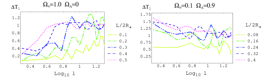
Figure 1: Suppression in large-angle power for 3-torus models with or without the cosmological constant. The significant large-angle suppression in $\Delta T_{l}\equiv\sqrt{l(l+1)C_{l}/(2\pi)}$ (all the plotted values are normalized by $\Delta T_{20}$ with infinite volume) occurs for the “standard” 3-torus model $(\Omega_{m},\Omega_{\Lambda})\!=\!(1.0,0)$ at $l\!<\!l_{cut}\!\sim\!2\pi R_{\ast}/L-1$ while such prominent suppression is not observed for the 3-torus model with ($\Omega_{m},\Omega_{\Lambda}$)=(0.1,0.9).

As shown in figure 1, the angular power for a model with $(\Omega_{m},\Omega_{\Lambda})\!=\!(0.1,0.9)$ is jagged in $l$ but strong suppression is not observed for even very small models. Surprisingly, in low matter density models, the slight excess power due to the integrated Sachs-Wolfe effect is cancelled out by the moderate suppression owing to the mode-cutoff which leads to a nearly flat spectrum. However, as observed in the “standard” 3-torus model, the power spectra have prominent oscillating features.
We have carried out Bayesian analyses using the COBE-DMR 4-year data and obtained the constraints in the size of the fundamental domain $L\geq 1.6H_{0}^{-1}$ and $L\geq 2.2H_{0}^{-1}$ for the “standard” 3-torus model $(\Omega_{m},\Omega_{\Lambda})=(1.0,0)$ and the 3-torus model with low matter density $(\Omega_{m},\Omega_{\Lambda})=(0.1,0.9)$, respectively. The maximum number $N$ of images of the cell within the observable region at present is 8 and 49 for the former and the latter, respectively[7].

3 Closed Hyperbolic Models

Next we consider closed hyperbolic models with small volume. The interesting property of closed (compact) hyperbolic manifolds is the existence of the lower bound for the volume $V\!>\!0.16668...$ (in unit of cube of curvature radius). If the creation of the universe with smaller volume is more likely then it gives the reason why the topological identification scale is comparable to the present horizon scale. For flat models, there is no reason for the “coincidence” in the scale since one can choose the volume arbitrarily. The smallest known one is called the Weeks manifold with volume 0.94 (in unit of cube of curvature radius). Today, the number of known examples of closed hyperbolic manifolds is more than 10000 which have been stored in a computer program “SnapPea” by J. Weeks[8].

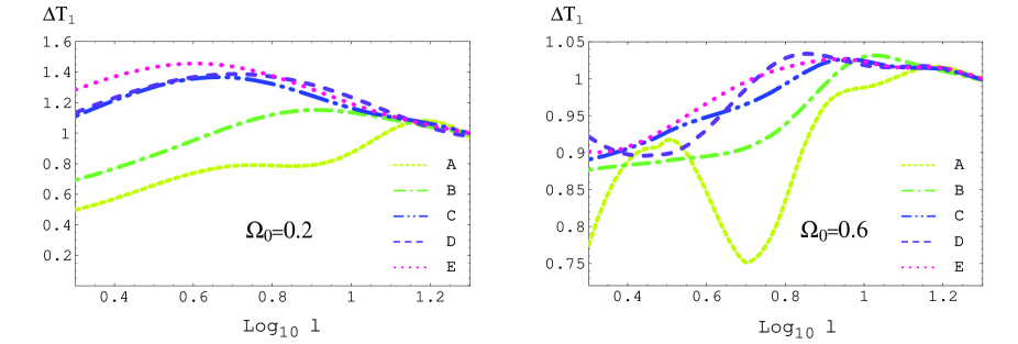
Figure 2: Suppression in large-angle power $\Delta T_{l}\equiv\sqrt{l(l+1)C_{l}/(2\pi)}$ for five closed hyperbolic models (name,volume)=A:(m003(3,-1),0.94), B:(m010(-1,3),1.9), C:(m082(-2,3),2.9), D:(m288(-5,1),3.9) and E:(s873(-4,1), 4.9).

In fact, we have found that the suppression in the angular power due to the mode-cutoff for closed hyperbolic models is also very weak (figure 2). As is the case for flat 3-torus models, the suppression scale $l_{cut}$ is determined by the lowest eigenmode on the last scattering surface. Beyond the scale $l_{cut}$ the ordinary Sachs-Wolfe contribution is strongly suppressed as in compact flat models without the $\Lambda$ term. The weak suppressions imply the significant contribution from the integrated Sachs-Wolfe effect on large-angle scales $l>l_{cut}$. Because the curvature dominant epoch comes earlier in time than the $\Lambda$ dominant epoch, the contribution from the integrated Sachs-Wolfe effect is much greater than that for flat $\Lambda$ models. Below the scale $l_{cut}$, a considerable amount of contribution comes from the second lowest eigenmode. As the number of modes which contribute to $C_{l}$ grows, $C_{l}$ converges to the value for the infinite counterpart. The obtained constraint for the Weeks model (volume=0.94) is $\Omega_{0}\geq 0.1$ and the maximum expected number of copies of the fundamental domain inside the present observable region is approximately 1560. Note that the obtained result agrees with other recent works[12, 13, 14]. Furthermore, for some closed hyperbolic models, it is found that the computed angular powers give a much better fit to the COBE data since the quadrapole is very low.
However, one might argue that the constraint using only the power spectrum is not sufficient since it contains only isotropic information for 2-point correlations[9]. In fact there is a gap between the likelihood using only the power spectrum and that using full covariance elements for the 3-torus models[7]. For globally anisotropic models, the fluctuations are anisotropic Gaussian for a given axis but are non-Gaussian if the likelihoods are marginalized over the axis. For locally closed Friedmann-Robertson-Walker models, the skewness is zero but the kurtosis is non-zero assuming that the initial fluctuations are Gaussian. Another feature is the correlation between the expansion coefficient $a_{lm}$’s of the temperature fluctuations in the sky which are independent random numbers for the standard infinite counterparts in which the initial fluctuations are homogeneous and isotropic Gaussian. In the case of flat 3-torus models, $a_{lm}$’s are written in terms of spherical harmonics $Y_{lm}(\hat{\mathbf{k}})$ which correspond to the expansion coefficients of the eigenmodes in the 3-torus in terms of the eigenmodes of the 3-dimensional Euclidean space. Therefore, if the number of the term in the sum that gives $a_{lm}$ is small then $a_{lm}$’s are no longer independent. This is the main reason for the gap in the likelihoods for the 3-torus models. In contrast, for closed hyperbolic models, the expansion coefficients of the eigenmodes are well approximated by Gaussian pseudo random numbers [10, 11]. Therefore for homogeneous ensembles, $a_{lm}$ can be described as independent “random” numbers although they are non Gaussian (since they are written in terms of a sum of products of two independent Gaussian numbers). This implies that the value of the likelihood is highly dependent on the place of the observer in the manifold. In order to constrain closed hyperbolic models which are globally inhomogeneous, one should calculate the likelihood everywhere in the manifold. If one marginalizes the likelihood over the orientation (axis) and the position of the observer then $a_{lm}$’s become independent non-Gaussian random numbers. Thus we expect that the constraints using only the power spectrum give better estimates for closed hyperbolic models than closed flat models in which the correlations in $a_{lm}$’s are prominent.

4 Conclusion

We have investigated the CMB anisotropy in closed multiply connected universes (flat and hyperbolic) with low matter density. We have seen that the COBE constraints for these models are less stringent compared with the simplest “standard” 3-torus model ($\Omega_{m}\!=\!1.0$). On the other hand recent observations of distant supernova Ia [15, 16] and of the CMB on small angular scales [17, 18] imply that our universe is nearly flat with the cosmological constant (or “quintessence”, X-matter etc.) which dominates the present universe. It seems that the closed hyperbolic models are ruled out but it is still not conclusive. If one includes the cosmological constant for a fixed curvature radius, the comoving radius of the last scattering surface in unit of curvature radius becomes large. Therefore the observable effects of the non-trivial topology become much prominent. For instance, the number $N$ of copies of the fundamental domains inside the observable region at present is approximately 28 for the Weeks model with $\Omega_{\Lambda}\!=\!0.6$ and $\Omega_{m}\!=0.2\!$ whereas $N\!=\!4$ if $\Omega_{\Lambda}\!=\!0$ and $\Omega_{m}\!=0.8\!$. If one allows hyperbolic orbifold models then the number can be increased as much as $N=52$ for $\Omega_{\Lambda}\!=\!0.75$ and $\Omega_{m}\!=\!0.2$ since the volume of the smallest orbifold (arithmetic) is very small (=0.039). At least at the classical level it seems that there is no reason to exclude any orbifold models although they have singular points where the curvature diverges.

References

- [1] I.Y. Sokolov, JETP Lett. 57 (1993) 617.
- [2] A.A. Starobinsky, JETP Lett. 57 (1993) 622.
- [3] D. Stevens, D. Scott and J. Silk, Phys. Rev. Lett. 71 (1993) 20.
- [4] A. de Oliveira-Costa, G.F. Smoot, Astrophys. J. 448 (1995) 447.
- [5] N. Cornish and D. Spergel, Phys. Rev. D 57 (1998) 5982.
- [6] W. Hu, N. Sugiyama and J. Silk, Nature 386 (1997) 37.
- [7] K.T. Inoue, astro-ph/0011462.
- [8] J.R. Weeks, SnapPea, A Computer Program for Creating and Studying Hyperbolic 3-manifolds, available at: http://www.northnet.org/weeks
- [9] J.R. Bond, D. Pogosyan and T. Souradeep, Phys. Rev. D 62 (2000) 043006.
- [10] K.T. Inoue, Class. Quantum Grav. 16 (1999) 3071.
- [11] K.T. Inoue, Phys. Rev. D 62, (2000) 103001.
- [12] R. Aurich, Astrophys. J. 524 (1999) 497.
- [13] N.J. Cornish and D.N. Spergel, Phys. Rev. D 62 (2000) 087304.
- [14] R. Aurich and F. Steiner, astro-ph/0007264.
- [15] S. Perlmutter et al, Astrophys. J. 517 (1999) 565.
- [16] A. Riess et al, Astron. J. 117 (1999) 707.
- [17] A. Melchiorri et al, Astrophys. J. 536 Issue 2 (2000) L63.
- [18] A. Balbi et al, astro-ph/0005124 acceped in Astrophys. J. Letters (2000).