Compton Scattering in Static and Moving Media.
II. System-Frame Solutions for Spherically Symmetric Flows

Abstract

I study the formation of Comptonization spectra in spherically symmetric, fast moving media in a flat spacetime. I analyze the mathematical character of the moments of the transfer equation in the system-frame and describe a numerical method that provides fast solutions of the time-independent radiative transfer problem that are accurate in both the diffusion and free-streaming regimes. I show that even if the flows are mildly relativistic ($V\sim 0.1$, where $V$ is the electron bulk velocity in units of the speed of light), terms that are second-order in $V$ alter the emerging spectrum both quantitatively and qualitatively. In particular, terms that are second-order in $V$ produce power-law spectral tails, which are the dominant feature at high energies, and therefore cannot be neglected. I further show that photons from a static source are upscattered by the bulk motion of the medium even if the velocity field does not converge. Finally, I discuss these results in the context of radial accretion onto and outflows from compact objects.

1 INTRODUCTION

Compton scattering in quasi-spherical accretion flows is thought to be responsible for the X-ray spectra of many accreting compact objects. For example, the hard X-ray spectra of weakly-magnetic accreting neutron stars can be accounted for if a geometrically thick, hot medium surrounds the neutron star and inner accretion disk (see, e.g., Psaltis, Lamb, & Miller 1995). The spectral signature of isolated neutron stars accreting from the interstellar medium, which is required for their positive identification, is determined mainly by the efficiency of Compton upscattering of thermal photons emitted from the stellar surfaces (see, e.g., Zampieri et al. 1995). Moreover, Compton scattering plays a major role in the formation of the high-energy spectra of advection-dominated accretion flows, which may be the relevant mode of accretion onto galactic and supermassive black holes (see, e.g., Esin et al. 1997).

Compton scattering in static and moving media, even in plane-parallel or spherical symmetry, couples strongly all three independent phase-space coordinates of the photons, namely their energy, direction of propagation, and spatial coordinate. For this reason, Monte Carlo methods have been used extensively in calculating Comptonization spectra, because of their easy implementation and natural treatment of the diverse length scales in an accretion flow (see, e.g., Laurent & Titarchuk 1999 for a recent study; methods and results based on Monte Carlo treatments have been reviewed by Pozdnyakov, Sobol, & Sunyaev 1983 and will not be discussed here). Alternatively, Compton scattering can be studied by solving the energy-dependent radiative transfer equation or its moments. Implementing such a method is more difficult and often relies on a number of approximations for describing the interaction of radiation with matter (see, however, Poutanen & Svensson 1996 and Hsu & Blaes 1998 for complete solutions in static media). However, at the same time it is substantially faster and offers significant advantages when the radiative transfer problem is coupled to a solution of the fluid dynamics, as well as in treating steep spectra and processes that do not conserve photons.

Over the last twenty five years several authors have derived the photon kinetic or radiative transfer equation and their moments for Compton scattering in static and moving media (see, e.g., Kompaneets 1957; Babuel-Peyrissac & Rouvillois 1969; Pomraning 1973; Chan & Jones 1975; Payne 1980; Blandford & Payne 1981a; Thorne 1981; Fukue, Kato, & Matsumoto 1985; Madej 1989, 1991; Titarchuk 1994). The moment equations derived by these various sets of authors have been widely used in studies of Comptonization by static media (see, e.g., Katz 1976; Shapiro, Lightman, & Eardly 1976; Sunyaev & Titarchuk 1980) or by strong shocks and accretion flows onto compact objects (see, e.g., Blandford & Payne 1981b; Payne & Blandford 1981; Lyubarskij & Sunyaev 1982; Colpi 1988; Riffert 1988; Mastichiadis & Kylafis 1992; Titarchuk & Lyubarskij 1995; Turolla et al. 1996; Titarchuk, Mastichiadis, & Kylafis 1997), either under the diffusion approximation or with closure relations that were specified a priori. Most of the above analyses of Compton scattering in moving media were performed in the system frame and to first order in the electron bulk velocity. On the other hand, Schmid-Burgk (1978), Zane et al. (1996), and Titarchuk & Zannias (1998) have solved the general-relativistic radiative transfer equation for Compton scattering without the need for specifying a priori closure relations.

In Paper I (Psaltis & Lamb 1997) of this series, the time-dependent photon kinetic and radiative transfer equations were derived, as well as their zeroth and first moments that describe absorption, emission, and spontaneous and induced Compton scattering in static and moving media, correcting various errors in the literature. The system-frame equations that were derived are valid to first order in $\epsilon/m_{e}$ and $T_{e}/m_{e}$, and to second order in $V$, where $m_{e}$ and $T_{e}$ are the electron mass and temperature, $\epsilon$ is the photon energy, and $V$ is the bulk velocity of the electrons in units of the speed of light; the fluid-frame equations that were derived are valid for arbitrary values of the bulk velocity $V$. Using these equations it was argued in Paper I that the effects of Comptonization by the bulk electron velocity that are described by the terms that are second-order in $V$ are qualitatively different than and can become at least as important as the effects described by the terms that are first-order in $V$, even when $V$ is small. As a result, these second-order terms should generally be retained (see also Yin & Miller 1995).

In this paper, I describe a numerical algorithm for the solution of time-independent radiative transfer problems in systems with spherical symmetry. Even though the natural reference frame for solving transport problems is the one comoving with the flow, I work in the system frame, which can be any inertial frame in which the central object is at rest. This is important for the fast algorithm described below, because the moment equations in the system frame are always parabolic (as shown in §3) in contrast to the fluid-frame equations (Turolla, Zampieri, & Nobili 1995; Smit, Cernohorsky, & Dullemond 1997; see also Körner & Janka 1992). Moreover, in problems of mass accretion onto a compact star, the boundary conditions are often more easily implemented in the system frame. I also neglect any general relativistic effects, which can be shown to introduce only small quantitative corrections to the emerging spectra (Papathanassiou & Psaltis 2000), and truncate the transfer equation keeping only terms up to second order in $V$.

The algorithm used is a generalization of the method of variable Eddington factors (Mihalas 1980; see also Mihalas 1978, p. 157–158). It is therefore accurate for systems of arbitrary optical depth and does not require a priori specification of closure relations. It is based on the iterative solution of both the transfer equation and the systems of its first two moments and hence the validity and accuracy of the solution can be verified explicitly at the end of each run. The method also requires only a small number of iterations in order to converge to the solution and is therefore ideal for future extensions to time-dependent and multi-dimensional transport problems.

In §2, I summarize the results from Paper I and introduce the notation. In §3, I discuss the mathematical character of the system of equations and in §4, I present the numerical algorithm. In §5, I describe the results of numerical solutions of the transfer equations for a variety of situation. Finally, in §6, I briefly summarize the implications of the above for Comptonization spectra in static and moving media.

2 THE ELECTRON GAS AND RADIATION FIELD

Units—Throughout this paper I set $h=k_{\rm B}=c=1$, where $h$ is Planck’s constant, $k_{\rm B}$ is Boltzmann’s constant, and $c$ is the speed of light. I also normalize all the spatial coordinates to the inner radius of the flow, the electron temperature $T_{e}$ and photon energy $\epsilon$ to the electron rest mass $m_{e}$, and the electron density $n_{e}$ to its value at the inner radius of the flow. Finally, I normalize the emission and absorption coefficients $\eta(r,\epsilon)$ and $\chi(r,\epsilon)$ to the inverse of the electron scattering mean-free path in the Thomson limit.

The electron gas—Let $\vec{u}$ be the system-frame three-velocity of a given electron. I define the local bulk velocity $\vec{V}$ of the electrons measured in the system frame as

$$\vec{V}\equiv\langle\vec{u}\rangle\;,$$ (1)

where the sharp brackets indicate the average over the local electron velocity distribution. I also assume that the electron velocity distribution in the fluid frame is a relativistic Maxwellian and therefore

$$\langle u^{2}\rangle\simeq V^{2}+3T_{e}\;,$$ (2)

where I have neglected terms of order $V^{2}T_{e}$ and higher.

The radiation field—I describe the radiation field at any position in the system frame with coordinate vector $\vec{r}$ using the monochromatic specific intensity $I(\vec{r},\hat{l},\epsilon)$, where $\hat{l}$ is the direction of propagation and $\epsilon$ is the photon energy. Here I consider only unpolarized radiation and hence I have suppressed the dependence of the specific intensity on polarization. Because of the assumed spherical symmetry of the problem, the radiation field depends only on the radial distance from the center of symmetry (i.e., the $r$–component of the vector $\vec{r}$), on the angle $\theta$ between the radial direction and the direction of propagation (i.e., $\cos\theta=\hat{l}\cdot\vec{r}/r$), and on the photon energy $\epsilon$.

I define the first five moments of the monochromatic specific intensity as

$$J(\vec{r},\epsilon) \equiv \frac{1}{4\pi}\int_{\Omega}I(\vec{r},\hat{l},\epsilon)d\Omega$$ (3)

$$H^{i}(\vec{r},\epsilon) \equiv \frac{1}{4\pi}\int_{\Omega}I(\vec{r},\hat{l},\epsilon)l^{i}d\Omega$$ (4)

$$K^{ij}(\vec{r},\epsilon) \equiv \frac{1}{4\pi}\int_{\Omega}I(\vec{r},\hat{l},\epsilon)l^{i}l^{j}d\Omega$$ (5)

$$Q^{ijk}(\vec{r},\epsilon) \equiv \frac{1}{4\pi}\int_{\Omega}I(\vec{r},\hat{l},\epsilon)l^{i}l^{j}l^{k}d\Omega$$ (6)

$$R^{ijkl}(\vec{r},\epsilon) \equiv \frac{1}{4\pi}\int_{\Omega}I(\vec{r},\hat{l},\epsilon)l^{i}l^{j}l^{k}l^{l}d\Omega\;.$$ (7)

The non-zero components of the first five moments of the specific intensity for systems with spherical symmetry are given in Appendix A.

The transfer equation and its moments—Following Mihalas (1980; see also Mihalas 1978), I solve the radiative transfer equation in a plane that contains the center of symmetry of the system, between the inner and outer radii $r_{\rm in}$ and $r_{\rm out}$ of the flow, using the coordinates $z\equiv r\cos\theta$ and $p\equiv r\sin\theta$.

The radiative transfer equation along a ray of constant impact parameter $p$ is

$$\pm\frac{\partial}{\partial\tau_{z}}I^{\pm}(z,p,\epsilon)=(1-2\epsilon)I^{\pm}(z,p,\epsilon)-S^{\pm}(z,p,\epsilon)\;,$$ (8)

where the signs ‘$+$’ and ’$-$’ correspond to the equations for the outgoing and incoming rays respectively and I have neglected the effects of induced Compton scattering. In equation (8) I have used the optical depth along the ray defined as $d\tau_{z}\equiv-n_{e}\sigma_{T}[1+\chi(r,z,\epsilon)]dz$, where $\tau_{z}=0$ at the outer boundary and $\sigma_{T}$ is the angle-integrated Thomson scattering cross section. $S^{\pm}(z,p,\epsilon)$ is the generalized source function for absorption, emission, and Compton scattering in systems with spherical symmetry and is given in Appendix B.

The equations for the moments of the specific intensity can be derived either directly from equation (8) or from equations (34) and (40) of Paper I. Written in compact form and using the dimensionless quantities defined above, the moment equations are

$$A_{1}J+A_{2}\epsilon\partial_{\epsilon}J+A_{3}\epsilon^{2}\partial^{2}_{\epsilon}J+A_{4}H^{r}+A_{5}\epsilon\partial_{\epsilon}H^{r}+\partial_{\tau_{r}}H^{r} = C_{1}$$ (9)

$$B_{1}J+B_{2}\epsilon\partial_{\epsilon}J+f^{rr}\partial_{\tau_{r}}J+B_{3}H^{r}+B_{4}\epsilon\partial_{\epsilon}H^{r}+B_{5}\epsilon^{2}\partial^{2}_{\epsilon}H^{r} = C_{2}\;,$$ (10)

where $\partial_{\epsilon}\equiv\partial/\partial\epsilon$, $\partial^{2}_{\epsilon}\equiv\partial^{2}/\partial\epsilon^{2}$, $\partial_{\tau_{r}}\equiv\partial/\partial\tau_{r}$, and $\tau_{r}\equiv-\sigma_{T}n_{e}(r_{\rm in})(r-r_{\rm out})$. When the electron density is uniform, then the dimensionless quantity $\tau_{r}$ is equal to the electron scattering optical depth in the radial direction measured from $r_{\rm out}$. The coefficients in equations (9) and (10) are given in Appendix C.

Boundary Conditions—The boundary conditions for both the transfer equation and the system of its moments depend on the specific problem under study. For the model problems discussed in §5, I shall assume that the flow is not illuminated from the outside, i.e.,

$$I^{-}(r_{\rm out},\theta,\epsilon)=0$$ (11)

at the outer boundary, and specify the radiation flux at the inner boundary as

$$I^{+}(r_{\rm in},\theta,\epsilon)=I^{-}(r_{\rm in},\theta,\epsilon)+4H^{r}_{0}(\epsilon)\;.$$ (12)

For solving the moments of the radiative transfer equation I shall specify, for all photon energies $\epsilon$, the first moment of the monochromatic specific intensity at the inner radius, i.e.,

$$H^{r}(r_{\rm in},\epsilon)=H^{r}_{0}(\epsilon)$$ (13)

as well as the ratio of the first to the zeroth moment of the monochromatic specific intensity at the outer radius

$$\frac{H^{r}(r_{\rm out},\epsilon)}{J(r_{\rm out},\epsilon)}=k(\epsilon)\;.$$ (14)

The quantity $k(\epsilon)$ is not known a priori but is calculated in a self-consistent way in the iterative method described below. I shall also set at all radii

$$\lim_{\epsilon\rightarrow 0}J(r,\epsilon)=\lim_{\epsilon\rightarrow\infty}J(r,\epsilon)=0$$ (15)

and

$$\lim_{\epsilon\rightarrow 0}H^{r}(r,\epsilon)=\lim_{\epsilon\rightarrow\infty}H^{r}(r,\epsilon)=0\;,$$ (16)

which reflect the fact that the photon occupation number and the radiation flux are finite quantities.

3 MATHEMATICAL CHARACTER OF THE MOMENT EQUATIONS

In the method of variable Eddington factors, the system of partial differential equations (9) and (10) is solved iteratively with the radiative transfer equation (8), given a set of Eddington factors computed from the previous iteration. The boundary conditions and the method used for the solution of the system depends on the character of the partial differential operator. For example, the system of moment equations in the frame comoving with the flow (or the local Lorentz frame when gravitational effects are taken into account) may be hyperbolic or elliptic, depending on the velocity field (Turolla et al. 1995). In this section I follow the procedure outlined by Ames (1992, pp. 8–12) to show that the system-frame, energy dependent moment equations always form a parabolic system of partial differential equations, thus simplifying the implementation of the numerical algorithm.

I define the quantities $L=\partial_{\epsilon}J$ and $M^{r}=\partial_{\epsilon}H^{r}$, which together with the partial differential equations (9) and (10), and the equations for the differentials $dJ$, $dH^{r}$, $dL$, and $dM^{r}$, form an $8\times 8$ system of algebraic equations for the eight derivatives

$$\left[\begin{array}[]{cccccccc}1&0&0&0&0&0&0&0\\ 0&0&1&0&0&0&0&0\\ 0&0&0&1&A_{3}\epsilon^{2}&0&0&0\\ 0&f^{rr}&0&0&0&0&B_{5}\epsilon^{2}&0\\ 0&d\tau_{r}&0&0&0&0&0&0\\ 0&0&0&d\tau_{r}&0&0&0&0\\ 0&0&0&0&d\epsilon&d\tau_{r}&0&0\\ 0&0&0&0&0&0&d\epsilon&d\tau_{r}\end{array}\right]\cdot\left[\begin{array}[]{c}\partial_{\epsilon}J\\ \partial_{\tau_{r}}J\\ \partial_{\epsilon}H^{r}\\ \partial_{\tau_{r}}H^{r}\\ \partial_{\epsilon}L\\ \partial_{\tau_{r}}L\\ \partial_{\epsilon}M^{r}\\ \partial_{\tau_{r}}M^{r}\\ \end{array}\right] =$$ (33)

$$\qquad\qquad\qquad\qquad\qquad\qquad=\left[\begin{array}[]{c}L\\ M^{r}\\ C_{1}-A_{1}J-A_{2}\epsilon L-A_{4}H^{r}-A_{5}\epsilon M^{r}\\ C_{2}-B_{1}J-B_{2}\epsilon L-B_{3}H-B_{4}\epsilon M^{r}\\ dJ-Ld\epsilon\\ dH^{r}-M^{r}d\epsilon\\ dL\\ dM^{r}\end{array}\right]\;.$$ (34)

Equating the determinant of the coefficient matrix to zero, I obtain the characteristic equation for the system of equations,

$$A_{3}B_{5}\epsilon^{4}\left(d\tau_{r}\right)^{4}=0\;.$$ (35)

The coefficients $A_{3}$ and $B_{5}$ are proportional to the electron temperature and the square of the bulk velocity (see Appendix C) and hence for the problems under consideration they are never zero. Therefore, for a finite electron energy $\epsilon$, the system of partial differential equations (9) and (10) has only one multiple, real characteristic direction, i.e., $d\tau_{r}=0$, and hence is always parabolic. The difference with respect to the moment equations in the comoving frame arises from the presence of second order energy derivatives in the differential operator.

4 NUMERICAL METHOD

Equation (8) is an integro-differential equation for the specific intensity of the radiation field and therefore any numerical solution of this equation is not trivial to obtain. On the other hand, the system of equations (9) and (10) depends on two variable Eddington factors and an unknown outer boundary condition, which can be computed only when the solution of equation (8) for the specific intensity is obtained. Here, I employ a numerical algorithm that is a generalization of the method of variable Eddington factors (Mihalas 1980; see also Mihalas 1978, pp. 157–158) in order to solve iteratively equation (8) for the specific intensity of the radiation field and the system of partial differential equations (9) and (10) for its zeroth and first moments. This algorithm has been proven to be very efficient and gives a solution to the complete transfer equation that is limited only by numerical accuracy, independent of the optical depth of the medium.

In this method, I first solve the moments of the transfer equation using an initial guess for the variable Eddington factors and for the outer boundary condition. I then compute the generalized source function using the calculated moments of the specific intensity, solve the radiative transfer equation, and use this solution to update the Eddington factors. I repeat the whole procedure until convergence is achieved.

4.1 Solution of the Moments of the Transfer Equation

The moments of the transfer equation depend only on radius and photon energy, when the variable Eddington factors are known. Therefore, I discretize the domain of solution and the differential operators of equations (9) and (10) on a two–dimensional mesh of $N_{\tau}$ grid points over the variable $\tau_{r}$ and $N_{En}$ grid points over the photon energy $\epsilon$.

The mesh of discrete grid points over the variable $\tau_{r}$ must resolve the rapid change of the variable Eddington factors with optical depth near both boundaries of the domain of solution. In order to achieve this, I define the mesh points to be equidistant in the quantity

$$Q=\left\{\begin{array}[]{ll}W\tau+(1-W)\log\tau\;,&\quad\quad\tau\leq\frac{1}{2}\tau_{m}\\ W\left(\tau_{m}-\tau\right)+(1-W)\log\left(\tau_{m}-\tau\right)&\quad\quad\tau\geq\frac{1}{2}\tau_{m}\end{array}\right.\;,$$ (36)

where $\tau$ is the total optical depth (and not the quantity $\tau_{r}$) in the radial direction measured from $r_{\rm out}$, $\tau_{m}\equiv\tau(r_{in})$ is the maximum radial optical depth in the medium, and $W$ is a parameter that allows a combination of a logarithmic grid near the boundaries with a linear grid in the interior. Because the spectra that emerge from Comptonizing media are usually power laws, I use a logarithmic mesh of discrete grid points over photon energy $\epsilon$.

The system of moment equations involve differentiation over two density-like quantities, the radiation energy density $J$ and the first Eddington factor $f^{rr}$, and two flux-like quantities, the radiation energy flux $H^{r}$ and the second Eddington factor $g^{rr}$. I discretize density-like quantities in a shell-centered fashion and flux-like quantities on the grid points. Let $F_{ij}$ be the value of a physical quantity at the $i$–th grid point in the variable $\tau_{r}$ and the $j$–th grid point in photon energy. Away from the boundaries, I differentiate density-like quantities over the variable $\tau_{r}$ on the grid points as

$$\left(\frac{\partial F}{\partial\tau_{r}}\right)_{i,j}=2\frac{F_{i+1/2,j}-F_{i-1/2,j}}{(\tau_{r})_{i+1}-(\tau_{r})_{i-1}}\;,$$ (37)

and flux-like quantities as

$$\left(\frac{\partial F_{ij}}{\partial\tau_{r}}\right)_{i+1/2,j}=\frac{F_{i+1,j}-F_{i,j}}{(\tau_{r})_{i+1}-(\tau_{r})_{i}}\;,$$ (38)

in an explicit or fully implicit scheme.

In both equations I approximate the first derivative of a physical quantity $F$ with respect to photon energy by

$$\left(\frac{\partial F}{\partial\epsilon}\right)_{ij}=\frac{F_{i,j+1}-F_{i,j-1}}{\epsilon_{j+1}-\epsilon_{j-1}}\;.$$ (39)

and the second derivative with respect to photon energy by

$$\left(\frac{\partial^{2}F}{\partial\epsilon^{2}}\right)_{ij}=\frac{2}{\epsilon_{j+1}-\epsilon_{j-1}}\left(\frac{F_{i,j+1}-F_{i,j}}{\epsilon_{j+1}-\epsilon_{j}}-\frac{F_{i,j}-F_{i,j-1}}{\epsilon_{j}-\epsilon_{j-1}}\right)\;,$$ (40)

where the index ‘$i$’ in the quantity $F_{ij}$ may also be fractional, corresponding to a shell center, as needed by an implicit differencing scheme over the variable $\tau_{r}$. The energy differencing scheme (39)–(40) cannot be used directly in differencing the radiation energy density and flux in equations (9) and (10) because it does not guarantee particle conservation when only scattering is taken into account (Chang & Cooper 1970). This is important when the energy spectrum has reached quasi-equlibrium and small numerical errors lead to significant deviation from particle conservation (see eq. [10] in Chang & Cooper 1970). A better differencing scheme can be deduced by examining the properties of the differential operator at that limit.

The solution of the moment equations reaches quasi-equlibrium when the photon mean free path is very small compared to any characteristic length scale in the system. In that limit, $f^{rr}=1/3+{\cal O}(V)$, and when only processes that conserve photon number are operating, the moment equation of zeroth order becomes

$$\left(\partial_{r}+\frac{2}{r}\right)\frac{H^{r}}{\epsilon}=n_{e}\sigma_{\rm T}\partial_{\epsilon}\left[VH^{r}+(\epsilon-3T_{e}-V^{2})J+\left(T_{e}+\frac{V^{2}}{3}\right)\epsilon\partial_{\epsilon}J\right]\;,$$ (41)

where $n_{e}$ is the dimensional electron density. The photon number flux is simply equal to $N^{r}\equiv H^{r}/\epsilon$ and integrating equation (41) over photon energy gives

$$\left(\partial_{r}+\frac{2}{r}\right)\int_{\epsilon}N^{r}d\epsilon=0\;,$$ (42)

i.e., photon conservation. Following Chang & Cooper (1970), I define a generalized photon current ${\cal F}(r,\epsilon)$ as

$${\cal F}(r,\epsilon)=VH^{r}+(\epsilon-3T_{e}-V^{2})J+\left(T_{e}+\frac{V^{2}}{3}\right)\epsilon\partial_{\epsilon}J$$ (43)

and write the zeroth and first moment equations as

$$A_{1}^{\prime}J+A_{2}^{\prime}\epsilon\partial_{\epsilon}J+A_{3}^{\prime}\epsilon^{2}\partial^{2}_{\epsilon}J+A_{4}^{\prime}H^{r}+\partial_{\tau_{r}}H^{r} = C_{1}+n_{e}\epsilon\partial_{\epsilon}{\cal F}$$ (44)

$$B_{1}J+B_{2}\epsilon\partial_{\epsilon}J+f^{rr}\partial_{\tau_{r}}J+B_{3}H^{r}+B_{4}\epsilon\partial_{\epsilon}H^{r}+B_{5}\epsilon^{2}\partial^{2}_{\epsilon}H^{r} = C_{2}\;,$$ (45)

where the coefficient are given in Appendix D. Differencing equations (44)–(45) according to the scheme (37)–(40) results in strict photon number conservation in the limit of small photon mean free paths.

A final point with the energy differencing is related to the requirement that the photon energy density is everywhere positive. This introduces a restriction on the spacing of the energy grid, depending on the differencing scheme. For the scheme used above it can be shown that the requirement for a positive photon energy density results in the restriction (cf. eq. [41] and Chang & Cooper 1970, eq. [14])

$$\frac{\Delta\epsilon}{\epsilon}<\left(\frac{1}{2}\right)\frac{T_{e}+V^{2}/3}{|\epsilon-3(T_{e}+V^{2}/3)|}<\left\{\begin{array}[]{ll}1/6\;,&\qquad\epsilon\ll 3T_{e}+V^{2}\\ \left(\frac{1}{2\epsilon}\right)(T_{e}+V^{2}/3)\;,&\qquad\epsilon\gg 3T_{e}+V^{2}\end{array}\right.\;,$$ (46)

which can be easily met.

I solve the system of equations (44) and (45) for the zeroth and first moments of the specific intensity of the radiation field, $J$ and $H^{r}$, in $N_{\tau}$ grid points in optical depth and $N_{\rm En}$ grid points in photon energy. Therefore the system of equations has $N_{\tau}\times N_{\rm En}$ unknowns. In all the interior grid points ($1<i<N_{\tau}$; $1<j<N_{\rm En}$) I solve both equations (44) and (45) using the differencing scheme of equations (37)–(40). For the inner spatial boundary, i.e., for $i=1$ and for all $j$, I solve equations (13) and (45), whereas for the outer spatial boundary, i.e., for $i=N_{\tau}$ and for all $j$, I solve equations (14) and (44). Finally, at both energy boundaries, i.e., for all $i$ and for $j=1,N_{En}$, I set both the zeroth and first moments of the specific intensity equal to zero, according to boundary conditions (15) and (16).

The resulting system of equations is linear in both the zeroth and first moments of the specific intensity. Defining the quantity $P_{i}$ as

$$\begin{array}[]{ccccc}P_{1}=J_{1,1}\;;&P_{2}=H^{r}_{1,1}\;;&...&P_{2N_{\tau}-1}=J_{N_{\tau},1}&P_{2N_{\tau}}=H^{r}_{N_{\tau},1}\\ \end{array}\quad\mbox{etc.}$$ (47)

the system of equations takes the form shown in Figure 1. The matrix of coefficients is a sparse matrix and can be solved efficiently with the biconjugate gradient method (see, e.g., Press et al. 1992, pg. 209) with a preconditioner matrix. I choose the preconditioner matrix to be the coefficient matrix, with the elements at the outer two diagonal bands set equal to zero. The preconditioner matrix can then be inverted efficiently with the LU-decomposition method (see, e.g., Press et al. 1992, pg. 202). In this method, in order to avoid round-off errors, I scale all the rows in the coefficient matrix so that the highest value of the elements in each row is unity. Depending on the complexity of the particular problem, the system of difference equations can be solved to a fractional accuracy of $10^{-5}$ within less than fifty iterations, which can be performed in a few seconds on a current workstation.

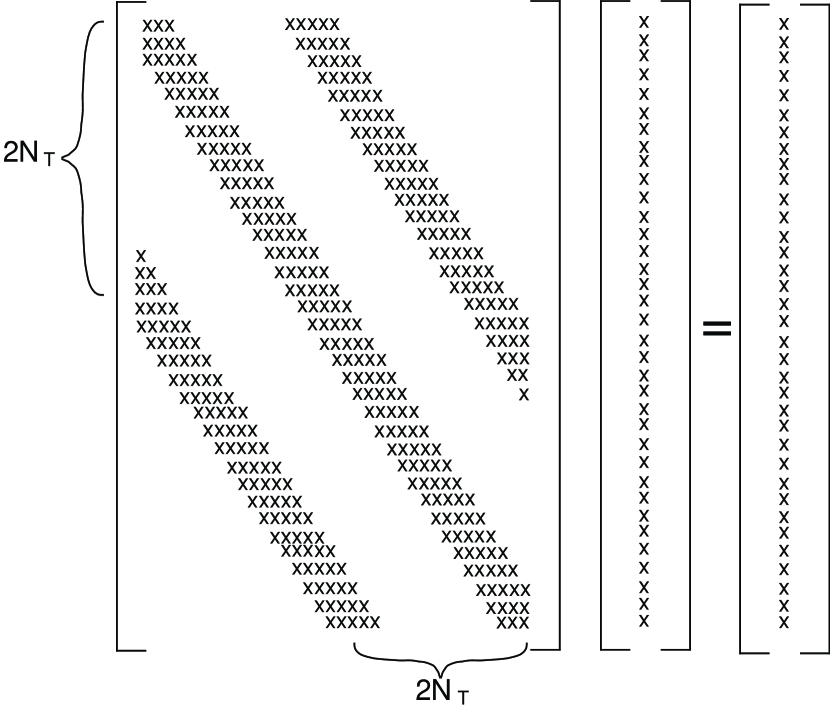
Figure 1: Schematic representation of the linear system of the discretized zeroth and first moments of the radiative transfer equation.

4.2 Solution of the Radiative Transfer Equation

In the iterative method of the variable Eddington factors, the transfer equations (8) is solved at every grid point in the $(p-z)$ plane for the boundary conditions (11) and (12). Because the generalized source function is calculated using the results from the previous iterations, the solution of equation (8) is just the formal solution that can be obtained analytically, i.e.,

$$I^{-}(\tau_{z},p,\epsilon) = \int_{0}^{\tau_{z}}S(t,p,\epsilon)e^{(1-2\epsilon)(t-\tau_{z})}dt$$

$$I^{+}(\tau_{z},p,\epsilon) = I^{+}(z_{\rm min},p,\epsilon)e^{(1-2\epsilon)(\tau_{z}-\tau_{zmin})}$$ (48)

$$\qquad\qquad+\int^{\tau_{zmin}}_{\tau_{z}}S(t,p,\epsilon)e^{(1-2\epsilon)(\tau_{z}-t)}dt\;,$$

where

$$I^{+}(z_{\rm min},p,\epsilon)=\left\{\begin{array}[]{ll}I^{-}(z_{\rm min},p,\epsilon)\;,&p>r_{\rm in}\\ I^{-}(z_{\rm min},p,\epsilon)+4H^{r}_{0}(\epsilon)\;,&p<r_{\rm in}\end{array}\right.$$ (49)

and $z_{min}=0$ or $z_{min}=(r_{\rm in}^{2}-p^{2})^{1/2}$ when $p>r_{\rm in}$ or $p<r_{\rm in}$ respectively. In calculating the integrals in equation (48), I use a piece-wise linear interpolation of the source function through each shell and evaluate the energy derivatives according to equations (39)–(40).

Figure 2: Maximum fractional error in the radiation energy density after each iteration, for the test problems discussed in §4.3.

4.3 Convergence and Validation

The rapid convergence of the method of variable Eddington factors is preserved in the current implementation for the problem of Compton scattering. This is shown in Figure 2, where the maximum fractional error in the radiation energy density is plotted for each iteration, for two uniform media with different scattering optical depths. For the model problems shown, the outer radius of the scattering medium is set to $3r_{\rm in}$, its electron temperature to 10 keV, and the energy-dependence of the radiation flux at the inner boundary to be that of a blackbody with a temperature of 0.5 keV. The converge is typically faster for problems with higher optical depths, because I have used $f^{rr}=1/3$ as an initial value for the first variable Eddington factor, which is closer to the real value at the limit of high optical depth.

The numerical method described in this section also allows for a consistency check between the solution of the transfer equation and the solution of the moment equations that can be performed for each individual problem. For this test, equation (8) can be solved iteratively without using the solution of the system of equations (9)–(10), by starting with an assumed generalized source function [e.g., $S(z,p,\epsilon)=0$], solving the transfer equation for the specific intensity, updating the generalized source function, and repeating until convergence is achieved. The moments of the specific intensity can then be obtained in this way and compared directly with the moments obtained by solving equations (9) and (10).

The desired accuracy of the calculations, which is affected mainly by the choice of the discrete mesh, depends on the particular problem. Because the main goal of this study is the calculation of the spectra of accreting compact objects, the X-ray colors of which are observed to change by a few percent when the mass accretion rate changes by a factor of $\sim 2$, I require for the solutions a fractional accuracy of $\sim 10^{-3}$ at each grid point.

5 RESULTS

In this section I solve the radiative transfer equation for a number of model problems with spherical symmetry that are related to various astrophysical systems and in particular to media around compact objects. In §5.1, I discuss Comptonization of soft X-ray photons by a static, uniform medium of hot electrons. In §5.2, I solve the radiative transfer equation in a cold, divergence-free inflow; although such a configuration requires fine tuning of the physical conditions around an accreting object and may not occur in nature, it is used here to provide physical understanding of the effect of Comptonization by the bulk electron velocity. Finally, in §5.3, I discuss more realistic problems of spherical accretion onto and outflows from compact stars.

5.1 Compton Scattering in a Hot, Static Medium

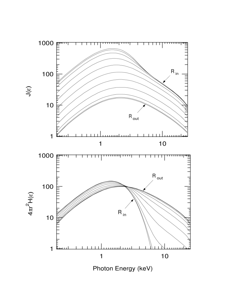
Figure 3: The zeroth and first moments of the specific intensity of the radiation field in the static, hot medium discussed in §5.1 (in arbitrary units). In both panels the curves correspond to radii in the medium that are equidistant in the parameter Q (see eq.[19]).

For the first model problem, I consider a static, spherically symmetric, purely scattering medium and set the parameters to values that are typical for weakly magnetic, accreting neutron stars (see Psaltis et al. 1995). I set the outer radius of the scattering medium to $3r_{\rm in}$, its electron temperature to 10 keV, its electron scattering optical depth to 4, and the energy-dependence of the radiation flux at the inner boundary to be that of a blackbody with a temperature of 0.5 keV; the normalization of the input flux is arbitrary because I have assumed that there are no sources of photons in the medium. This is a frequently solved problem that has been analyzed in detail by, e.g., Katz (1976), Shapiro et al. (1976), and Sunyaev & Titarchuk (1980). All these authors showed that the emerging radiation spectrum at energies much larger than the energy of the injected photons is largely independent of the details of the input spectrum and can be described by a power-law with an exponential cut-off at $\sim 3T_{e}$. Here I solve this simple problem to study the fact that the variable Eddington factors are not independent of energy even when the photon mean-free path is independent of energy and the medium is static (see also the discussion in Paper I).

Figure 3 shows the zeroth and first moments of the specific intensity of the radiation field, $J$ and $H^{r}$, as a function of photon energy and radius. Both quantities decrease overall with increasing radius because of the dilution of the radiation field. The energy dependence of the radiation energy density changes within one photon mean-free-path from the inner boundary but remains unchanged at larger radii. On the other hand, the radiation flux evolves throughout the scattering medium. This is a consequence of the fact that the system of moment equations has been solved by imposing an inner boundary condition on $H$ and an outer boundary condition on the ratio $H/J$ and not on $J$ itself.

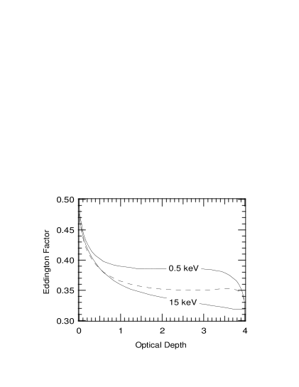
Figure 4: The first Eddington factor at two photon energies (solid lines) as well as the ratio of the energy-integrated second to zeroth moments of the specific intensity of the radiation field (dashed line) for the model problem discuss in §5.1.

Figure 4 shows the first Eddington factor $f^{rr}=K^{rr}/J$ at two photon energies as well as the ratio of the energy-integrated second to zeroth moments of the specific intensity of the radiation field. The Eddington factor depends on photon energy even though the scattering cross section and hence the photon mean-free-path are mostly energy independent at these low photon energies. This is because photons were injected into the medium with energies $\ll T_{e}$ and on average gain energy at each scattering. As a result, photons emerging with low energy have experienced on average a smaller number of scatterings than photons with higher energy and therefore their distribution is less isotropic.

Figure 5 compares the emerging radiation spectrum obtained using the method of variable Eddington factors with the spectra obtained using the same boundary conditions but two energy-independent prescriptions of the first Eddington factor that are commonly used; the second Eddington factor does not enter the calculation when the bulk velocity of the electrons is zero. Note that neither prescription is the correct diffusion approximation for Compton scattering because they both neglect the energy dependence of $f^{rr}$ on photon energy shown in Figure 4. However, the discrepancy between the self-consistent solution and the ones obtained using prescribed Eddington factors is small for the prescription that depends on optical depth and can be as large as $\sim 50$% at high photon energies for the prescription that is independent of optical depth. This discrepancy increases when the ratio of the photon mean-free path to the smallest characteristic length scale in the system increases.

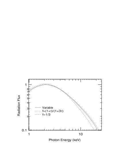
Figure 5: The radiation spectrum at the outer boundary (in arbitrary units) obtained using the method of variable Eddington factors and the spectra obtained using the same boundary conditions but two energy-independent prescriptions of the first Eddington factor.

5.2 Compton Scattering in a Divergence-Free Flow

In a moving medium, the photons gain energy by scattering off the fast moving electrons. As measured by an observer comoving with the medium, the photon energy density increases mostly due to the convergence of the flow, which is described by terms that are proportional to $\nabla\cdot\vec{V}$ (Blandford & Payne 1981). On the other hand, the flux that is measured by an observer at infinity increases because of the systematic energy exchange between photons and electrons, which is described mostly by terms that are second-order in $V$ (Psaltis & Lamb 1997).

In order to investigate the effects of Comptonization by the bulk electron flow and distinguish them from the effects of the convergence of the flow, I study in this section the photon-electron interaction and the formation of spectra in fast, divergence-free flows. For the model problems shown below, I set the outer radius of the scattering medium to $30r_{\rm in}$, the electron temperature to zero, and the electron velocity to the divergence-free profile $V=0.2r^{-2}$. Finally, I set the electron density to a constant value, which arises from mass conservation in the flow, and characterize each flow by the total electron scattering optical depth in the radial direction.

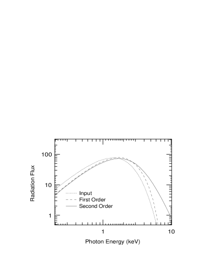
Figure 6: The radiation spectrum at the inner boundary (dotted line), the emerging radiation spectrum when only terms that are first-order in the electron bulk velocity are taken into account (dashed line), and the emerging radiation spectrum that is correct to second order in the electron bulk velocity (solid line), in arbitrary units, for the configuration discussed in §5.2.

Figure 6 shows the radiation spectrum at the inner boundary, the emerging radiation spectrum when only terms that are first-order in the electron bulk velocity are taken into account, as well as the emerging radiation spectrum that is correct to second order in the electron bulk velocity, for a flow with a scattering optical depth of 2. The terms that are first-order in the electron bulk velocity describe mainly the effects of non-relativistic Doppler shift and hence produce a displacement in $\log\epsilon$ of the input spectrum towards higher photon energies (see also Psaltis & Lamb 2000). On the other hand, the terms that are second-order in the electron bulk velocity result in a systematic photon upscattering and produce a power-law tail at photon energies higher than the average energy of the injected photons. Note here that the approximation employed here of keeping, in the scattering kernel, only terms that are first order in $\epsilon$ limits the validity of the calculation to energies $\lesssim 100$ keV.

When the total optical depth of the scattering medium, and hence the average number of scatterings that each photon experiences, are increased, then on average photons gain more energy by scattering off moving electrons. As a result, the emerging radiation spectrum is displaced towards higher photon energies, and the power-law tail becomes flatter (see Fig. 7a). When the bulk electron velocity in the flow increases, the average energy gain per scattering increases as well, and hence the power-law tail also becomes flatter (Fig. 7b). As a result, scattering of photons by fast moving electrons produces power-law tails at high photon energies, even in divergence-free flows, in a way that is similar to the well understood process of thermal Comptonization.

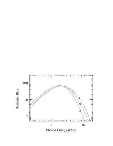
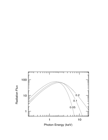
Figure 7: The dependence of the emerging radiation spectrum (in arbitrary units) on (a) the electron scattering optical depth and (b) the maximum electron bulk velocity, when the scattering optical depth is set to 5, for the configuration discussed in §5.2.

5.3 Compton Scattering in Inflows and Outflows

I finally perform simple model calculations of accretion onto and outflows from a central object by assuming a free-fall density profile and setting everywhere in the flow the electron temperature to zero and the inward radial velocity equal to the free-fall velocity from infinity onto a compact object with a radius of 10 km and a gravitational mass of $1.4M_{\odot}$. I also set the outer radius of the medium to $30r_{\rm in}$; at these large radii the photon mean-free path is large compared to radius and the electron bulk velocity is small compared to the speed of light that the flow does not effect significantly the photon distribution. Finally, instead of specifying the mass accretion rate onto the compact object, I specify the total electron-scattering optical depth of the flow.

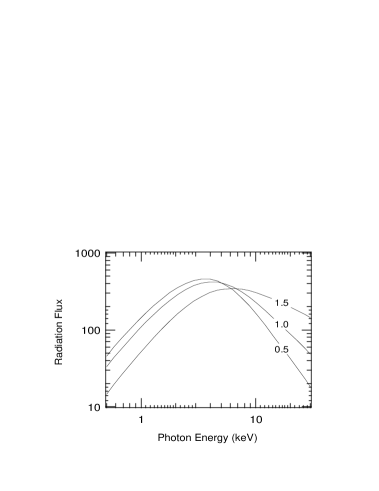
Figure 8: (a) The radiation spectrum at the inner boundary (dotted line), the emerging radiation spectrum when only terms that are first-order in the electron bulk velocity are taken into account (dashed line), and the emerging radiation spectrum that is correct to second order in the electron bulk velocity (solid line), in arbitrary units, for the inflow problem discussed in §5.3. (b) The dependence of the emerging radiation spectrum on the electron-scattering optical depth of the flow.

Figure 8a shows the radiation spectrum at the inner boundary, the emerging radiation spectrum when only terms that are first-order in the electron bulk velocity are taken into account, as well as the emerging radiation spectrum that is correct to second order in the electron bulk velocity. As in the model calculation discussed in §5.2, the terms that are first-order in the electron bulk velocity describe mostly the non-relativistic Doppler shifts and produce a displacement in $\log\epsilon$ of the input radiation spectrum towards higher photon energies. On the other hand, the terms that are second-order in the electron bulk velocity systematically upscatter photons and produce a power-law tail at high photon energies. When the optical depth of the flow is increased, the systematic upscattering of photons becomes more efficient and the high-energy tail becomes flatter.

Figure 9 shows the same information as Figure 8 but for the case of an outflow. For this model problems I have used the same parameters as in the inflow calculation but changed the sign of the velocity at all radii. In an outflow, the terms that are first-order in the electron bulk velocity produce a displacement in $\log\epsilon$ of the input radiation spectrum towards lower photon energies. On the other hand, the effect of the terms that are second-order in the electron bulk velocity is the same as in the case of inflow, i.e., they systematically upscatter the photons and produce a tail at high photon energies. For the optical depths and bulk velocities considered here, the effect of the second-order terms nearly cancels the effect of the first-order terms and the major difference between the input and emerging spectra is the power-law tail at high photon energies. As in the case of the inflow, when the optical depth of the flow increases, the power-law tail becomes flatter, but the overall effects is significantly reduced.

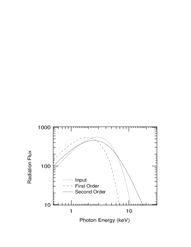
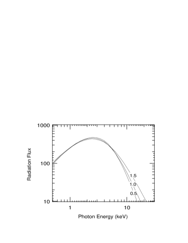
Figure 9: Same as in Figure 8, but for the outflow problem discussed in §5.3.

6 DISCUSSION

In the previous sections I described a method for solving numerically the radiative transfer equation that describes Compton scattering in spherically symmetric, static and moving media, and applied it to a variety of cases related to flows around compact objects. I showed that the first Eddington factor, which describes the degree of isotropy of the radiation field at a given point in space, may depend on photon energy, even though the photon mean-free-path is energy independent, if the photons are preferably upscattered or downscattered in energy at each scattering. I also demonstrated that the terms that are first-order in the electron bulk velocity alter the input spectrum in a way that is qualitatively and quantitatively different than the effect of the terms that are of second-order.

The systematic upscattering of photons caused by bulk Comptonization is described by the terms that are second-order in $V$. This becomes apparent by the fact that, at each scattering with a moving electron, the average fractional energy change of a photon in the system frame is always positive, independent of the photon energy, and equal to $4V^{2}/3$ (see, e.g., Rybicki & Lightman 1979, ch. 7; see also the discussion in Psaltis & Lamb 1997). If the distribution of photon residence times in the Comptonizing medium drops exponentially to zero at late times, then a power-law tail is produced at high photon energies (for total scattering optical depths $\gtrsim 1$), in analogy to the generation of power-law tails by thermal Comptonization. The velocity at which the terms that are second-order in $V$ become important depends on the ratio of the photon mean-free-path $\lambda_{\rm mfp}$ to the shortest characteristic length scale $L$ in the problem. In general, when $V(L/\lambda_{\rm mfp})\sim 1$, i.e., in regions close to and within the photon-trapping radius, the terms that are first- and second-order in $V$ become comparable in size (Yin & Miller 1995; Psaltis & Lamb 1997a) and hence the latter should not be neglected.

The generalization of the method to time-independent multi-dimensional configurations is conceptually easy. However, a problem with axial symmetry requires the solution of the radiative transfer equation in five dimensions in phase space and the introduction of a large number of independent variable Eddington factors. Moreover, the presence of high flow velocities in multi-dimensions introduces sharp gradients in the variable Eddington factors, which cannot be guessed a priori, as required for the first iteration (Dykema, Klein, & Castor 1996). Even with these problems, however, the method of variable Eddington factors will still offer a significant advantage, when compared to any other iterative method, which arises from the fact that the Eddington factors are bound to lie over a very narrow range of values.

The fast convergence of the numerical algorithm presented here makes it also ideal for future extensions to transport problems coupled to time-dependent hydrodynamics. For the case of accretion onto and outflows from compact objects, the characteristic photon diffusion timescale from a flow of dimension $R$ is of order

$$t_{\rm dif}\simeq\frac{R\tau}{c}=30\left(\frac{R}{10^{6}~{}\mbox{cm}}\right)\left(\frac{\tau}{1}\right)~{}\mu\mbox{s}\;,$$ (50)

which is significantly smaller than the corresponding $t_{\rm dyn}\sim 1$ ms dynamical timescale. As a result, for most cases the structure of the radiation field can be obtained by solving the time-independent radiative transfer problem for each snapshot of the fluid properties. Given that the variable Eddington factors will be only marginally different between successive timesteps, the convergence of the algorithm will be even faster than what is shown in Figure 2.

Appendix A Moments of the Specific Intensity in Spherical Geometry

In defining the moments of the specific intensity in the system frame I shall use the quantities

$$u(z,p,\epsilon)\equiv\frac{1}{2}\left[I^{+}(z,p,\epsilon)+I^{-}(z,p,\epsilon)\right]$$ (A1)

and

$$v(z,p,\epsilon)\equiv\frac{1}{2}\left[I^{+}(z,p,\epsilon)-I^{-}(z,p,\epsilon)\right]\;.$$ (A2)

The zeroth moment of the specific intensity is then

$$J(r,\epsilon)=\frac{1}{r}\int_{0}^{r}u(z,p,\epsilon)dz\;,$$ (A3)

where $r$ depends on $z$ and $p$ through the relation $r^{2}=z^{2}+p^{2}$. Because of the assumed spherical symmetry, the only non-zero component of the first moment of the specific intensity is the $r$–component:

$$H^{r}(r,\epsilon)=\frac{1}{r^{2}}\int_{0}^{r}zv(z,p,\epsilon)dz\;.$$ (A4)

Similarly, the non-zero components of the second, third, and fourth moments of the specific intensity are

$$K^{rr}(r,\epsilon) = \frac{1}{r^{3}}\int_{0}^{r}z^{2}u(z,p,\epsilon)dz$$

$$K^{\theta\theta}(r,\epsilon)=K^{\phi\phi}(r,\epsilon) = \frac{1}{2}\left(J-K^{rr}\right)\;,$$ (A5)

$$Q^{rrr}(r,\epsilon) = \frac{1}{r^{4}}\int_{0}^{r}z^{3}v(z,p,\epsilon)dz$$

$$Q^{\theta\theta r}(r,\epsilon)=Q^{\theta r\theta}(r,\epsilon)=Q^{r\theta\theta}(r,\epsilon) = \frac{1}{2}\left(H^{r}-Q^{rrr}\right)$$

$$Q^{\phi\phi r}(r,\epsilon)=Q^{\phi r\phi}(r,\epsilon)=Q^{r\phi\phi}(r,\epsilon) = \frac{1}{2}\left(H^{r}-Q^{rrr}\right)\;,$$

$$R^{rrrr}(r,\epsilon) = \frac{1}{r^{5}}\int_{0}^{r}z^{4}u(z,p,\epsilon)dz$$

$$R^{\theta\theta\theta\theta}(r,\epsilon) = \frac{3}{8}\left(J-2K^{rr}+R^{rrrr}\right)$$

$$R^{\phi\phi\phi\phi}(r,\epsilon) = \frac{3}{8}\left(J-2K^{rr}+R^{rrrr}\right)$$

$$R^{rr\theta\theta}(r,\epsilon)=R^{r\theta r\theta}(r,\epsilon)=... = \frac{1}{2}\left(K^{rr}-R^{rrrr}\right)$$

$$R^{rr\phi\phi}(r,\epsilon)=R^{r\phi r\phi}(r,\epsilon)=... = \frac{1}{2}\left(K^{rr}-R^{rrrr}\right)$$

$$R^{\theta\theta\phi\phi}(r,\epsilon)=R^{\theta\phi\theta\phi}(r,\epsilon)=... = \frac{3}{8}R^{rrrr}\;.$$ (A6)

Finally, I shall also use the first two Eddington factors defined by

$$f^{rr} \equiv \frac{K^{rr}}{J}$$ (A7)

$$g^{rr} \equiv \frac{Q^{rrr}}{H^{r}}\;.$$ (A8)

Appendix B The Generalized Source Function

Using equation (A8)–(A12) of Paper I, I derive the generalized source function for a spherically symmetric system:

$$S^{\pm}(z,p,\epsilon)\equiv S_{1}^{\pm}+\epsilon S_{2}^{\pm}+T_{e}S_{3}^{\pm}+VS_{4}^{\pm}+V^{2}S_{5}^{\pm}\;,$$ (B1)

where

$$S_{1}^{\pm} = \frac{3}{8}\left[3-\cos^{2}\theta+\left(3\cos^{2}\theta-1\right)f^{rr}\right]J$$ (B2)

$$S_{2}^{\pm} = \frac{3}{8}\left\{\left(-1+\epsilon\partial_{\epsilon}\right)\left[3-\cos^{2}\theta+\left(3\cos^{2}\theta-1\right)f^{rr}\right]\right.J$$ (B3)

$$\quad\quad+\left.\left(1-\epsilon\partial_{\epsilon}\right)\left[5-3\cos^{2}\theta+\left(5\cos^{2}\theta-3\right)g^{rr}\right]H^{r}\cos\theta\right\}$$

$$S_{3}^{\pm} = \frac{3}{4}\left\{\left[3\cos^{2}\theta-1-3\left(3\cos^{2}\theta-1\right)f^{rr}\right]J\right.$$ (B4)

$$\quad\quad+2\left[1-3g^{rr}+\left(5g^{rr}-3\right)\cos^{2}\theta\right]H^{r}\cos\theta$$

$$\quad\quad+\frac{1}{2}\left(-2\epsilon\partial_{\epsilon}+\epsilon^{2}\partial^{2}_{\epsilon}\right)\left[3-\cos^{2}\theta+\left(3\cos^{2}\theta-1\right)f^{rr}\right]J$$

$$\quad\quad+\frac{1}{2}\left(2\epsilon\partial_{\epsilon}-\epsilon^{2}\partial^{2}_{\epsilon}\right)\left[5-3\cos^{2}\theta+\left(5\cos^{2}\theta-3\right)g^{rr}\right]H^{r}\cos\theta$$

$$S_{4}^{\pm} = V\cos\theta I+\frac{3}{8}V\left\{4\cos\theta\left[2-\cos^{2}\theta+\left(3\cos^{2}\theta-2\right)f^{rr}\right]J\right.$$ (B5)

$$\quad\quad+\left[-1-5\cos^{2}\theta+\left(3\cos^{2}\theta-1\right)g^{rr}\right]H^{r}$$

$$\quad\quad-\cos\theta\partial_{\epsilon}\left[3-\cos^{2}\theta+\left(3\cos^{2}\theta-1\right)f^{rr}\right]J$$

$$\quad\quad\left.+\partial_{\epsilon}\left[\frac{1}{2}\left(3-\cos^{2}\theta\right)+\left(3\cos^{2}\theta-1\right)g^{rr}\right]H^{r}\right\}$$

$$S_{5}^{\pm} = \frac{3}{4}V^{2}\left\{\left[-5\cos^{4}\theta+\frac{21}{2}\cos^{2}\theta-1-2\cos^{2}\theta\left(2-\cos^{2}\theta\right)\epsilon\partial_{\epsilon}\right.\right.$$ (B6)

$$\quad\quad\quad\quad\left.+\frac{1}{4}\cos^{2}\theta\left(3-\cos^{2}\theta\right)\epsilon^{2}\partial_{\epsilon}^{2}\right]J$$

$$\quad\quad+\left[4-10\cos^{2}\theta+\left(3+\cos^{2}\theta\right)\epsilon\partial_{\epsilon}-\frac{1}{2}\left(3-\cos^{2}\theta\right)\epsilon^{2}\partial_{\epsilon}^{2}\right]\cos\theta H$$

$$\quad\quad+\left[\frac{1}{2}\left(30\cos^{4}\theta-37\cos^{2}\theta+7\right)+2\left(1-3\cos^{4}\theta\right)\epsilon\partial_{\epsilon}\right.$$

$$\quad\quad\quad\quad\left.+\frac{1}{4}\left(3\cos^{4}\theta-3\cos^{2}\theta+4\right)\epsilon^{2}\partial_{\epsilon}^{2}\right]f^{rr}K^{rr}$$

$$\quad\quad+\left[\left(6\cos^{2}\theta-4\right)+\left(3\cos^{2}\theta-3\right)\epsilon\partial_{\epsilon}-\frac{1}{2}\left(3\cos^{2}\theta-1\right)\epsilon^{2}\partial_{\epsilon}^{2}\right]\cos\theta g^{rr}H^{r}$$

$$\quad\quad\left.+\left(2\cos^{2}\theta-1\right)\left(1+2\epsilon\partial_{\epsilon}+\frac{1}{2}\epsilon^{2}\partial_{\epsilon}^{2}\right)R^{rrrr}\right\}$$

where $cos\theta\equiv z/r$ and the variable Eddington factors and the moments of the specific intensity are defined as in Appendix A.

Appendix C Coefficients of the Moment Equations

Using equations (34) and (40) of Paper I, I derive

$$A_{1} = n_{e}\left[\epsilon+V^{2}\left(\frac{1}{10}\epsilon\partial_{\epsilon}+\frac{11}{20}\epsilon^{2}\partial^{2}_{\epsilon}\right)f^{rr}\right]$$ (C1)

$$\quad\quad-\left[1+\frac{1}{2}V^{2}+\left(f^{rr}+\frac{1}{2}\right)V^{2}\epsilon\partial_{\epsilon}+\frac{1}{2}f^{rr}V^{2}\epsilon^{2}\partial^{2}_{\epsilon}\right]\chi$$

$$A_{2} = n_{e}\left\{\epsilon-2T_{e}-\frac{2}{3}V^{2}+\left[\frac{1}{10}\left(f^{rr}-\frac{1}{3}\right)+\frac{22}{20}\epsilon\partial_{\epsilon}f^{rr}\right]V^{2}\right\}$$ (C2)

$$A_{3} = n_{e}\left[T_{e}+\frac{1}{3}V^{2}+\frac{11}{20}\left(f^{rr}-\frac{1}{3}\right)V^{2}\right]$$ (C3)

$$A_{4} = -\frac{2}{\tau_{0}-\tau_{\rm r}}+V\chi+V\epsilon\partial_{\epsilon}\chi$$ (C4)

$$A_{5} = n_{e}V$$ (C5)

$$C_{1} = -\chi S_{e}+\frac{1}{6}V^{2}S_{e}\left(\epsilon\partial_{\epsilon}-\epsilon^{2}\partial^{2}_{\epsilon}\right)\chi+\frac{1}{6}V^{2}\epsilon\left(\partial_{\epsilon}S_{e}\right)\left(1-2\epsilon\partial_{\epsilon}\right)\chi$$ (C6)

$$-\frac{1}{6}V^{2}\epsilon^{2}\left(\partial^{2}_{\epsilon}S_{e}\right)\chi$$

and

$$B_{1} = \frac{1}{10}n_{e}V\left(9f^{rr}-7-\epsilon\partial_{\epsilon}f^{rr}\right)+Vf^{rr}\left(1+\epsilon\partial_{\epsilon}\right)\chi$$ (C7)

$$\quad\quad+\partial_{\tau_{r}}f^{rr}-\frac{3}{\tau_{0}-\tau_{\rm r}}\left(f^{rr}-\frac{1}{3}\right)$$

$$B_{2} = -\frac{1}{10}n_{e}V\left(f^{rr}+3\right)$$ (C8)

$$B_{3} = n_{e}\left[-1+\frac{12}{5}\epsilon-\frac{2}{5}T_{e}-\frac{1}{2}V^{2}+\frac{1}{10}V^{2}\left(-1-3\epsilon\partial_{\epsilon}-\partial^{2}_{\epsilon}\right)g^{rr}\right]$$ (C9)

$$\quad\quad-\left[1+\frac{1}{2}V^{2}+V^{2}\left(g^{rr}+\frac{1}{2}\right)\epsilon\partial_{\epsilon}+\frac{1}{2}V^{2}g^{rr}\epsilon^{2}\partial^{2}_{\epsilon}\right]\chi$$

$$B_{4} = n_{e}\left[-\frac{2}{5}\epsilon+\frac{4}{5}T_{e}+\frac{9}{10}V^{2}-\frac{3}{10}V^{2}\left(1+\frac{2}{3}\epsilon\partial_{\epsilon}\right)g^{rr}\right]$$ (C10)

$$B_{5} = n_{e}\left[-\frac{2}{5}T_{e}-\frac{1}{10}V^{2}\left(g^{rr}+3\right)\right]$$ (C11)

$$C_{2} = -\frac{2}{3}V\chi S_{e}+\frac{1}{3}V\chi\epsilon\partial_{\epsilon}S_{e}+\frac{1}{3}VS_{e}\epsilon\partial_{\epsilon}\chi\;,$$ (C12)

where $\tau_{0}\equiv\tau_{\rm r}(r=r_{\rm in})$ and I have suppressed the dependence of the various quantities on spatial position and photon energy.

Appendix D Coefficients for Differencing the Moment Equations

Using equations (34) and (40) of Paper I I derive

$$A_{1}^{\prime} = n_{e}V^{2}\left(\frac{1}{10}\epsilon\partial_{\epsilon}+\frac{11}{20}\epsilon^{2}\partial^{2}_{\epsilon}\right)f^{rr}$$ (D1)

$$\quad\quad-\left[1+\frac{1}{2}V^{2}+\left(f^{rr}+\frac{1}{2}\right)V^{2}\epsilon\partial_{\epsilon}+\frac{1}{2}f^{rr}V^{2}\epsilon^{2}\partial^{2}_{\epsilon}\right]\chi$$

$$A_{2}^{\prime} = n_{e}\left[\frac{1}{10}\left(f^{rr}-\frac{1}{3}\right)+\frac{22}{20}\epsilon\partial_{\epsilon}f^{rr}\right]V^{2}$$ (D2)

$$A_{3}^{\prime} = n_{e}\frac{11}{20}\left(f^{rr}-\frac{1}{3}\right)V^{2}$$ (D3)

$$A_{4}^{\prime} = -\frac{2}{\tau_{0}-\tau_{\rm r}}+V\chi+V\epsilon\partial_{\epsilon}\chi$$ (D4)

$$C_{1}^{\prime} = -\chi S_{e}+\frac{1}{6}V^{2}S_{e}\left(\epsilon\partial_{\epsilon}-\epsilon^{2}\partial^{2}_{\epsilon}\right)\chi+\frac{1}{6}V^{2}\epsilon\left(\partial_{\epsilon}S_{e}\right)\left(1-2\epsilon\partial_{\epsilon}\right)\chi$$ (D5)

$$-\frac{1}{6}V^{2}\epsilon^{2}\left(\partial^{2}_{\epsilon}S_{e}\right)\chi\;,$$

where $\tau_{0}\equiv\tau_{\rm r}(r=r_{\rm in})$ and I have suppressed the dependence of the various quantities on spatial position and photon energy.

References

- (1)
- (2) Ames, W. F. 1992, Numerical Methods for Partial Differential Equations, (Boston: Academic Press, Inc)
- (3)
- (4) Burrows, A., Young, T., Pinto, P. A., Eastman, R., & Thompson, T. 2000, ApJ, in press (astro-ph/9905132)
- (5)
- (6) Babuel-Peyrissac, J. P. & Rouvillois, G. 1969, J. Phys., 30, 301
- (7)
- (8) Blandford, R. D. & Payne, D. G. 1981a, MNRAS, 194, 1033
- (9)
- (10) ——–. 1981b, MNRAS, 194, 1040
- (11)
- (12) Chan, K. L. & Jones, B. J. T. 1975, ApJ, 200, 454
- (13)
- (14) Chang, J. S., & Cooper, G. 1970, 6, 1
- (15)
- (16) Colpi, M. 1988, ApJ, 326, 233
- (17)
- (18) Dykema, P. G., Klein, R. I., & Castor, J. I. 1996, ApJ, 457, 892
- (19)
- (20) Esin, A., McClintock, J. E., & Narayan, R. 1997, ApJ, 289, 865
- (21)
- (22) Fukue, J., Kato, S., & Matsumoto, R. 1985, PASJ, 37, 383
- (23)
- (24) Hsu, C.-M., & Blaes, O. 1998, ApJ, 506, 658
- (25)
- (26) Katz, J. I. 1987, High Energy Astrophysics (Menlo Park, CA: Addison-Wesley)
- (27)
- (28) Kompaneets, A. S. 1957, Sov. Phys. JETP, 4, 730
- (29)
- (30) Körner, A., & Janka, H.-Th. 1992, A&A, 266, 613
- (31)
- (32) Laurent, P., & Titarchuk, L. 1999, ApJ, 511, 289
- (33)
- (34) Lindquist, R. W. 1966, Ann. Phys., 37, 487
- (35)
- (36) Lyubarskij, Y. E. & Sunyaev, R. A. 1982, Sov. Astr. Let., 8, 330
- (37)
- (38) Madej, J. 1989, ApJ, 339, 386
- (39)
- (40) ——–. 1991, ApJ, 376, 161
- (41)
- (42) Mastichiadis, A. & Kylafis, N. D. 1992, ApJ, 384, 136
- (43)
- (44) Mihalas, D. 1978, Stellar Atmospheres (New York: W.H. Freeman & Co.)
- (45)
- (46) ——–. 1980, ApJ, 238, 1034
- (47)
- (48) Papathanassiou, H., & Psaltis, D. 2000, MNRAS, submitted
- (49)
- (50) Payne, D. G. 1980, ApJ, 237, 951
- (51)
- (52) Payne, D. G. & Blandford, R. D. 1981, MNRAS, 196, 781
- (53)
- (54) Pomraning, G. C. 1973, The Equations of Radiation Hydrodynamics, International Series of Monographs in Natural Philosophy, Vol. 54 (Oxford: Pergamon Press)
- (55)
- (56) Poutanen, J., & Svensson, R. 1996, ApJ, 470, 249
- (57)
- (58) Pozdnyakov, L. A., Sobol, I. M., & Sunyaev, R. A. 1983, Astr. Sp. Phys. Rev., 2, 189
- (59)
- (60) Press, W. H., Teukolsky, S. A., Vetterling, W. T., Flannery, B. P. 1992, Numerical Recipes in Fortran (Cambridge: University Press)
- (61)
- (62) Psaltis, D. 1998, Ph. D. Thesis, University of Illinois, Urbana-Champaign
- (63)
- (64) Psaltis, D., & Lamb, F. K. 1997, ApJ, 488, 881 (Paper I)
- (65)
- (66) ———. 2000, ApJ, submitted
- (67)
- (68) Psaltis, D., Lamb, F. K., & Miller, G. S. 1995, ApJ, 454, L137
- (69)
- (70) Riffert, H. 1988, ApJ, 327, 760
- (71)
- (72) Rybicki, G. B. & Lightman, A. L. 1979, Radiative Processes in Astrophysics (New York: John Wiley)
- (73)
- (74) Schmid-Burgk, J. 1978, Astr. Sp. Sc., 56, 191
- (75)
- (76) Shapiro, S. L., Lightman, A. P., & Eardly, D. M. 1976, ApJ, 204, 187
- (77)
- (78) Smit, J. M., Cernohorsky, J., & Dullemond, C. P. 1997, A&A, 325, 203
- (79)
- (80) Sunyaev, R. A. & Titarchuk, L. G. 1980, A&A 86, 121
- (81)
- (82) Sunyaev, R. A. & Zeldovich, Ya. B. 1980, ARAA, 18, 537
- (83)
- (84) Thorne, K. S. 1981, MNRAS, 194, 439
- (85)
- (86) Titarchuk, L. 1994, ApJ, 434, 570
- (87)
- (88) Titarchuk, L. & Lyubarskij, Y. E. 1995, ApJ, 450, 876
- (89)
- (90) Titarchuk, L., Mastichiadis, A., & Kylafis, N. D. 1997, ApJ, 487, 834
- (91)
- (92) Titarchuk, L., Zannias, T., 1998, ApJ, 493, 863
- (93)
- (94) Turolla, R., Zampieri, L., & Nobili, L. 1995, MNRAS, 272, 625
- (95)
- (96) Turolla, R., Zane, S., Zampieri, L., & Nobili, L. 1996, MNRAS, 283, 881
- (97)
- (98) Yin, W.-W. & Miller, G. S. 1995, ApJ, 449, 826
- (99)
- (100) Zampieri, L., Turolla, R., Zane, S., & Treves, A. 1995, ApJ, 439, 849
- (101)
- (102) Zane, S., Turolla, R., Nobili, L., & Erna, M. 1996, ApJ, 466, 871
- (103)