Extended quintessence and the primordial helium abundance

Abstract

In extended quintessence models, a scalar field which couples to the curvature scalar $R$ provides most of the energy density of the universe. We point out that such models can also lead naturally to a decrease in the primordial abundance of helium-4, relieving the tension which currently exists between the primordial helium-4 abundance inferred from observations and the amount predicted by Standard Big Bang Nucleosynthesis (SBBN) corresponding to the observed deuterium abundance. Using negative power-law potentials for the quintessence field, we determine the range of model parameters which can lead to an interesting reduction in the helium-4 abundance, and we show that it overlaps with the region allowed by other constraints on extended quintessence models.

]

I Introduction

A great deal of observational evidence currently points toward a cosmological model with a nonzero cosmological constant $\Lambda$. A combination of the supernova Ia measurements [4], measurements of the baryon fraction in galaxy clusters [5], and the location of the first acoustic peak of the microwave background anisotropies [6] suggests a model with $\Omega_{{\rm M}}=0.3-0.4$ and $\Omega_{\Lambda}=0.6-0.7$.

A genuine cosmological constant is a disaster from the standpoint of particle physics, in which the most natural value of $\Lambda$ is many orders of magnitude larger than the “observed” value (see Ref. [7] for a review). However, even if a plausible particle physics mechanism were developed to produce such a small value of $\Lambda$, a second problem remains: why are $\Omega_{\Lambda}$ and $\Omega_{{\rm M}}$ comparable today? Since $\Omega_{\Lambda}$ and $\Omega_{{\rm M}}$ scale very differently with the cosmological expansion factor, this coincidence suggests that we live in a very special epoch. This problem has been dubbed the “cosmological constant coincidence problem” to distinguish it from the more fundamental cosmological constant problem [8, 9].

A possible solution to the coincidence problem is to assume that the apparent cosmological constant is not, in fact, a true constant vacuum energy density, but instead is due to the energy density of a scalar field $\phi$, a possibility which has come to be known as quintessence. It might then be possible to couple the behavior of this field to the background matter density in such way as to achieve ‘naturally’ the desired result, namely $\Omega_{\phi}\approx\Omega_{{\rm M}}$ today. Of course, in this case, the scalar field may have an equation of state intermediate between matter and a cosmological constant. This possibility was explored in some detail by Zlatev et al. [8] (see also reference [9]) who argued that a certain class of solutions (“tracking solutions”) will evolve toward the desired behavior independent of the initial conditions. Although such models still require fine tuning to produce $\Omega_{\phi}\approx\Omega_{{\rm M}}$ today [10], they seem to be pointing in a more plausible direction toward this result.

These investigations assumed minimally-coupled scalar fields, but it was soon realized that coupling the scalar field to the curvature scalar $R$ opens up another range of possibilities, dubbed “extended quintessence.” Uzan [11] examined the general case of a non-minimally coupled scalar field evolving in an exponential or power-law potential, and Amendola [12] explored a general class of couplings and potentials. Non-minimally coupled models suffer from the potential problem that the gravitational constant $G$ varies in time [12, 13], but they have nonetheless received a great deal of recent attention as possible models for quintessence [14] - [16].

In this paper, we point out an interesting consequence of non-minimally coupled quintessence models: under some circumstances these models can lead to a reduction in the primordial helium abundance. This is of interest because of a “tension” between the recent estimate of the primordial deuterium abundance, $D/H=3.0\pm 0.4\times 10^{-5}$ [17], which leads to an estimate for the baryon/photon ratio of $\eta=5.6\pm 0.5\times 10^{-10}$, and the corresponding SBBN predicted primordial helium-4 abundance of $Y_{P}=0.248\pm 0.001$. In contrast, the actual primordial helium abundance is likely lower. For example, Olive and Steigman found [18]

$$Y_{P}=0.234\pm 0.003({\rm stat.}),$$ (1)

while Izotov and Thuan obtained a higher value [19]

$$Y_{P}=0.244\pm 0.002({\rm stat.}).$$ (2)

While this apparent discrepancy is insufficient to discard SBBN, it certainly represents a “tension” in the model. Furthermore, in addition to the three standard model neutrinos, a sterile neutrino may be needed to explain the results from neutrino oscillation experiments [20]. If either or both of these were confirmed, or if there are any other light particles in the Universe, the breach between theory and observation on $~{}^{4}\mathrm{He}$ could become even wider.

In light of these SBBN results, any “natural” mechanism which lowers the primordial helium-4 abundance must be regarded as interesting. In this paper we show that extended quintessence models provide just such a mechanism. In Ref. [14], Perrotta et al. investigated the BBN constraint on the extended quintessence model. They showed that the model is not ruled out by increasing helium, but they did not consider the more interesting possibility of decreasing helium.

In the next section, we review the evolution of the scalar field in these models and calculate the reduction in the abundance of helium-4 as a function of the model parameters. We determine whether an interesting reduction is consistent with other constraints on extended quintessence. Our results are summarized in Sec. 3. We shall use units in which $\hbar=c=8\pi G_{N}=1$ throughout, unless otherwise stated.

II The Non-Minimally Coupled Quintessence model

The action for an extended quintessence model is given by [11, 14]

$$S=\int d^{4}x\sqrt{-g}\left[f(R,Q)-\frac{1}{2}\omega(Q)Q^{;\mu}Q_{;\mu}-V(Q)+L_{\rm fluid}\right],$$ (3)

where $R$ is the curvature scalar of the space-time and $Q$ is a scalar field. We adopt the Non-Minimally Coupled (NMC) model of Refs. [14, 16], in which $\omega(Q)=1$, $f(Q,R)=\frac{1}{2}F(Q)R$, and $F(Q)$ takes the form,

$$F(Q)=1-\xi(Q^{2}-Q_{0}^{2}),\quad$$ (4)

where $Q_{0}$ is the value of $Q$ today. (The zero subscript will refer throughout to quantities evaluated at the present). Eq. (4) ensures that $F(Q)=1$ today.

The coupling constant $\xi$ in the NMC quintessence model is constrained by solar system limits on $\omega_{JBD}$, the Jordan-Brans-Dicke parameter [14]:

$$\omega_{JBD}=\frac{F_{0}}{(\partial F/\partial Q)_{0}^{2}}>500,$$ (5)

as well as the experimental limit on variation of the gravitational constant [14]:

$$|\dot{G}/G|_{0}=|\dot{F}/F|_{0}<10^{-11}{\rm yr}^{-1}.$$ (6)

Using the form for $F(Q)$ from Eq. (4), these limits translate into:

$$\xi Q_{0}<0.022,$$ (7)

from the solar system constraint, and

$$2\xi Q_{0}\dot{Q}_{0}<10^{-11}{\rm yr}^{-1},$$ (8)

from the limits on the time variation of $G$.

In this model, the expansion rate of the Universe is

$$H^{2}=\frac{1}{3F}\left(\rho_{f}+\frac{1}{2}\dot{Q}^{2}+V(Q)+6H\xi Q\dot{Q}\right),$$ (9)

where $\rho_{f}=\rho_{m}+\rho_{r}$ is the density contribution from matter and radiation (including neutrinos). The evolution of $Q$ is governed by

$$\ddot{Q}+3H\dot{Q}+{\partial V\over\partial Q}+\xi RQ=0.$$ (10)

The scalar curvature is given by

$$R = 6(\dot{H}+2H^{2})$$ (11)

$$= \frac{1}{F}\left(\rho_{f}-3p_{f}-\dot{Q}^{2}+4V+6\xi(\dot{Q}^{2}+Q\ddot{Q}+3HQ\dot{Q})\right).$$ (12)

As a specific case, we will consider the inverse power law potential for $Q$:

$$V(Q)=V_{0}Q^{-\alpha}.$$ (13)

However, our final results can be generalized to other forms for the potential. It is known that with this type of potential, the quintessence energy redshifts more slowly than the radiation in the radiation-dominated era, and more slowly than the matter in the matter-dominated era, ultimately dominating at late times [8, 9, 10, 16, 21], thus providing an explanation for the observed accelerating expansion of the Universe [4]. The vacuum energy observed today is determined by $V_{0}$ but is not (or is only weakly) dependent on the initial value of $Q$, thus, partly addressing the “fine tuning problem” [8, 9].

FIG. 1.: The evolution of $Q$ for a potential $V=V_{0}Q^{-4}$, where $V_{0}$ is chosen to satisfy the boundary conditions given in equations (15), and $\xi=0.007$.

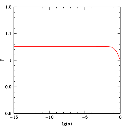
FIG. 2.: As in Fig. 1, for the evolution of $F$.

A viable NMC cosmological model must satisfy the following boundary conditions at $a=1$:

• The effective gravitational constant today must be equal to the measured value, which translates to the requirement

  $$F|_{a=1}=1.$$ (14)

  This condition is satisfied automatically by our definition in equation (4).

• After evolving the model from an early epoch to the present one, we must recover the present value of cosmological parameters, which we take to be:

  $$\Omega_{M0}=0.3,\qquad H_{0}=65~{}{\rm km/sec/Mpc}$$ (15)

where, as noted above, we take $\Omega_{0}=1$. As an example, we show the evolution of $Q$, $F$, and the densities of interest which satisfy our boundary conditions in Figs. 1-3, for the case $V=V_{0}Q^{-4}$, $\xi=0.007$.

The general behavior of the NMC quintessence model with this potential was discussed in Ref. [16]; here we review it briefly. At sufficiently early times, the $\xi RQ$ term in equation (10) dominates the $\partial V/\partial Q$ term, and the field $Q$ settles down to a slow roll regime, with an effective potential $\xi RQ$ balanced by a “frictional force” $-3H\dot{Q}$. (This dominance of the $\xi RQ$ term has been dubbed the “R-boost” [16]). In this regime, $Q$ is nearly constant (as seen in Fig. 1), and the potential term $V$ is sub-dominant; $V$ affects neither the expansion nor the $Q$-evolution significantly. The slow roll holds until $V$ becomes significant, after which $Q$ begins to roll fast, and the quintessence kinetic and potential energy come to dominate. In this regime, the $\xi RQ$ term can be neglected, and the field behaves as a minimally coupled “tracker” field with a negative power law potential [8, 9, 10, 16, 21]. The results we show in Figs. 1-3 are in agreement with those of Ref. [16].

Depending on the choice of the initial conditions, the history of the $Q$ field may have a few more twists than described above; we refer the reader to Ref. [16] for more details. For our purpose, it is sufficient to note that the early slow roll and the late tracker behavior are common features for most of these models, and we will confine our investigation to the range of parameters for which this behavior holds.

FIG. 3.: As in Fig. 1, for the evolution of the fluid and Q-field energy densities.

Our model appears to have four free parameters: $V_{0}$, $\alpha$, $\xi$, and $Q_{i}$ (the initial value of $Q$), which together determine $Q_{0}$. Note, however, that $Q_{0}$ is almost completely independent of $Q_{i}$, as a consequence of the tracker behavior of the model [8, 9]. This is displayed in Fig. 4

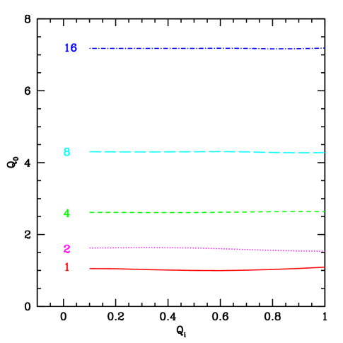
FIG. 4.: $Q_{0}$ as a function of $Q_{i}$ for various values of $\alpha$, shown on the left side of each curve, for $\xi=0.02$.

Hence, $Q_{0}$ is effectively only a function of $\alpha$, $V_{0}$, and $\xi$. However, once we fix $\alpha$, and $\xi$, the value of $V_{0}$ is fixed by boundary conditions of Eq. (15). So effectively, $\alpha$ and $\xi$, along with the boundary conditions, fix $Q_{0}$. This dependence is shown in Fig. 5. It is obvious from this figure that $Q_{0}$ is also nearly independent of $\xi$. This follows from the fact that the term containing $\xi$ in Eq. (10) is subdominant once tracking behavior starts. Hence, it is a good approximation to take $Q_{0}$ to be a function of $\alpha$ alone for boundary conditions fixed as in Eq. (15).

Since the solar system limit (Eq. 7) is a constraint on $\xi$ and $Q_{0}$, it translates into a constraint on $\xi$ for a given value of $\alpha$. This limit is shown in Fig. 6. For the models we consider here, the limit from equation (8) is subdominant and can be ignored.

FIG. 5.: $Q_{0}$ as a function of $\alpha$, for (from top to bottom) $\xi=0.002,0.004,0.008,0.012,0.016,0.02$.

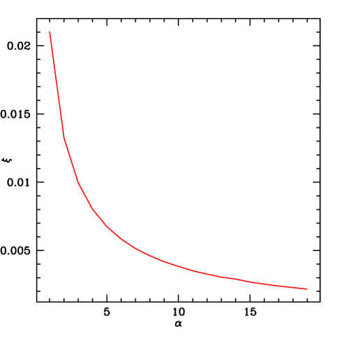
FIG. 6.: The strongest coupling for a given $\alpha$ allowed by solar system experiments.

Now consider the effect on the expansion rate. Let $H$ be the Hubble parameter in our NMC quintessence model, and let $\bar{H}$ be the Hubble parameter in a fiducial (no quintessence) model, which we take to be a standard $\Lambda$CDM model with $\Omega_{\Lambda}=0.7$, $\Omega_{0}=1$. (Our specific choice of fiducial model is relevant only at late times and does not affect our BBN calculations, but we choose this particular model for definiteness). In order to reduce the helium abundance, we would like $H<\bar{H}$, which implies $F>1$, during BBN. However, when $V$ dominates, $Q$ rolls “down hill” in the positive direction (assume $Q>0$), so $Q_{0}>Q_{BBN}$. Therefore, we find $F>1$ if and only if $\xi>0$.

The change in expansion rate can be parametrized by a speed-up factor $\zeta$:

$$\zeta\equiv\frac{H}{\bar{H}}.$$ (16)

The evolution of $\zeta-1$ in the model of Figs. 1-3 is shown in Fig. 7. The region at the right side of the graph for which $\zeta-1>0$ arises after the quintessence field enters the tracker regime; in this regime the scaling of $\rho_{Q}$ with $a$ is different than the scaling of $\rho_{\Lambda}$ in our fiducial model. This behavior is, however, irrelevant for BBN; the value of $\zeta-1$ during BBN depends only on the radiation content of our fiducial model.

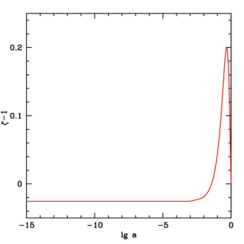
FIG. 7.: As in Fig. 1, for the evolution of the speed-up factor $\zeta$.

During BBN, $\rho_{f}$ dominates the density in equation (9), so the speed-up factor is determined primarily by the effective gravitational constant $F$. Since the $Q$ field is almost frozen during the radiation dominated era, we have $Q\approx Q_{i}$, so

$$\zeta-1\approx-{1\over 2}(F-1)\approx{1\over 2}\xi(Q_{i}^{2}-Q_{0}^{2}),$$ (17)

for $\zeta-1\ll 1$. We are primarily interested in the case $Q_{i}<<Q_{0}$, because it is in this regime one expect a large negative $\zeta-1$. In this case, we get

$$\zeta-1\approx-{1\over 2}\xi Q_{0}^{2}.$$ (18)

As we have seen, $Q_{0}$ is effectively only a function of $\alpha$, with a slight residual dependence on $\xi$ for the boundary conditions fixed in Eq. (15). Hence, the speed-up factor will be a function of $\xi$ and $Q_{0}$ alone; we expect $\zeta-1\propto\xi$ from Eq. (18), and Fig. 5 shows that $Q_{0}$, and hence the magnitude of $\zeta-1$ should increase with increasing $\alpha$. The dependence of $\zeta-1$ as a function of $\xi$ and $\alpha$ is shown in Fig. 8.

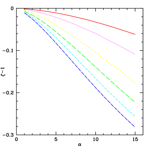
FIG. 8.: The value of $\zeta-1$ during nucleosynthesis as a function of $\alpha$; the five curves are, from top to bottom, $\xi=0.002,0.004,0.008,0.012,0.016,0.02$.

Now consider the effect that the change in $H$ will have on the primordial helium abundance. For all values of $\alpha$ considered here ($\alpha<15$), $F$ is essentially constant during BBN, so that we can take $\zeta-1$ to be constant. It is then straightforward to calculate the change in the predicted primordial helium abundance (compared to SBBN). For small changes in the expansion rate at BBN virtually all the neutrons available when BBN begins are incorporated in helium-4, so the helium abundance is directly related to the neutron abundance. The faster the expansion the more neutrons are available and the more helium synthesized. A slower expansion has the opposite effect. For small deviations from the SBBN expansion rate

$$\Delta Y\approx 0.08(\zeta^{2}-1)\approx 0.16(\zeta-1)\approx-0.08\xi Q_{0}^{2}.$$ (19)

In general, $\Delta Y$ is a function of both $\alpha$ and $\xi$. However, we would like to find the largest possible value of $\Delta Y$ that is consistent with the solar system bounds of Eq. (7). Since $\Delta Y$ increases with $\xi$, we use the largest possible $\xi$ for a given $\alpha$ (shown in Fig. 6) to determine $\Delta Y$ for a given $\alpha$. This is shown in Fig. 9.

FIG. 9.: The change in the primordial helium, $\Delta Y$, versus $\alpha$, with strongest allowed coupling $\xi$.

It is obvious from this figure that $-\Delta Y$ is an increasing function of $\alpha$. For instance, with $\alpha=10$, we find $\Delta Y\approx-0.01$, corresponding to $\xi=0.004$. Often the speed up in the expansion rate is parameterized in terms of an equivalent number of “extra” neutrinos, $\Delta N_{\nu}$.

$$\Delta N_{\nu}\equiv{43\over 7}(\zeta^{2}-1)\approx-{43\over 7}\xi Q_{0}^{2}.$$ (20)

This reduction in $Y_{P}$ from its SBBN value corresponds to a reduction of $N_{\nu}$ from its standard model value of 3 by $\Delta N_{\nu}\approx 0.74$. There is another, subdominant effect of a slower expansion in that there will be more time available to destroy deuterium as well as to synthesize ⁷Be which will later electron capture and add to the abundance of ⁷Li. As a result, the same deuterium and lithium abundances will correspond to a slightly smaller baryon-to-photon ratio which, in turn, will yield a slightly smaller predicted helium abundance.

III Discussion and Conclusion

We have investigated the effect of NMC quintessence model on BBN. In models with $\xi>0$, the expansion rate is smaller during BBN, and less helium is produced. The amount of this reduction depends primarily on the coupling constant and the slope of the potential, and also very weakly on the initial value of the field. However, the coupling constant $\xi$ is limited by solar system experiments. We find that for negative power-law potentials of the form $V=V_{0}Q^{-\alpha}$, the magnitude of the reduction increases with $\alpha$. This is not a desirable state of affairs from the point of view of reducing primordial helium. The reason is that negative power-law potentials give an equation of state $w=p/\rho$ in which $w$ approaches 0 as $\alpha$ increases. In Figure 10 is shown the relation between $w$ and $\alpha$. For instance, $\alpha=6$ corresponds to $w=-0.43$, and a variety of observations argue against a value of $w$ much larger than this (see, e.g., Ref. [22]). If we take $\alpha\leq 6$ as a reasonable upper bound on such models, then we find $\Delta Y\leq 0.0061$. This is an interesting reduction in primordial helium (from $Y_{P}=0.248$ to $Y_{P}=0.242$), albeit it requires us to push all of the parameters in the model to the extreme acceptable limits. For example, while a reduction as small as $\Delta Y\approx 0.002-0.004$ would be sufficient to reconcile the O’Meara et al. deuterium abundance [17] with the Izotov and Thuan helium value [19], a much larger reduction would be required if the Olive and Steigman [18] helium abundance were adopted.

If there is indeed a breach between the observed helium abundance and the predictions of SBBN it could be healed by this NMC model. Alternatively, a reduction in $Y_{P}$ of 0.0061 corresponds to a shift in the equivalent number of neutrinos by $\Delta N_{\nu}=-0.47$.

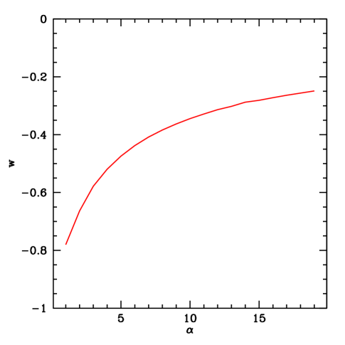
FIG. 10.: $w$ versus $\alpha$, with strongest allowed coupling $\xi$.

We have shown that certain classes of NMC quintessence models lead to a “natural” reduction in the primordial helium abundance. Although we have concentrated on the negative power law potentials, our results generalize easily to other potentials. In particular, one of the major problems with exponential potentials is that they lead to an overproduction of helium [24]. This problem could be ameliorated in the way we have suggested. Of course, the tracker solution for such models generically predicts $w=0$ at present [24] and thus these models have problems matching other observations. We also expect that these results would be changed if we used a different coupling between $Q$ and $R$ than that in Eq. (4). Thus, it might be possible to obtain even larger values for $\Delta Y$ in such models.

- [1] Electronic address: xuelei@pacific.mps.ohio-state.edu.
- [2] Electronic address: scherrer@pacific.mps.ohio-state.edu.
- [3] Electronic address: steigman@pacific.mps.ohio-state.edu.
- [4] A. G. Riess et al., Astron. J. 116, 1109 (1998); P. M. Garnavich et al., Astrophys. J. 509, 74 (1998); S. Perlmutter et al., Astrophys. J. 517, 565 (1999).
- [5] S. D. M. White, J. F. Navarro, A. E. Evrard and C. S. Frenk, Nature 366, 429 (1993).
- [6] P. de Bernardis et al., Nature 404, 955 (2000); S. Hanany et al., Astrophys. J. Lett. 545, 5 (2000); A. H. Jaffe, astro-ph/0007333.
- [7] S. Weinberg, Rev. Mod. Phys. 61, 1 (1989).
- [8] I. Zlatev, L. Wang and P. J. Steinhardt, Phys. Rev. Lett.82, 896 (1999).
- [9] P. J. Steinhardt, L. Wang, and I. Zlatev, Phys. Rev. D59, 123504 (1999).
- [10] A. R. Liddle and R.J. Scherrer, Phys. Rev. D59, 023509 (1999).
- [11] J.-P. Uzan, Phys. Rev. D59, 123510 (1999).
- [12] L. Amendola, Phys. Rev. D60, 043501 (1999).
- [13] T. Chiba, Phys. Rev. D60, 083508 (1999).
- [14] F. Perrotta, C. Baccigalupi, S. Matarrese, Phys. Rev. D61, 023507 (2000).
- [15] D.J. Holden and D. Wands, Phys. Rev. D61, 043506 (2000).
- [16] C. Baccigalupi, S. Matarrese, F. Perrotta, Phys. Rev. D62, 123510 (2000).
- [17] J.M. O’Meara, D. Tytler, D. Kirkman, N. Suzuki, J.X. Prochaska, A.M. Wolfe, Astrophys. J., submitted, astro-ph/0011179.
- [18] K. A. Olive and G. Steigman, Astrophys. J. Supp. 97, 49 (1995).
- [19] Y. I. Izotov and T. X. Thuan, Astrophys. J. 500, 188 (1998).
- [20] For a review, see e.g. P. Langacker, Nucl. Phys. B(Proc. Suppl.)77, 241(1999).
- [21] B. Ratra and P. J. E. Peebles, Phys. Rev. D 37, 3406 (1988)
- [22] L. Wang, R.R. Caldwell, J.P. Ostriker, and P.J. Steinhardt, Astrophys. J. 530, 17 (2000).
- [23] D. E. Groom et al. (PDG), Euro. Phys. J. C15, 1 (2000).
- [24] P. G. Ferreira and M. Joyce, Phys. Rev. Lett. 79, 4740 (1997), E. J. Copeland, A. Liddle and D. Wands, Phys. Rev. D 57, 4686 (1998).