Adaptive binning of X-ray galaxy cluster images

Abstract

We present a simple method for adaptively binning the pixels in an image. The algorithm groups pixels into bins of size such that the fractional error on the photon count in a bin is less than or equal to a threshold value, and the size of the bin is as small as possible. The process is particularly useful for generating surface brightness and colour maps, with clearly defined error maps, from images with a large dynamic range of counts, for example X-ray images of galaxy clusters. We demonstrate the method in application to data from Chandra ACIS-S and ACIS-I observations of the Perseus cluster of galaxies. We use the algorithm to create intensity maps, and colour images which show the relative X-ray intensities in different bands. The colour maps can later be converted, through spectral models, into maps of physical parameters, such as temperature, column density, etc. The adaptive binning algorithm is applicable to a wide range of data, from observations or numerical simulations, and is not limited to two-dimensional data.

1 Introduction

A problem often encountered with the processing of images, especially those from X-ray telescopes, is that there is a large dynamic range present in intensity. In order to examine the structure of emission in regions of an image where there are few photons, it is necessary to bin the data using bins of large angular size. An alternative is to smooth the data with a Gaussian kernel of large angular size. Conversely, to examine structure in areas of high emission, a small bin-size or kernel is sufficient. If one wishes to examine regions with a wide variation in count-rate, then some procedure which has a variable bin or kernel is required to create statistically optimal maps.

Another related problem, which motivated the present work, is the creation of optimal colour maps. The ratio of photon counts in a low intensity region will have a large associated statistical error, so the counts need to be averaged over a large region to form the ratio. The algorithm needs to account for the statistical accuracy in the separate bands, not just the total image.

One technique which allows structure on a wide range of scales to be revealed is adaptive kernel smoothing (Ebeling, White & Rangarajan 2000; Huang & Sarazin 1996). The asmooth algorithm of Ebeling et al. (2000) convolves an image with a Gaussian kernel. If the signal within the kernel, applied to part of an image, is of a chosen minimum significance above the local background, then the convolved signal is added to the output image. The kernel is increased in size until all the counts in the input image are added to the output image.

asmooth is very good at finding low surface brightness features, such as filaments. It also especially useful for producing images for display, and for identifying bright features against a background. It is not a universal smoothing tool, however, and care needs to be taken before using it in a particular situation. For instance, it is designed to identify positive features against a background, but not to identify ‘holes’ in emission. Due to the way it identifies significance against the local background, it may produce spurious features in areas where there is bright flat emission, for instance the cores of galaxy clusters, where Poisson noise may become significant. Used with care, asmooth is a useful routine in many situations.

The analysis method outlined in this paper, adaptive binning, was originally developed to produce temperature, column density and colour maps of the Perseus cluster in Fabian et al. (2000). We required a simple algorithm to compare the relative fluxes in different X-ray bands to a theoretical plasma emission model. In order to be able to spatially resolve the ratios, it is necessary to bin or smooth the data. Binning, rather than smoothing, is a better method for producing spatial estimates of counts for analysis, because it does not spread counts around an image beyond the boundaries of the bin.

In this paper we use data analysed from the 24 ks ACIS-S Chandra X-ray observation of the Perseus Cluster, Abell 426, from Fabian et al. (2000), to demonstrate the adaptive binning method. The Perseus Cluster is the brightest X-ray cluster in the sky, and contains a large cooling flow (Fabian et al. 1994) with a mass deposition rate of approximately $300\hbox{$\hbox{$\rm\thinspace M_{\odot}$}{\rm\thinspace yr}^{-1}\,$}$. Interesting substructure in the cluster due to its central radio source makes it an ideal object for our purpose. We will not attempt here to analyse the physics behind the observations, which is left to Fabian et al. (2000) and further work. We also study the method by applying it to simulated data.

The algorithm is presented in a logically consistent way, from intensity adaptive binning to colour adaptive binning. Colour binning, as mentioned above, was our original motivation, developed to analyse X-ray colour cluster images.

2 Intensity binning

Adaptive intensity binning is the simplest case of the algorithm. It attempts to adaptively bin a single image based on the number of photons in each region. The basic method is to bin pixels in two-dimensions by a factor of two, until the fractional Poisson error of the count in each bin becomes less than or equal to a threshold value. When the error is below this value, those pixels are not binned any further. The algorithm, in detail, is as follows.

1. Each pixel in the image is put into its own ‘bin’, the term we use for a collection of pixels. A pixel here means one of the individual picture elements which form the input image. Essentially the image is initially divided into imaginary $1\times 1$ pixel bins.

2. If there are $n_{i}$ pixels in bin $i$, the total count in the bin is $c_{i}$, and the background per pixel is $b$, the net count in the bin is simply defined by

   $$s_{i}\equiv c_{i}-n_{i}b.$$ (1)

3. The fractional error on the net count in the bin is

   $$\frac{{\sigma}_{\left(s_{i}\right)}}{s_{i}}=\frac{\sqrt{c_{i}+n_{i}b}}{c_{i}-n_{i}b}.$$ (2)

   This is also the error on the average count in each pixel.

4. If the fractional error is less than or equal to a threshold value, then the pixels in the output image which correspond to the pixels in the input bin are set to the average mean count, $s_{i}/n$. The fractional error of the net count in the bin is also stored in the pixels in an ‘error image’. Additionally the bin is marked as having been processed.

5. Each bin is merged into its neighbouring three bins, to make new bins containing $2\times 2$ of the previous bins. The four bins with the lowest $x$ and $y$ coordinates (lowest declination and highest right-ascension) are merged, as is each consecutive set of four bins. Any bins which have already been processed are ignored in the merging. It is useful to remember we are considering a bin as a list of pixels. Pixels which have already been set in the output image are ignored in future iterations.

6. The process is repeated from 1 until there is only a single bin remaining.

7. A ‘bin-map’ is also produced by the algorithm, giving an identification number for each processed bin in terms of the pixels which it contains. Using the bin-map, any image of that size can be binned using the same bins.

2.1 Demonstration

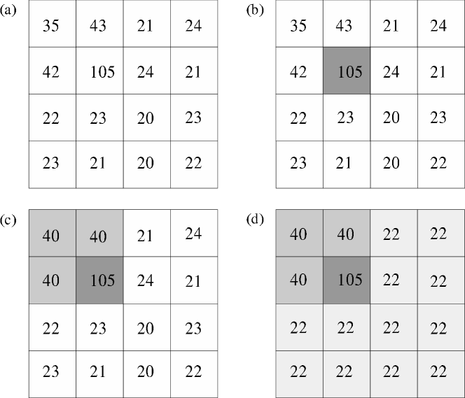
A simple demonstration of the algorithm operating on a $4\times 4$ pixel image is shown in Fig. 1. We demonstrate the process using a threshold fractional error of 0.1 and no background counts. (a) shows the image before binning. We first look for individual pixels (bins of $1\times 1$ pixels) with a Gaussian fractional error in the count less than or equal to the threshold. Only one pixel does; it is shown ‘painted’ in (b). We then bin the remaining pixels by a factor or 2. We examine the binned pixels to see whether any have errors less than the threshold. The three pixels in the top-left corner do, so they are averaged together and painted in (c). We then bin again with a $4\times 4$ pixel bin. The remaining pixels have an error less than the threshold, so they are averaged and painted in (d), the final output image. Had the error on the final bin been larger than the threshold, it would have been binned anyway.

Figure 1: Example demonstrating the intensity adaptive binning process. The bottom-left pixel is the origin, $(0,0)$. See the text for details.

2.2 Real example

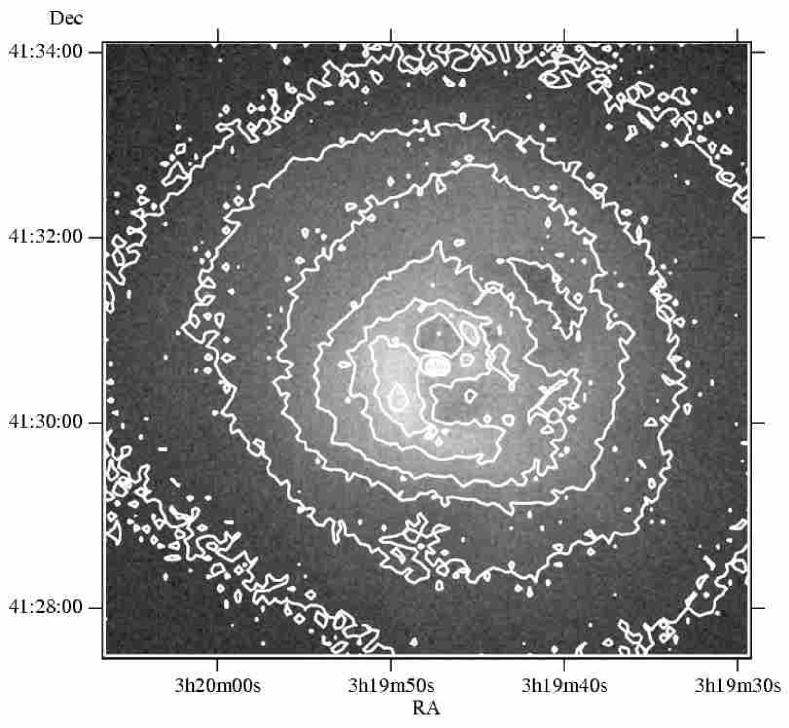
We show in Fig. 2 a ‘raw’ image of the Perseus cluster in the 0.5–7 keV band from the Chandra observation, binned with 2 arcsecond pixels. The image has been exposure-corrected. It also has been corrected for the readout node lines of the ACIS-S detector (this smears out the point source at the centre). Contours were placed on the image showing 8 levels spaced equally in square-root space between 20 and 300 counts.

The Perseus Cluster is very bright, so we see much structure in the data without doing more than simple binning. The contours shown have been smoothed, but even they break up at large radii due to the count rate being swamped by Poisson noise.

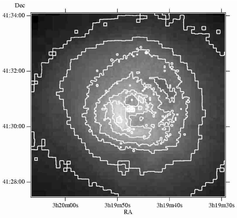
Fig. 3 shows the raw image of Perseus adaptively binned with a threshold fractional error of 0.06. The X-ray background was ignored since it was low, even near the image edges. The contours on the image near the centre match the contours in the raw data well, showing the algorithm works in this regime. At the sides, the bins are quite large and blocky, but otherwise there do not appear to be any edge-effects. There is still noise present in the image, but at a level much reduced from the raw data.

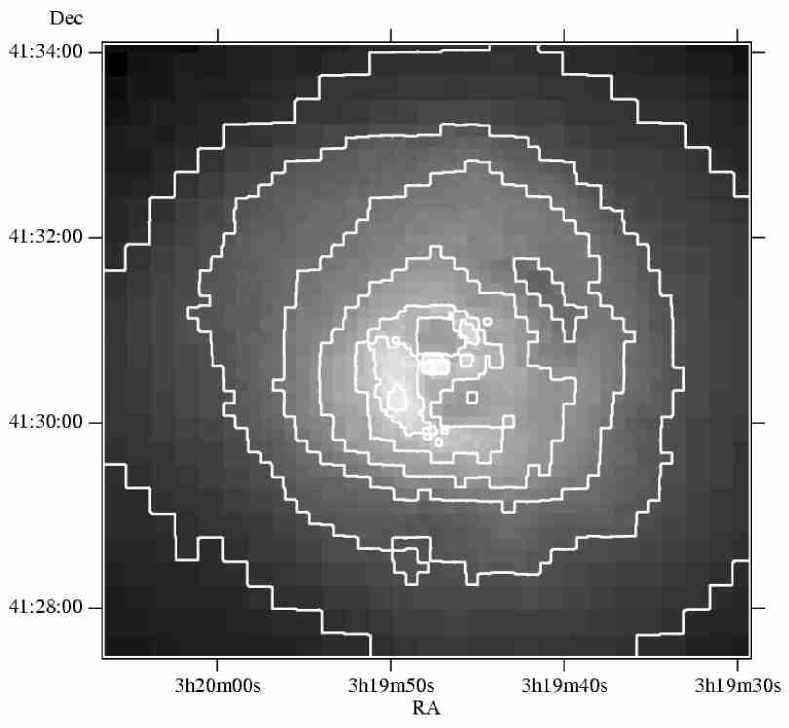
Fig. 4 shows the cluster again adaptively binned, but now with a threshold error of 0.04. Note how the bins are larger, but the level of noise is significantly less. A real feature has been lost from the image, however. A point source present in the upper left radio lobe has disappeared. Its counts were merged into rest of the emission from that region.

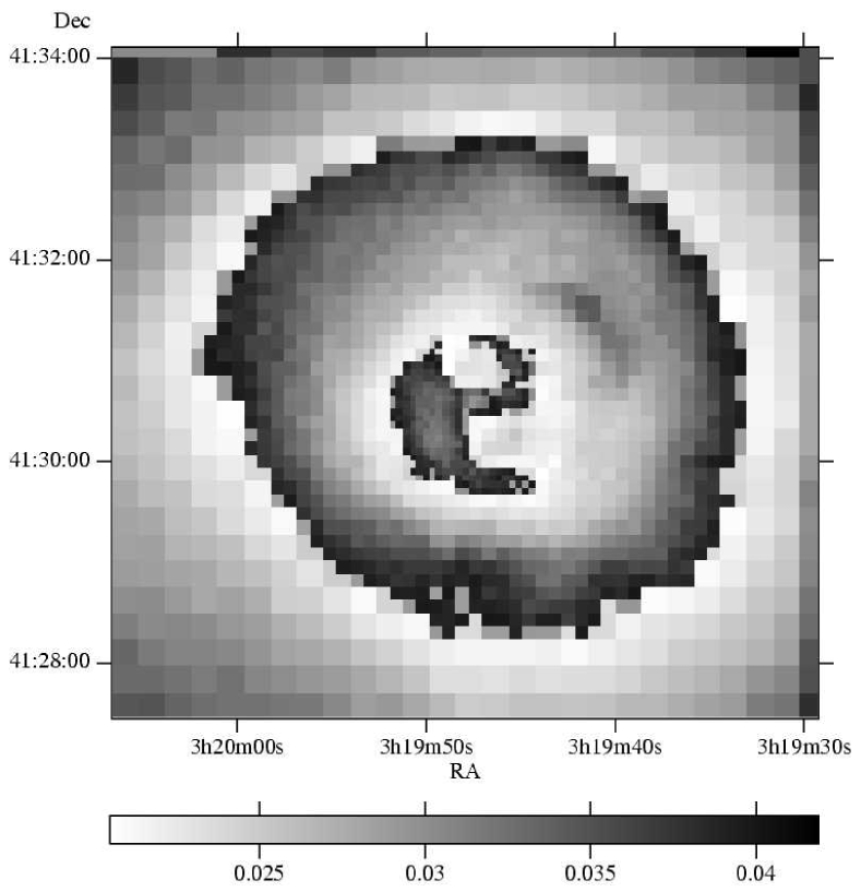
In Fig. 5 is shown the error map for the adaptively binned map above. In it are easily visible the changes in bin size as the count rate decreases towards the outside. As the count rate decreases, the error of the bins increases until it reaches the threshold, and then the bin-size doubles.

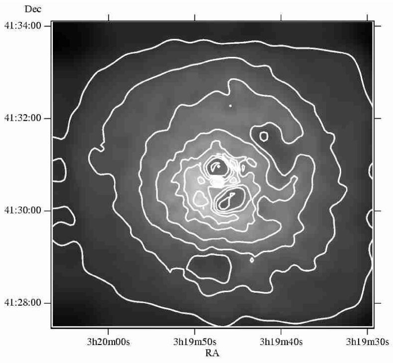
For comparison, Fig. 6 shows an adaptively smoothed (AS) image of the cluster calculated from the data in Fig. 2. It was smoothed with a minimum significance of 4–$\sigma$ using the asmooth algorithm of Ebeling et al. The contours are at the same levels as the raw image.

The AS image contains sharp positive features, such as the edges of the radio lobes. It does not perform as well in the determination of the number of counts in the negative features, such as the radio lobes themselves, where the number of counts per pixel is half that of the raw data. However, the algorithm is designed to find positive features, so using it to look at holes is a misapplication. Also apparent are some edge effects, where asmooth does not find enough counts to place a high significance on the generated features. The edge effects are avoidable by smoothing a larger area of sky than required, and cropping the image thereafter. One disadvantage of this is that asmooth running time increases quickly with image size.

Figure 2: Image of cluster binned with 2 arcsec pixels. The image has been corrected for exposure and readout node lines. 8 contours are spaced on a square-root scale, between 20 and 300 counts per pixel.

Figure 3: Adaptively binned image of the cluster. The pixel fractional error is set as 0.06. The contours are at the same levels as Fig. 2.

Figure 4: Adaptively binned image of the cluster. The pixel fractional error is set as 0.04. The contours are at the same levels as Fig. 2.

Figure 5: Fractional error map for adaptively binned image in Fig. 4.

Figure 6: Adaptively smoothed image of the cluster, with a minimum significance of 4–$\sigma$. The contours are at the same levels as Fig. 2. Note the edge effects in the contours.

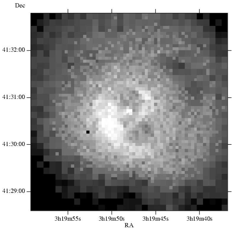
In Fig. 7 we show another adaptively binned image of the Perseus cluster. This, however, was created from data from an observation using the ACIS-I detector on Chandra, with an exposure of 18.6 ks. We present it because the number of counts per pixel is lower than the ACIS-S image, and so it is a good demonstration of the algorithm used on data with more noise.

Adaptive binning of the ACIS-I image brings out an interesting feature of the cluster; it clearly demonstrates that the southern rim of the northern radio lobe (hole) lies south of the nucleus. There is a linear diagonal structure present to the south of the nucleus, running from the north-west to the south-east. This structure is also present in the raw data, but is not clear on the ACIS-S image, despite the longer exposure, as the ACIS-S raw image contains a dark strip due to the node-line of the detector, where the effective exposure is short.

The dark bin to the south-east of the nucleus shows a ‘stranded bin’, an occasional problem with the algorithm, which we discuss later.

Figure 7: ACIS-I adaptively binned image of the Perseus cluster, using a fractional error of 0.15.

2.3 Notes on the algorithm

2.3.1 General

1. The algorithm allows bins of width $n$ to contain pixels with coordinates $(x,y)$ in the range $ni\leq x<n(i+1)$, $nj\leq y<n(j+1)$, where $i$ and $j$ are integers, and $i\geq 0$, $j\geq 0$. The coordinate origin is $(0,0)$. $x$ and $y$ increase in the directions of decreasing right-ascension and increasing declination, respectively.

2. If the unbinned image does not have sides which are an equal length of pixels, or are not a power of two, then the bins on one or both sides will be truncated. This can lead to bins with a small numbers of counts and a large error on the final pass.

3. As is the case with conventional binning, sources with small spatial extent may be split between two bins if they cross a bin boundary. This can be solved by allowing sub-bin positioning, described as follows. For each pass, bins are allowed to be placed at positions displaced by a multiple of some fraction of their length from their conventional positions. The errors are calculated for each possible bin, and the bins are sorted into order of ascending error, discarding those with an error larger than the threshold. The bins are painted in that order, ignoring those bins which had already been partially painted.

   The disadvantage of this technique is that the output image appears ‘dithered’. Bins are painted close to one another, but without enough space to put another bin between them. The result is a loose cluster of small bins inside a larger one. The original algorithm appears to produce better results and is less dependent on small variations of errors.

4. The bins are doubled in size between each pass, rather than slowly increased in size, as this ensures a whole number of smaller bins fit inside a larger bin. If this is not the case, then gaps are left between bins in the binning, leading to dithering.

5. Allowing rectangular bins is not useful. It is ambiguous in which direction a rectangle could lie, or be extended. Their use could introduce spurious linear structures into the output image.

6. The use of non-square bins is a possible technique. Any two dimensional object that tiles together could be used, but it is not clear what is the optimal shape. Square bins are a good choice for a number of reasons, including the fact that pixels are naturally square in most detectors; square bins act as scaled pixels. However, there is probably some room for additional work to find better shapes. An alternative idea is to use contour levels in an AS image to define ‘bins’, as demonstrated by Sanders, Fabian & Allen (2000).

2.3.2 Overlayed colour images

The adaptive-binning algorithm is useful for producing images demonstrating in real colour where the soft, medium and hard areas of emission are. First an intensity image can be binned to produce a bin-map. Then images in three energy bands can be binned themselves using the bin-map. A software package such as gimp can then be used to combine the three images as, for example, the red, green and blue layers in a single image. The contrast of the image can then be increased to highlight the areas of hard and soft emission.

The advantage of doing this rather than using raw data to make the image, is that the low-intensity regions are not dominated by noise. The technique was used to create the colour image of the Perseus cluster in Fabian et al. (2000).

2.3.3 Stranded pixels and contiguous regions

One ‘feature’ of the algorithm is that pixels may become ‘stranded’. If a bin has a reduced count relative to its neighbours, it may be left out on a pass and have no nearby pixels to be binned with on the next. It may be left until the final pass, and that area will be binned with the remaining pixels. Such pixels could be cosmetically removed by replacing them with their original value.

A modified version of the algorithm avoids stranded pixels. If a bin consists of more than one non-contiguous sets of pixels, then the bin is split into several contiguous regions, and each region treated by itself. A stranded set of pixels will remain until the end, where it will be binned by itself, as it is isolated. Here, two pixels are said to be connected if one pixels is one of the neighbouring eight pixels of the other pixel.

This modification has a couple of disadvantages. Firstly, finding contiguous sets of pixels is fairly slow. Also, parts of the image which would be connected were the image larger, are treated by themselves, and therefore have a larger statistical error on their count. With these problems in mind, it is probably a useful modification for many applications of the algorithm. For simplicity, we will use the unmodified version of the algorithm in the following sections.

2.4 Simulated cluster

In order to properly test the properties of the algorithm, we attempted to simulate a simple image of a cluster. We used a $\beta$-model to simulate the cluster with the following form (Sarazin 1988):

$$S_{b}(r)=S_{0}\left[1+\left(\frac{r}{r_{c}}\right)^{2}\right]^{0.5-3\beta},$$ (3)

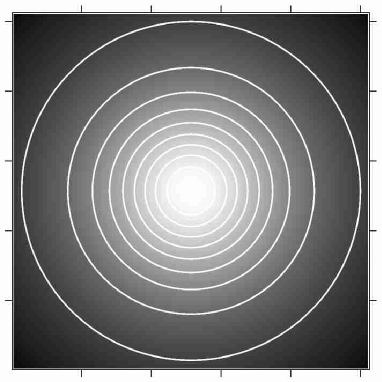
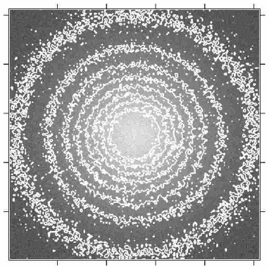
where $S_{b}$ is the surface brightness at a radius $r$, $r_{c}$ is a critical radius and $\beta$ is a parameter. We created an image of $512\times 512$ pixels, where $r_{c}$ was 128 pixels, $S_{0}$ was 100 counts/pixel, and $\beta$ was 0.67. The meaning of the word count, as used here for surface brightness, is the expectation value of an observation, and is allowed fractional values. The cluster was positioned in the centre of the image. It is shown in Fig. 8(a). The contours show constant surface brightness from 10-90 counts in linear 10 count intervals.

To simulate how such a cluster would appear, if observed, we took the surface brightness at a particular pixel, and randomly generated a value from a Poisson distribution with that surface brightness as the expectation value, to which we added a background with an expectation value of 20 counts/pixel. The Poisson image is shown in Fig. 8(b), with contours between 30 and 100 with the 10 count intervals. The contours are further out because of the background. The data was smoothed in contouring, as it was too noisy otherwise.

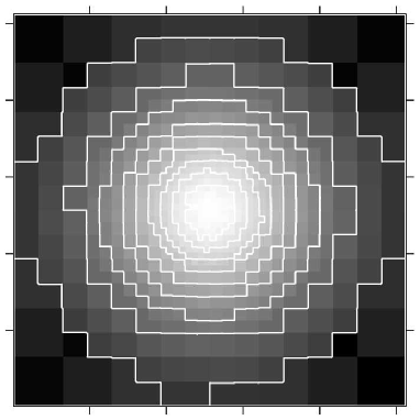
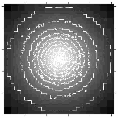
We processed the Poisson simulated data with our adaptive binning algorithm to produce Fig. 8(c). Here a fractional error threshold of 0.02 was used. Fig. 8(d) shows the output of the method using a threshold of 0.04, i.e. twice as large a threshold as (c). The contours are at the same levels as the original surface brightness image.

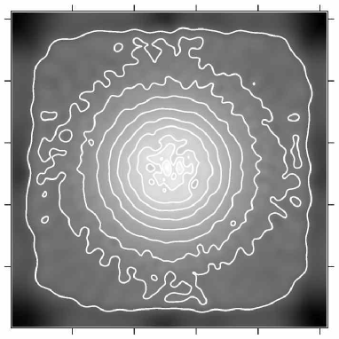
For comparison, we show the output from the asmooth program using a minimum feature significance of 4-$\sigma$ in Fig. 8(e). asmooth, by default calculates the local background and does not take a global value. To create this image we smoothed the simulated data and subtracted the background manually. The count per pixel becomes negative in the outer regions, as asmooth does not know about the global background, which also means features shown may have a lower significance than 4-$\sigma$.

(a)	(b)
(c)	(d)
(e)

Figure 8: Simulated cluster images. (a) Model surface brightness, contours range 10-90. (b) Simulated observation of cluster, contours range 30-100. (c) Adaptively binned image of cluster with error threshold of 0.02, contours range 10-90. (d) Adaptively binned image of cluster with error threshold of 0.06, contours range 10-100. (e) Adaptively smoothed image of cluster, $\sigma_{\mathrm{min}}=4$, contours range 10-100.

2.4.1 Spatial distributions of differences

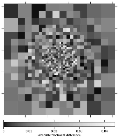
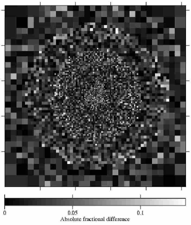
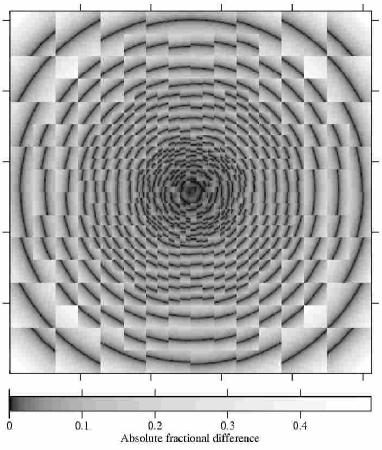
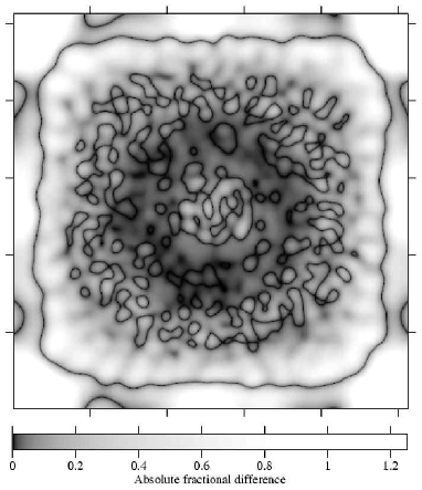
We constructed in Fig. 9 images displaying the absolute fractional differences between the reconstructed and model surface brightness images. Spatial correlations in errors should be visible on the images.

Fig. 9(a) shows the absolute differences between an adaptively binned image with 0.02 fractional errors (Fig. 8(c)), and the original surface brightness image binned with the same bins. (b) shows the same except using bins constructed for 0.06 fractional errors (Fig. 8(d)). There do not appear to be any correlations between the two images, in terms of where the differences are large and small. The differences appear noise-like and random. Note, however, that if the adaptively binned image were binned with inappropriate bins, then this would not show in (a) and (b) due to the surface brightness image being binned with the same bins.

Fig. 9(c) is an image showing the absolute differences between adaptively binned image with 0.02 fractional errors and the unbinned surface brightness image. Due to the count rate varying across the bin, only the centres have a low absolute fractional difference. This would be the same for any binning process.

Fig. 9(d) shows the differences between the AS image in 8(e) and the surface brightness image for comparison. Visible are the edge effects of the algorithm. Also present are some peaks at the cluster core. These are due to the local background estimation of the algorithm measuring significant detections against the flat core of the cluster centre.

(a)	(b)
(c)	(d)

Figure 9: Absolution fractional differences between the reconstructed images and original surface brightness image. (a) Adaptively binned image, error 0.02, and binned surface brightness image. (b) Adaptively binned image, error 0.06, and binned surface brightness image. (c) Adaptively binned image, error 0.02 and unbinned surface brightness image. (d) Adaptively smoothed image, $\sigma_{\mathrm{min}}=4$ and unbinned surface brightness image.

2.4.2 Histograms of differences

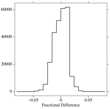
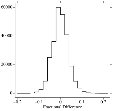
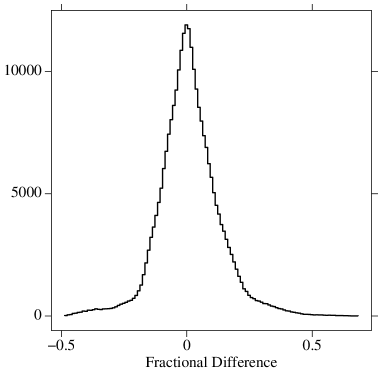
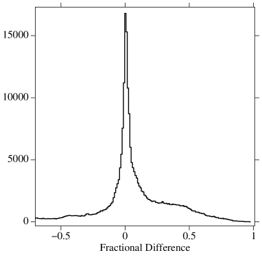
A more useful and quantitative analysis of the performance of the adaptive binning algorithm can be made by plotting the fractional differences (the absolute value of which is in the above images) as histograms, shown in Fig. 10. (a) displays the difference between the 0.02 error adaptively binned image and the surface brightness image binned using the same bins for each pixel. (b) is the same as (a), except using 0.06 error binned images. (c) shows a histogram of the differences between the 0.02 error adaptively binned image and the unbinned surface brightness image. The difference between an image produced by asmooth (Fig. 8(d)) and the surface brightness image is shown in (d) for comparison.

Fig. 10(a) and (b) approximate Gaussian distributions. The widths of the distributions are close to the threshold fractional error values used by the algorithm, 0.02 and 0.06. (c) shows a wider distribution, which is obtained due to the count varying across the bin in the surface brightness image, but not in the adaptively binned image. The results in (a) and (b) give confidence in the effectiveness of the algorithm, as the distributions are symmetric and Gaussian.

The histogram for the AS image in (d) has a very narrow peak, but there are long tails, mainly due to the edge-effects. Excluding the outer region almost removes the tail.

We also analysed the differences between the input surface brightness image and the adaptively binned image using the $\chi^{2}$ statistic. If there are $S_{i}$ total counts in the surface brightness image in bin $i$, and $s_{i}$ in the adaptively binned image, and $n_{i}$ pixels in the bin, then the statistic is

$$\chi^{2}_{i}=\frac{(S_{i}-s_{i})^{2}}{S_{i}+n_{i}b}.$$ (4)

We plotted the distribution of $\chi^{2}$ for the bins in the adaptively binned image. It showed reasonable agreement with the distribution predicted for one degree of freedom.

(a)	(b)
(c)	(d)

Figure 10: The distribution of fractional differences between pixels in binned images. (a) is between an adaptively binned (0.02 fractional error) image and the original surface brightness image binned with the same bins. (b) is the same as (a) except using 0.06 fractional error image. (c) is between an adaptively binned image (0.02 fractional error) and the original surface brightness image. (d) is between a $\sigma_{\mathrm{min}}=4$ AS image and the original surface brightness image.

3 Colour binning

A simple way to investigate the inner structure of a cluster is to create X-ray images in different energy bands. The images can then be divided to show the areas of hard and soft X-ray emission, known as a colour image. Additionally plasma codes, such as the mekal thermal model, can be fitted to the relative counts, enabling one to map temperature, metallicity and absorption.

One faces a similar problem to the simple intensity binning problem. How can ratios of counts be formed so that the error on the result is accurate enough? A binning algorithm must be able to use the same size bins on the images to be divided, plus it must adapt its bin size to the counts in each of the bands, rather than just one.

The colour adaptive binning algorithm is similar to the intensity algorithm, except it uses an input image for each band, to produce an output image for each band. Each input image is binned using the same bins. The bins are defined by the error on a ‘combined colour’, which folds the ratios of all the bands, not the error on the intensity. If $s^{i}_{k}$ is the background-subtracted count in band $i$ for bin $k$, the combined colour is defined as

$$C_{k}=\left[\left(s^{1}_{k}/s^{2}_{k}\right)/s^{3}_{k}\right]/\cdots.$$ (5)

The fractional error on the combined colour, if there are $N$ bands, is

$$\frac{\sigma_{\left(C_{k}\right)}}{C_{k}}=\left[\sum_{i=1}^{N}{\frac{c^{i}_{k}+n_{k}b^{i}}{\left(c^{i}_{k}-n_{k}b^{i}\right)^{2}}}\right]^{1/2}.$$ (6)

This error is a useful quantity because it takes into account the count in each band in a symmetric way. To make an actual colour map, two binned output images are divided.

An alternative approach is to adaptively bin a total intensity image. The resultant bin-map can then be applied individually to each of the X-ray bands. Ratios can be formed by dividing the output images. This approach has its advantages when several bands are being used. If a sharp feature is only present in one band, then the source will be binned with a large bin using the combined-colour method, due to the large statistical uncertainty on the colour. However, binning using the total intensity leads to colours with larger range of errors than the combined-colour approach.

3.1 Real example

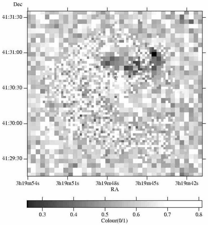
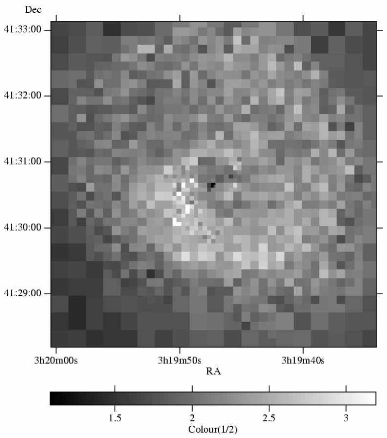
The combined colour adaptive binning method has been applied to the Perseus data shown earlier. Three images of the cluster were created in different bands, labelled from 0–2, in the energy ranges 0.5–1, 1–2 and 2–7 keV.

The colour adaptive binning algorithm above was applied to the data using a fractional errors on the combined colour, $\left(s^{0}/s^{1}\right)/s^{2}$, of 0.12 and 0.2. Again the background counts in each image were small enough to be neglected.

Fig. 11 shows the $s^{0}/s^{1}$ colour image produced with a fractional error of 0.2, which is sensitive to X-ray absorption; darker shades indicate more absorption. The absorption shadow of an infalling dwarf galaxy, discussed by Fabian et al. (2000), is clearly seen close to the centre of the image. The rest of the image has approximately uniform colour, indicating there are no further strong absorption features.

Fig. 12 shows the $s^{1}/s^{2}$ colour image produced with a fractional error of 0.12, which is sensitive to temperature; lighter shades indicate lower temperature. From this simple analysis, there appears to be a temperature gradient in the cluster, with cooler temperatures towards the centre and the brighter regions. This agrees with cooling flow models. The analysis emphasises a spiral structure, which is present right down to the cluster centre (compare with Fig. 7).

Using the combined colour method to generate the bins, the fractional errors on the bins for the individual colours, both range from 0.05 to 0.1 using a fractional error of 0.12. We have shown the colours with different fractional errors due to the relative strengths of features in the colours.

Figure 11: Colour map showing the ratio of counts in band 0 (0.5–1 keV) to band 1 (1–2 keV) for the Perseus cluster, adaptively binned with a fractional error of 0.2. This colour map highlights regions of high photoelectric absorption.

Figure 12: Colour map showing the ratio of counts in band 1 (1–2 keV) to band 2 (2–7 keV) for the Perseus cluster, adaptively binned with a fractional error of 0.12. This colour map highlights regions of low temperature.

3.2 Spectral fitting

As mentioned above, one can fit the relative counts in different X-ray bands against the relative counts predicted by a plasma code, to estimate physical properties, such as temperature and metallicity. To fit many parameters, several bands are required. It is useful to choose bands with approximately the same number of counts, the choice of which can be derived from the spectrum.

For a more detailed analysis, full spectral fitting is necessary. We have investigated taking an intensity-binned image of the object, automatically extracting spectra for each of the bins, automating xspec to fit each spectrum, and then plotting the fitted parameters spatially. As a side issue, the data must be binned so that there are enough counts per pixel to assume Gaussian errors. Also, spatial variations of the response matrix of the detector and telescope may need to be considered.

4 Availability

An implementation of the adaptive binning algorithm is available written in the C++ programming language. See the URL http://www-xray.ast.cam.ac.uk/~jss/adbin/ for instructions for download.

5 Summary

We have presented an algorithm to adaptively bin data. We have demonstrated its use on X-ray intensity and colour images of the Perseus cluster. We also applied the algorithm to simulated data. The method has also been used to create multi-layer colour images, where the colours represent the intensity in different bands. The fractional error threshold can be varied depending on how much statistical noise is acceptable in the analysed image.

The method is not limited to binning on intensity or colour. Any sort of data may be binned, providing there is a method to compute the statistical fractional error, or weighting, of a group of pixels. The algorithm may be useful in presenting the output from numerical simulations.

The method is also not limited to two-dimensional data. We have used it already on one-dimensional cuts through images. It may also be simply extended to work on $N$-dimensional data sets.

References

- [1] Huang Z. & Sarazin C., 1996, ApJ, 461, 622
- [2] Ebeling H., White D.A., Rangarajan F.V.N., MNRAS, 2000, in press
- [3] Fabian A.C., 1994, A&AR, 32, 277
- [4] Fabian A.C., Sanders J.S., Ettori S., Taylor G.B., Allen S.W., Crawford C.S., Iwasawa K., Johnstone R.M., Ogle P.M., 2000, MNRAS, 318, L65
- [5] Sanders J.S., Fabian A.C., Allen S.W., 2000, MNRAS, 318, 733
- [6] Sarazin C.L., 1988, X-ray emissions from clusters of galaxies. Cambridge