Probing Galaxy Formation with High Energy Gamma-Rays

Abstract

We discuss how measurements of the absorption of $\gamma$-rays from GeV to TeV energies via pair production on the extragalactic background light (EBL) can probe important issues in galaxy formation. We use semi-analytic models (SAMs) of galaxy formation, set within the hierarchical structure formation scenario, to obtain predictions of the EBL from 0.1 to 1000$\mu$m. SAMs incorporate simplified physical treatments of the key processes of galaxy formation — including gravitational collapse and merging of dark matter halos, gas cooling and dissipation, star formation, supernova feedback and metal production — and have been shown to reproduce key observations at low and high redshift. Here we also introduce improved modelling of the spectral energy distributions in the mid-to-far-IR arising from emission by dust grains. Assuming a flat $\Lambda$CDM cosmology with $\Omega_{m}=0.3$ and Hubble parameter $h=0.65$, we investigate the consequences of variations in input assumptions such as the stellar initial mass function (IMF) and the efficiency of converting cold gas into stars. We conclude that observational studies of the absorption of $\gamma$-rays with energies from $\sim$10 Gev to $\sim$10 TeV will help to determine the EBL, and also help to explain its origin by constraining some of the most uncertain features of galaxy formation theory, including the IMF, the history of star formation, and the reprocessing of light by dust.

I Introduction

The extragalactic background light (EBL) represents all the light that has been emitted by galaxies over the entire history of the universe. The EBL that we observe today is an admixture of light from different epochs, its spectral energy distribution (SED) distorted by the redshifting of photons as they travel to us from sources at different distances. It is therefore a constraint on both the intrinsic SEDs of the sources and their distribution in redshift. At present, there is more than a factor of two uncertainty in the amplitude of the EBL in the UV, optical, and near-infrared puget . The EBL in the mid-IR is even more uncertain. The far-IR background measured at $\lower 2.15277pt\hbox{$\;\buildrel>\over{\sim}\;$}100\mu$m puget96 ; guider97 ; hauser ; fixsen represents at least half of the total energy in the EBL, yet the sources that produced it remain uncertain.

High energy $\gamma$-ray astronomy promises to help resolve these uncertainties by providing independent constraints on the EBL, in the mid-IR with $E_{\gamma}$ in the $\sim 10$ TeV energy range, and in the 0.1-3 $\mu$m range with $E_{\gamma}\sim 100$ GeV via the new low-threshold instruments that will soon be available. High energy $\gamma$-rays from sources at cosmological distances are absorbed via electron-positron pair production on the diffuse background of photons that comprises the EBL. Thus, $\gamma$-ray observations of objects with known redshift and intrinsic spectral shape will constrain the EBL in these crucial wavelength regimes by measuring the optical depth of the Universe to photons of various energies. This in turn will help to constrain some of the most fundamental uncertainties in physical models of galaxy formation.

In order to illustrate this, in this paper we use a “forward evolution” approach, which attempts to model the essential features of galaxy formation using simple recipes. These semi-analytic models are set within the modern Cold Dark Matter (CDM) paradigm of hierarchical structure formation, and trace the gravitational collapse and merging of dark matter halos, the cooling and shock heating of gas, star formation, supernovae feedback, metal production, the evolution of stellar populations and the absorption and re-emission of starlight by dust. This machinery has been used extensively to predict optical properties of low-redshift galaxies, with good results (e.g., kwg ; cole94 ; reviewed and extended in sp ; spf , hereafter SP and SPF). A semi-analytic approach was also used by Devriendt and Guiderdoni dev2 to make predictions of counts and backgrounds in the mid-to-far-IR, with more detailed modelling of dust extinction and emission, but less detailed modelling of merging and star formation. We have now combined the strengths of these two models, by integrating the stellar SEDs and dust modelling of dev1 ; dev2 into the galaxy formation code of the Santa Cruz group.

Some parts of the “standard paradigm” of galaxy formation represented by our SAMs are relatively solid. For example, once a cosmological model and power spectrum are specified, it is straightforward to compute the gravitational collapse of dark matter into bound halos using $N$-body techniques, and analytic formalisms such as those used in our modelling sk have been checked against these results slkd . Within the range of values for the cosmological parameters allowed by existing observational constraints (i.e., $\Omega_{\rm matter}\simeq 0.3-0.5$, $\Omega_{\rm matter}+\Omega_{\Lambda}\simeq 1$, $H_{0}\simeq 60-80$ km/s/Mpc; see e.g. primack2000 for a summary), these results do not change significantly. Similarly, modelling of gas cooling appears to be fairly robust and agrees well with hydrodynamic simulations pearce . However, other aspects, notably the efficiency of conversion of cold gas into stars, the effect of subsequent feedback due to supernovae winds or ionizing photons, the stellar initial mass function (IMF), and the effects of dust, remain highly uncertain, and some predictions are quite sensitive to their details.

For example, SPF showed that the star formation history of the Universe and the number density of high redshift $z\lower 2.15277pt\hbox{$\;\buildrel>\over{\sim}\;$}2$ “Lyman-break” galaxies (LBGs; e.g. steidel:99 ) may be quite different depending on whether star formation is primarily regulated by internal properties, such as gas surface density in a quiescent disk, or triggered by an external event such as an interaction. Because the largest samples of LBGs are primarily identified in the rest UV, model predictions are also quite sensitive to the high-stellar-mass slope of the IMF, and to dust extinction. At the other end of the spectrum is the sub-mm population detected by SCUBA, believed to be predominantly high redshift ($z\lower 2.15277pt\hbox{$\;\buildrel>\over{\sim}\;$}2$) luminous and ultraluminous infrared galaxies (LIRGs and ULIRGs) powered by star formation rates of hundreds to thousands of solar masses per year (e.g., sanders ). Theoretical predictions of the numbers and nature of these objects are highly sensitive to the same issues (the dominant mode of star formation, dust, the IMF), but provide a crucial counter-balance to the optical observations. However, the current mismatch between the sensitivity and spatial resolution of optical and sub-mm instrumentation has made it difficult to establish the connection between the two populations observationally.

The Milky Way, like most nearby galaxies, emits the majority of its light in optical and near-IR wavelengths; only about 30% of the bolometric luminosity locally is released in the far-infrared sn:91 . This was generally believed to be typical of most of the starlight at all redshifts until the discovery of the far-IR part of the EBL by the DIRBE and FIRAS instruments on the COBE satellite, at a level ten times higher than the no-evolution predictions based on the local luminosity function of IRAS galaxies, and representing twice as much energy as the optical background obtained from counts of resolved galaxies madaupoz . This result suggests that either the dust extinction properties of “normal” galaxies change dramatically with redshift, or a population of heavily extinguished galaxies (perhaps analogous to local LIRGs and ULIRGs) is much more common at high redshift than locally, or both. Some of these galaxies may have already been observed, at 15 $\mu$m by ISO elbaz99 , and at 850 $\mu$m by SCUBA blain .

Guiderdoni et al. ghbm ; dev2 showed that their simplified semi-analytic model could reproduce the multi-wavelength data only if they introduced a population of heavily extinguished galaxies with high star formation rates, and with strong evolution of number density with redshift. This population was introduced ad-hoc by ghbm ; dev2 , but as discussed by these authors, by silkdev (based on bss ), and also by SPF, the increasing importance of starbursts at high redshift, due to the increasing merger rate and higher gas fractions, is a natural mechanism to produce this population. The models of SPF contain a detailed treatment of mergers and the ensuing collisional starbursts, which has been calibrated against the merger rate in cosmological $N$-body simulations kolatt and the starburst efficiency in hydrodynamical simulations mh ; somerville . Moreover, they produced good agreement with observations of LBGs and Damped Lyman-$\alpha$ systems (SPF) as well as low redshift galaxies (SP). Therefore, it will be extremely interesting to see if these same models, when combined with the more sophisticated treatment of dust extinction and emission developed by Devriendt, Guiderdoni, and collaborators, will be able to simultaneously reproduce observations over the broad range of wavelengths and redshifts discussed above.

In the next section we briefly describe the ingredients of our models, and then present the results of the predicted EBL. The following section presents the implications for $\gamma$-ray attenuation, and the final one briefly discusses some alternative treatments and our own conclusions. The work summarized here is a brief, preliminary sample of the results which will soon be presented in a series of papers, now in preparation, on the EBL and its breakdown into various kinds of sources and on the implications for $\gamma$-ray astronomy.

II Semi-analytic modelling

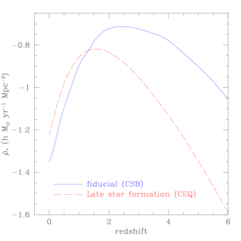
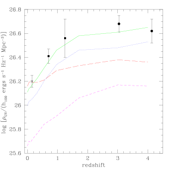
Figure 1: (a) The star formation rate density predicted by our models, for two different recipes of star formation. Both models produce about the same total mass density of stars by $z=0$ (i.e., the areas under the curves are equal when they are plotted linearly vs. time), but the collisional starburst model (CSB) peaks at higher redshift. (b) Comoving luminosity density at $2000\AA$ as a function of redshift. Data points represent the observed global luminosity density at rest $\sim 2000\AA$, obtained by integrating the observational best-fit Schechter luminosity functions over all luminosities ($\rho_{L}=\phi_{*}L_{*}\Gamma(2-\alpha)$). The $z=0.15$ point is from sullivan , the $z\sim 0.4$ and 1.2 points are from cowie , and the $z\sim 3$ and $z\sim 4$ points are from steidel:99 . The curves for our four models are labeled as in Figure 3. The model curves have been corrected for dust extinction using the approach described in the text.

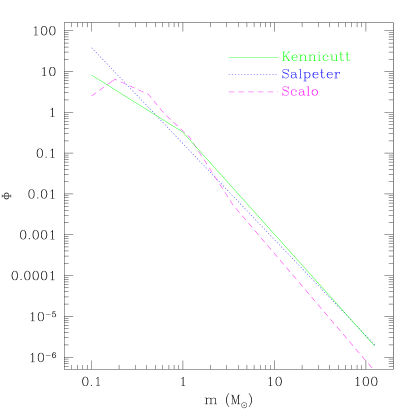
Figure 2: The three stellar Initial Mass Functions (IMFs) used here: Kennicutt kenIMF , Salpeter salpeterIMF , and Scalo scaloIMF .

In this section we briefly describe the ingredients of our models. Readers can refer to SP and SPF for more details, and to veritas for a brief introduction.

Using the method described in sk , we create Monte-Carlo realizations of the masses of progenitor halos and the redshifts at which they merge to form a larger halo. These “merger trees” (each branch in the tree represents a halo merging event) reflect the collapse and merging of dark matter halos within a specific cosmology. We truncate the trees at halos with a minimum circular velocity of 40 km/s, below which we assume that the gas is prevented from collapsing and cooling by photoionization. Each halo at the top level of the hierarchy is assumed to be filled with hot gas, which cools radiatively and collapses to form a gaseous disk. The cooling rate is calculated from the density, metallicity, and temperature of the gas. Cold gas is turned into stars using a simple recipe, depending on the mass of cold gas present and the dynamical time of the disk. Supernovae inject energy into the cold gas and may expell it from the disk and/or halo if this energy is larger than the escape velocity of the system. Chemical evolution is traced assuming a constant yield of metals per unit mass of new stars formed. Metals are initially deposited into the cold gas, and may later be redistributed by supernovae feedback, and mixed with the hot gas or the diffuse (extra-halo) IGM.

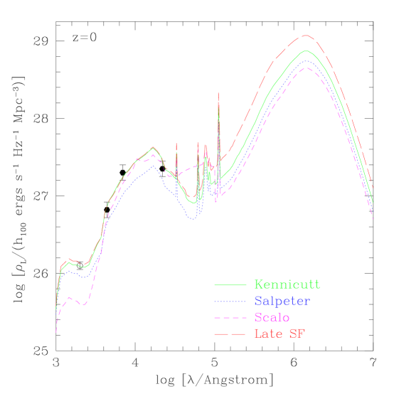
Figure 3: Comoving luminosity density at redshift $z=0$ as a function of wavelength. Data points represent the observed global luminosity density of the Universe, obtained by integrating the observational best-fit Schechter luminosity functions over all luminosities ($\rho_{L}=\phi_{*}L_{*}\Gamma(2-\alpha)$). The far-UV point (at $\lambda=2000\AA$) is from the luminosity function from FOCA observations sullivan , extrapolated from the mean redshift of the sample ($z=0.15$) to $z=0$ assuming that the luminosity density scales with redshift as $\rho_{L}\propto(1+z)^{1.7}$, as indicated by the observations of Cowie et al. cowie . The B-band point ($\lambda=4400\AA$) is from the luminosity function derived from the 2dF redshift survey folkes , the R-band point ($\lambda=6940\AA$) is from the Century Redshift Survey geller , and the K-band point ($\lambda=2.2\mu m$) is from gardnerK . The model curves are obtained by simply summing the spectra of all $z=0$ galaxies in our models with the appropriate Press-Schechter weighting.

When halos merge, the galaxies contained in each progenitor halo retain their seperate identities until they either spiral to the center of the halo due to dynamical friction and merge with the central galaxy, or until they experience a binding merger with another satellite galaxy orbiting within the same halo. All newly cooled gas is assumed to initally collapse to form a disk, and major (nearly equal mass) mergers result in the formation of a spheroid. New gas accretion and star formation may later form a new disk, resulting in a variety of bulge-to-disk ratios at late times.

For an assumed IMF, the stellar SED of each galaxy is then obtained using stellar population models. Here we use the multi-metallicity stellar SEDs of dev1 for the Salpeter and Kennicutt IMF cases, and the solar metallicity GISSEL models bc for the Scalo IMF. (We have found that using evolving metallicity rather than solar metallicity SEDs has a relatively small impact on the resulting EBL.) Dust extinction is modelled using an approach similar to that of dev2 . The optical depth of the disk is assumed to be proportional to the column density of metals. We then use a simple slab geometry where stars and gas are homogenously mixed, and assign a random inclination to each galaxy to compute the absorption. We use a metallicity dependent extinction curve, following ghbm ; dev2 .

All absorbed light is re-radiated at longer wavelength. In general, any galactic dust emission spectrum can by represented by a combination of three components: 1) hot dust (as in $H_{\rm II}$ regions), 2) warm dust (as in the diffuse $H_{\rm I}$), and 3) cold dust (as in molecular clouds). In the models of Devriendt et al. dev1 , these components are modelled as a mixture of polycyclic aromatic hydrocarbon molecules (PAH), very small grains, and big grains. Big grains may be either cold ($\sim$ 17 K), or heated by radiation from star-forming regions (as suggested by observations of typical local starburst galaxies like M82). A set of template spectra is then constructed for galaxies of varying IR luminosity, with admixtures of the various components selected in order to reproduce the observed relations between IR/sub-mm color and IR luminosity. A similar approach was used by dwek:98 , using a mixture of a typical Orion-like $H_{\rm II}$ spectrum and an $H_{\rm I}$ spectrum constructed to fit DIRBE observations of the diffuse ISM dwek:97 . Here, we use the more empirical emission templates of dwek:98 (kindly provided in electronic form by E. Dwek), but we obtain very similar results with the models of dev1 .

The recipes for star formation, feedback, chemical evolution, and dust optical depth contain free parameters, which we set for each model (see SP) by requiring an average fiducial “Milky Way” galaxy to have a K-band magnitude, cold gas mass, metallicity, and average B-band extinction as dictated by observations of nearby galaxies.

Figure 1a shows the global star formation rate density for the two star formation recipes that we consider here. The “fiducial” model is the collisional starburst (CSB) model favored by SPF, in which bursts of star formation may be triggered by galaxy collisions. The “Late star formation” model is the Constant Efficiency Quiescent (CEQ) model of SPF, in which cold gas is converted to stars only in a quiescent mode with constant efficiency. This produces a star formation history similar to the models of baugh , in which the peak in the star formation history occurs at a considerably later epoch ($z\sim 1.5$) than in the CSB model. Figure 3 shows the resulting luminosity density as a function of wavelength at $z=0$. For the CSB model, we consider three different choices of IMF: Scalo scaloIMF , Salpeter salpeterIMF , and Kennicutt kenIMF . These IMFs are graphed in Figure 2. For the CEQ model we show only the Kennicutt case. This is compared with the observed luminosity density from nearby galaxies, obtained by integrating the luminosity functions of galaxies resolved in recent redshift surveys at wavelengths ranging from 0.2 to 2.2 $\mu$m. The spikes in the model predictions at $\sim 5-12\mu$m are caused by the PAH features mentioned above. All four models, when normalized to the observed K-band Tully-Fisher relation, produce reasonable agreement with the observed luminosity density in the B and K bands. This is perhaps not surprising, yet it was not guaranteed. However, there is a noticable difference in the far-UV and the mid- to far-IR. The Scalo IMF produces too little UV light relative to optical and near-IR light, whereas the Kennicutt and Salpeter IMFs are in much better agreement with the data. These IMFs produce more high mass stars than the Scalo IMF, and thus more ultraviolet light to be absorbed and re-radiated by dust in the far IR. In Fig. 1b we show the redshift evolution of the far-UV ($2000\AA$) luminosity density, compared with observations. The Scalo model falls short at all redshifts, and the CEQ model, which agrees at $z=0$, falls short at higher redshifts. It is encouraging that our very simple model for dust extinction, which we normalized in the B-band at $z=0$, appears to yield the appropriate level of dust extinction in the UV at higher redshifts (SPF).

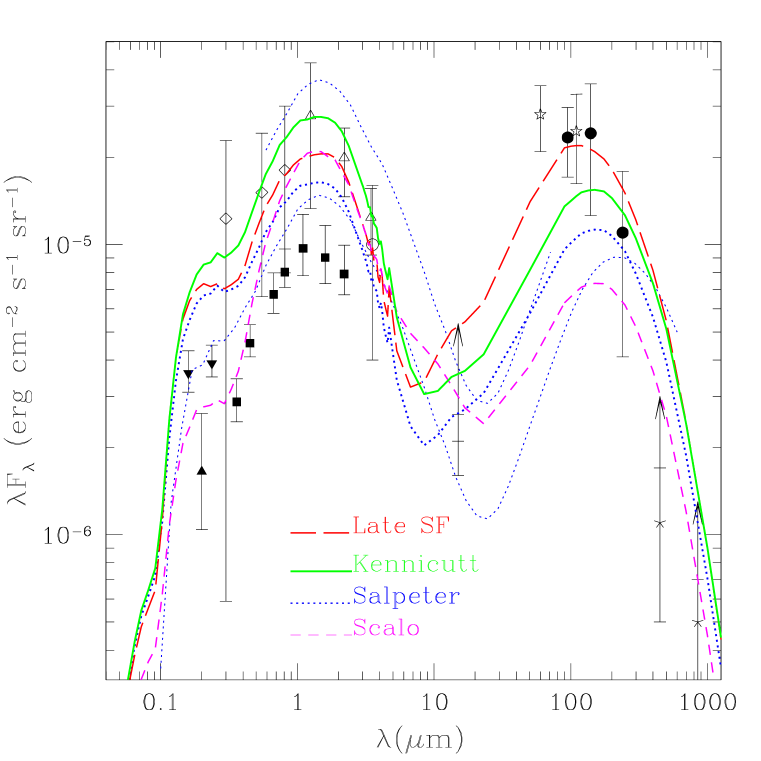
Figure 4: Extragalactic background light: models and data. The far-UV points are from STIS (inverted filled triangles) gardner and FOCA observations (filled triangle) foca . The lower optical points (filled squares) are lower limits from resolved sources madaupoz ; the upper ones (open diamonds) are from absolute photometry bernstein . The near-IR points are from DIRBE: (open circle) dwekarendt , (open triangles) wright . The point at 15 $\mu$m is from ISOCAM resolved sources elbaz99 , and is thus a lower limit. The far-IR points are from DIRBE (filled circles) hauser ; lagache , (stars) fds . The curves are our results from modelling the history of star formation in the $\Lambda$CDM cosmology using semi-analytic methods: a model with both quiescent star formation with constant efficienty and starbursts, with Kennicutt, Salpeter, and Scalo IMFs, and a model with only quiescent star formation with constant efficienty (Late SF). The lower light dotted curve is the $\Lambda$CDM EBL calculated using our previous methods veritas for the Salpeter IMF, and the upper one is the same curve to 80 $\mu$m multiplied by 2.5 for comparison with Mrk 501 data as analyzed by guy (see text). Note that $10^{-6}$ erg s^-1 cm^-2 sr^-1 = 1 nW m^-2 sr^-1.

III The Integrated Extragalactic Background Light

Figure 4 shows the EBL produced by our four models, obtained by integrating the light over redshift (out to $z=4$) with the appropriate K-corrections due to cosmological redshifting. We compare this with a compilation of observational limits and measurements of the EBL. It is apparent that there is at least as much energy in the far-IR part of the EBL as in the entire optical and near-IR bands. For example, Puget and collaborators puget estimated that the total energy in the EBL is between 60 and 93 nW m^-2 sr^-1, with between 20 and 41 nW m^-2 sr^-1 contributed by the optical and near-IR, and between 40 and 52 nW m^-2 sr^-1 coming from the far-IR. If the possible detection of the EBL at 60 $\mu$m by Finkbeiner et al. fds is correct, that would further increase the far-IR EBL; however, as Puget discussed in his talk at this conference, it is very difficult to determine the EBL at 60 $\mu$m since the zodiacal light is so much brighter at that wavelength.

In units of critical density $\rho_{c}$, $\Omega_{\rm EBL}=(4\pi/c)(I_{\rm EBL}/\rho_{c}c^{2})=2.5\times 10^{-8}I_{\rm EBL}h^{-2}$, where $I_{\rm EBL}$ is in units of nW m^-2 sr^-1. The total energy density in the EBL corresponding to the lower and upper estimates of puget is $\Omega_{\rm EBL}=(3.6-5.5)\times 10^{-6}(h/0.65)^{-2}$. Although the EBL includes energy radiated by active galactic nuclei (AGNs) as well as stars, it is unlikely that AGNs contributed more than a few percent of the total. The total energy radiated by AGNs is $E_{\rm EBL}^{\rm AGN}=\eta\rho_{\rm BH}c^{2}$, where the efficiency of conversion of mass to radiated energy in AGNs is $\eta\sim 0.05$. Correspondingly, $\Omega_{\rm EBL}^{\rm AGN}=\eta\Omega_{\rm BH}(1+z_{\rm BH})^{-1}\approx 4.5\times 10^{-8}h^{-1}(\eta/0.05)[3/(1+z_{\rm BH})]\lower 2.15277pt\hbox{$\;\buildrel<\over{\sim}\;$}0.02\Omega_{\rm EBL}$.  So for simplicity, in this paper we will neglect the contribution of AGNs to the EBL.

Several interesting features emerge from the comparison of our SAM models with the EBL data. In the UV to near-IR, the models are much closer to the direct measures of the EBL obtained by bernstein ; dwekarendt ; wright , although the Scalo IMF produces less light in the UV because it has fewer high-mass stars. Recall that the Kennicutt model agreed well with the observed luminosity density at $z=0$, and the observed redshift evolution of the luminosity density in the rest UV. This suggests that the extra factor of 2-3 in the direct measurements of the EBL must arise from a rapidly evolving population of objects which are too faint or too low in surface brightness to be detected in the samples used to obtain the counts (e.g., madaupoz ). We are in the process of attempting to determine whether the observational selection effects inherent in the measured counts are sufficient to explain this discrepancy for our modelled population. A second interesting point is that all the models satisfy the lower limits from counts in the mid-IR (15 $\mu$m; elbaz99 ) and the sub-mm (850 $\mu$m; blain ). Of our four new EBL curves, the Late SF model and the fiducial Kennicutt model are also consistent with the DIRBE/FIRAS measurements at 140 and 240 $\mu$m. The models differ significantly in the mid-IR, $\sim 10-60\mu$m, where the EBL can be probed by TeV $\gamma$-rays. The lower dotted curve, representing our previous attempt veritas to model the EBL, is well below the 15 $\mu$m lower limit as well as the DIRBE measurements at longer wavelengths. As we stated in veritas , we expected our EBL results to change as we improved our dust emission modelling. In addition to inclusion of the PAH features, the new dust emission model has more warm dust than the one used in veritas .

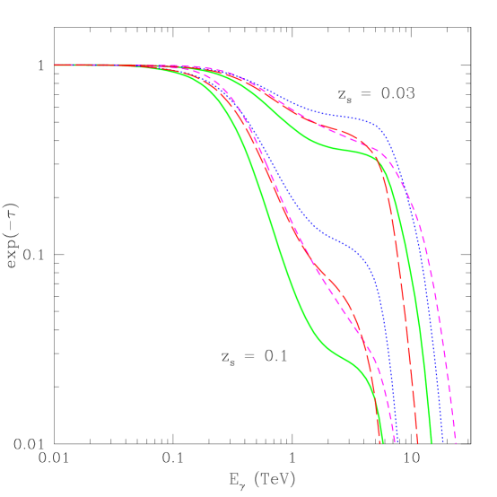
Figure 5: The attenuation factor, $\exp(-\tau)$ for $\gamma$-rays as a function of $\gamma$-ray energy for the four $\Lambda$CDM models considered in Fig. 4. The assumed redshift of the source, z_s, is indicated for each set of curves.

We now discuss constraints from the TeV $\gamma$-ray observations.

IV Attenuation of high-energy $\gamma$-rays

Figure 5 shows the $\gamma$-ray attenuation predicted by the four $\Lambda$CDM models considered here, for sources at redshifts $z_{s}=0.03$ and 0.10. All of the models predict rather little absorption at $E_{\gamma}\lower 2.15277pt\hbox{$\;\buildrel<\over{\sim}\;$}5$ TeV for sources at $z_{s}=0.03$, but fairly sharp cutoffs above 10 TeV, especially for the Late SF model. That model may be in conflict with the data from Mrk 501. The synchrotron self-Compton (SSC) model, in which $\sim$keV synchrotron X-radiation from a very energetic electron beam is Compton up-scattered by the same electrons to produce the observed $\sim$TeV $\gamma$-rays, appears to explain both the keV-TeV spectra and their time variation for the blazars Mrk 421 and 501, both at $z\approx 0.03$ (see, e.g., guy ; kraw99 and references therein). Using a simplified SSC model and keV X-ray data to predict the unattenuated TeV spectrum of Mrk 501, Guy et al. guy used CAT and HEGRA data to estimate the amount of $\gamma$-ray attenuation. They find that there is a rather good fit to the observed attenuation for the $\Lambda$CDM-Salpeter EBL from veritas when it is scaled upward by a factor of up to about 2.5 across the wavelength range 1-80 $\mu$m; this is the upper Salpeter curve on Fig. 4. The guy 1-$\sigma$ upper limit for 20-80 $\mu$m is a scaling factor of 3.4. Our new Salpeter curve appears to be rather consistent with this rescaling of our old Salpeter one, the Kennicutt curve may be a little high, but the Late SF curve appears to be definitely too high.

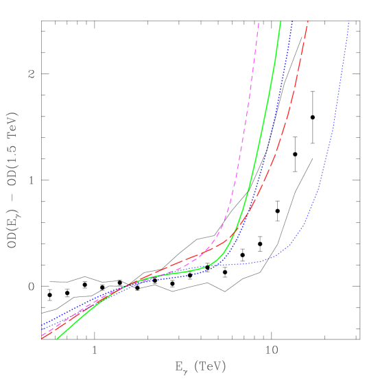
Figure 6: Increase of the optical depth (OD) for $\gamma$-rays due to intergalactic extinction, inferred from comparison of the observed Mrk 501 spectrum from HEGRA with that estimated using SSC models. The points correspond to Doppler factor $\delta_{j}=25$, magnetic field $B=0.037$ G; the upper and lower light solid curves correspond respectively to $(\delta_{j},B)=(100,0.012$ G) and (25,0.12 G), and the statistical error bars on the points also apply to these curves. The redshift of Mrk 501 z${}_{s}=0.034$ was used in calculating the optical depth for each model. This figure is based on Figure 10 of kraw99 .

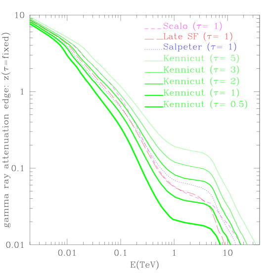
Figure 7: The $\gamma$-ray attenuation edge. The redshift where the optical depth reaches unity is shown as a function of $\gamma$-ray energy for each of the four $\Lambda$CDM models considered in Fig. 4. Also shown for the Kennicutt IMF is the redshift where the optical depth equals 0.5, 2, 3, and 5.

The compatibility of our new EBL calculations with the available data on TeV $\gamma$-ray attenuation is definitely worth further investigation. The results appear to be sensitive to the details of the models, raising the hope that they may be able to help answer important questions about star formation and dust reradiation, and also help to test the SSC modelling. For example, Figure 6 shows the optical depth as a function of $\gamma$-ray energy $E_{\gamma}$, compared with $\gamma$-ray attenuation results from Mrk 501 with detailed SSC models. This figure is like Fig. 10 of Krawczynski et al. kraw99 . While that figure showed OD($E_{\gamma}$) - OD(0.5 TeV), following Krawczynski’s advice we here plot OD($E_{\gamma}$) - OD(1.5 TeV), normalizing to the data at 1.5 TeV since the systematic error in the curvature of the spectrum strongly increases below 1.5 TeV, corresponding at 0.5 TeV to a flux uncertainty of 50%. (Krawczynski also kindly updated his model curves for this figure to take into account the 15% HEGRA energy uncertainty. We followed his advice to omit the highest-energy point, which has a statistical significance well below 2$\sigma$.) The conclusions from Fig. 6 appear to be consistent with those from our discussion of guy : the higher model curve seems compatible with our new Salpeter results, taking into account that the error bars on the data points also apply to the model curves; the Kennicutt model also appears to be consistent, except perhaps at the highest $E_{\gamma}$; and the Late SF model definitely predicts too much attenuation.

Figure 7 depicts the $\gamma$-ray “absorption edge,” the redshift of a source corresponding to an optical depth of unity, as a function of $\gamma$-ray energy. Travelling through the evolving extragalactic radiation field, $\gamma$-rays from sources at lower redshift suffer little attenution. The universe becomes increasingly transparent as $E_{\gamma}$ decreases, probing the background light at increasingly short wavelengths. (We are using the treatment of madau95 to account for absorption of ionizing radiation by the Lyman alpha forest.) The models all have the same qualitative features, but differ significantly quantitatively. The location of the absorption edge is affected both by the assumed IMF and by the history of star formation. There is more absorption at most redshifts with the Kennicutt IMF because with a higher fraction of high mass stars, it is more efficient at producing radiation for a given stellar mass; there is more absorption nearby in the Late SF model because the starlight in this model is less diluted by the expansion of the universe. It is possible that measuring the transparency of the universe to $\gamma$-rays at $\sim 0.1$ TeV with a number of sources at various redshifts can provide a strong probe of star formation, although there are uncertainties due to extinction by dust.

V Outlook

The semi-analytic modelling of the EBL described here follows the evolution of galaxy formation in time. Forward modelling is a more physical approach than backward modelling (luminosity evolution). Pure luminosity evolution (e.g., ms98 ; ms00 ; steckeriau ) assumes that the entire evolution of the luminosity of the universe arises from galaxies in the local universe just becoming brighter at higher redshift by some power of $(1+z)$ out to some maximum redshift. It effectively assumes that galaxies form at some high redshift and subsequently just evolve in luminosity in a simple way. This is at variance with hierarchical structure formation of the sort predicted by CDM-type models, which appears to be in better agreement with many sorts of observations.

An alternative approach to modelling the EBL has been followed by Pei and collaborators peifall95 ; fallcp ; pei99 , in which they find an overall fit to the global history of star formation subject to constraints from input data including the evolution of the amount of neutral hydrogen in damped Ly$\alpha$ systems (DLAS). Their first attempt peifall95 ; fallcp , which was used as the basis for EBL estimates by dwek:98 ; salamonstecker , was somewhat misled by the sharp drop in the DLAS hydrogen abundance from redshift $z\sim 3$ to $z\sim 2$ reported in lwt95 . With more complete data on DLAS (see, e.g., Fig. 14 of slw00 ) the $z=3$ neutral hydrogen abundance is lower and almost constant from $z=2$ to 4. The latest paper by Pei et al. pei99 takes a variety of recent data into account. Their approach is to follow the evolution of the total mass in stars, interstellar gas, and metals in a representative volume of the universe; they assume a Salpeter IMF. By contrast, the semi-analytic methods we use follow the evolution of many individual galaxies in the hierarchically merging halos of specific CDM models, here $\Lambda$CDM. Despite the differences in approach, and the fact that pei99 assumed $\Omega_{m}=1$ and Hubble parameter $h=0.5$, their results are broadly similar to those from the semi-analytic approach (see their §4.4; for our semi-analytic approach to modelling DLAS, see maller ). In particular, their EBL is similar to our old results veritas for the Salpeter IMF. Our EBL results presented here are higher in the near-IR and more consistent with the direct determinations dwekarendt ; wright ; they are also higher in the mid-IR, probably mainly because of the warm dust and PAH features in our dust emission model. It will be interesting to see whether further development of the global approach of Pei et al. and of the semi-analytic approach lead to convergent results.

As our calculations show, the EBL, especially at $\lower 2.15277pt\hbox{$\;\buildrel<\over{\sim}\;$}1$ $\mu$m and $\lower 2.15277pt\hbox{$\;\buildrel>\over{\sim}\;$}10$ $\mu$m, is significantly affected by the IMF and the absorption of starlight and its reradiation by dust, as well as by the underlying cosmology. The cosmological parameters are becoming increasingly well determined by other observations. As data become available on $\gamma$-ray emission and absorption from sources at various redshifts, especially from the new generation of Atmospheric Cherenkov Telescopes and the new $\gamma$-ray satellites AGILE and GLAST, these data and their theoretical interpretation will help to answer fundamental questions concerning how and in what environments all the stars in the universe formed.

References

- (1) Gispert R., Lagache G., and Puget, J.L., A&A 360, 1 (2000).
- (2) Puget J.L. et al., A&A 308, L5 (1996).
- (3) Guiderdoni B. et al., Nature 390, 257 (1997).
- (4) Hauser M.G. et al., ApJ 508, 25 (1998).
- (5) Fixsen D.J. et al., ApJ 508, 123 (1998).
- (6) Kauffmann G., White S.D.M., and Guiderdoni B., ApJ 264, 201 (1993).
- (7) Cole S. et al. 1994, MNRAS 271, 781 (1994).
- (8) Somerville R.S. and Primack J.R., MNRAS 310, 1087 (1999) (SP).
- (9) Somerville R.S., Primack J.R., and Faber S.M., MNRAS in press, astro-ph/0006364 (2000) (SPF).
- (10) Devriendt J.E.G. and Guiderdoni B., A&A in press, astro-ph/0010198 (2000).
- (11) Devriendt J.E.G., Guiderdoni B., and Sadat R., A&A 350, 381 (1999).
- (12) Somerville R.S. and Kolatt T., MNRAS 305, 1 (1999).
- (13) Somerville R.S., Lemson G., Kolatt T., and Dekel A., MNRAS 316, 479 (2000).
- (14) Primack J.R., in Sources and Detection of Dark Matter in the Universe (DM 2000), ed D.B. Cline, astro-ph/0007187 (2000).
- (15) Pearce F.R. et al., astro-ph/0010587 (2000).
- (16) Steidel C. et al., ApJ 519, 1 (1999).
- (17) Sanders D.B., Astrophys and Space Sci. 269/270, 381 (1999).
- (18) Soifer B.G. and Neugebauer G., AJ 101, 354 (1991).
- (19) Madau P. and Pozzetti L., MNRAS 312, L9 (2000).
- (20) Elbaz D. et al., in “The Universe as seen by ISO”, eds. P. Cox and M.F. Kessler, astro-ph/9902229 (1999).
- (21) Blain A., Smail I., Ivison R.J., and Kneib J.-P., MNRAS 302, 632 (1999).
- (22) Guiderdoni, B., Hivon, E., Bouchet, F.R., and Maffei, B., MNRAS, 295, 877 (1998).
- (23) Silk J. and Devriendt J., in “The Extragalactic Infrared Background and its Cosmological Implications”, eds M. Harwit and M.G. Hauser, astro-ph/0010460 (2000).
- (24) Balland C., Silk J., and Schaeffer R., ApJ 497, 541 (1998).
- (25) Kolatt T. et al., astro-ph/0010222 (2000).
- (26) Mihos C. and Hernquist L., ApJ 425, 13 (1994); 448, 41 (1995); 464, 641 (1996).
- (27) Somerville R.S. et al., to appear in the proceedings of the 15th IAP meeting, Paris, July 1999, Ed. F. Combes et al., astro-ph/9910346 (1999).
- (28) Sullivan M. et al., MNRAS 312, 442 (2000).
- (29) Cowie L.L., Songaila A., and Barger A.J., AJ 118, 603 (1999).
- (30) Primack J.R., Bullock J.S., Somerville R.S., and MacMinn D., Astroparticle Phys. 11, 93 (1999); Bullock J.S., Somerville R.S., MacMinn D., and Primack J.R., Astroparticle Phys. 11, 111 (1999).
- (31) Folkes S.R. et al., MNRAS 308, 459 (1999).
- (32) Geller M.J. et al., AJ 114, 2205 (1997).
- (33) Gardner J.P., Sharples R.M., Frenk C.S., and Carrasco B.E., ApJ 480, L99 (1997).
- (34) Bruzual G. and Charlot S., ApJ, 405, 538 (1993).
- (35) Dwek E. et al., ApJ 508, 106 (1998).
- (36) Dwek E. et al., ApJ 484, 779 (1997).
- (37) Baugh C.M., Cole S., Frenk C.S., and Lacey C.G., ApJ 498, 504 (1998).
- (38) Scalo J.M., Fund. Cosmic Phys. 11, 1 (1986).
- (39) Salpeter E.E., ApJ 121, 161 (1955).
- (40) Kennicutt R.E., ApJ 272, 54 (1983).
- (41) Sheth R. and Tormen G., MNRAS, 308, 119 (1999).
- (42) Gardner J.P., Brown T.B., Ferguson H.C., ApJ 542, L79 (2000).
- (43) Armand C., Milliard B., Deharveng J.-M., A&A 284, 12 (1994).
- (44) Bernstein R.A., Freedman W.L, and Madore B.F. in preparation (2000).
- (45) Dwek E. and Arendt R.G., ApJ 508, L9 (1998).
- (46) Gorjian V., Wright E.L., and Chary R.R., ApJ 536, 550 (2000); Wright E.L., astro-ph/0004192 (2000).
- (47) Lagache G. et al., astro-ph/0002284 (2000).
- (48) Finkbeiner D.P., Davis M., Schlegel D., astro-ph/0004175 (2000).
- (49) Madau P., astro-ph/9907268 (1999).
- (50) Kormendy J., astro-ph/0007401 (2000).
- (51) Fukugita M., Hogan C., and Peebles P.J.E., ApJ 503, 518 (1998).
- (52) Madau P., ApJ, 441, 18 (1995).
- (53) Guy J., Renault C., Aharonian F.A., Rivoal M., and Tavernet J.-P., A&A 359, 419 (2000).
- (54) Krawczynski H., Coppi P.S., Maccarone T., and Aharonian F.A., A&A 353, 97 (1999).
- (55) Malkan M.A. and Stecker F.W., ApJ 496, 13 (1998).
- (56) Malkan M.A. and Stecker F.W., astro-ph/0009500 (2000).
- (57) Stecker F.W., astro-ph/0010015 (2000).
- (58) Pei Y.C. and Fall S.M., ApJ 454, 69 (1995).
- (59) Fall S.M., Charlot S., and Pei Y.C., ApJ 464, L43 (1996).
- (60) Pei Y.C., Fall S.M., and Hauser M.B., ApJ 522, 604 (1999).
- (61) Salamon M.W. and Stecker F.W., ApJ 493, 547 (1998).
- (62) Lanzetta K.M., Wolfe A.M., and Turnshek D.A., ApJ 440, 435 (1995).
- (63) Storrie-Lombardi L. and Wolfe A.M., ApJ in press, astro-ph/0006044 (2000).
- (64) Maller A.H., Prochaska J.X., Somerville R.S., and Primack J.R., MNRAS submitted, astro-ph/0002449 (2000).