Evidence for Inconsistencies in
Galaxy Luminosity Functions Defined by Spectral Type

Abstract

Galaxy morphological and spectroscopic types should be nearly independent of apparent magnitude in a local, magnitude-limited sample. Recent luminosity function surveys based on morphological classification of galaxies are substantially more successful at passing this test than surveys based on spectroscopic classifications. Among spectroscopic classifiers, those defined by small aperture fibers (ESP, LCRS) show far stronger systematic classification biases than those defined by large apertures (APM). This effect can be easily explained as an aperture bias, whereby galaxies with globally late-type spectra are assigned earlier spectral types which depend on the redshift and luminosity of the galaxy. The effect is demonstrated by extracting successively larger aperture spectra from long-slit spectroscopy of nearby galaxies. This systematic classification bias is generic, and the 2dFGRS and SDSS surveys will show similar systematic biases in their spectral types. We suggest several methods for correcting the problem or avoiding it altogether. If not corrected, this aperture bias can mimic galaxy evolutionary effects and distort estimates of the luminosity function.

1 Introduction

The classification of galaxies into different types is more than mere phenomenology: it is a method to separate galaxies in a well-defined manner in order to study their common properties locally and their evolution with redshift. The applications of galaxy classification are quite diverse, since significant differences in measurable physical properties can be attributed to various galaxy types: luminosity functions for distinct galaxy types evolve differently with redshift (Lilly et al. (1995)); galaxies differ in their clustering properties through the morphology-density relation (Dressler (1980)) and their bias with respect to the underlying mass distribution (Hubble (1936); Oemler (1974); Blanton et al. (1999)); and the luminosity evolution of early-type (van Dokkum & Franx (1996), Kochanek et al. 2000b ) and late-type (Vogt et al. (1996)) galaxies at fixed mass is also very different for $0<z<1$ due to their different stellar populations. All these properties are relevant for estimates of the local galaxy power spectrum (Kolatt & Dekel (1997)) and for estimates of the cosmological model using gravitational lenses (e.g. Kochanek (1996)).

Galaxies can be classified based on morphology, spectra, colors, and surface photometry to produce a one-dimensional sequence. While spectral and morphological methods, for example, yield similar classification information (Morgan & Mayall (1957)), these two methods are not identical (Connolly et al. (1995)). Each method emphasizes a different combination of physical properties such as current star formation and AGN activity (emission lines, color), past star formation (absorption lines, color), disk instabilities (spiral structure), and merger histories (bulge-to-disk ratios). The continuous one-dimensional sequence is then broken into discrete types at somewhat arbitrary boundaries. Finally, galaxies are assigned specific types, usually without uncertainty estimates, and the results are analyzed. Thus, while the classification of galaxies is necessary to studies of the structure, formation, and evolution of galaxies, the differences and uncertainties in classification methods create many problems of interpretation.

Morphological classification has a long history dating back to Hubble (1936), and has several “picture books” which are typically referenced to create the operational definition of the morphological types—the “Hubble Atlas of Galaxies” (Sandage (1961)) and the Revised Shapley-Ames Catalog (Sandage & Tammann (1987)). The method has had a recent renaissance with its application to galaxies at cosmological distances using the high spatial resolution and sensitivity of the Hubble Space Telescope (e.g., field galaxies in the HDF, van den Bergh et al. (1996); clusters galaxies, Dressler et al. (1997)). Spectroscopic classification of galaxies is a more recent field (Connolly et al. (1995)) which offers the promise of objective decomposition of spectra into various galactic components (nucleus, bulge, and disk), but may suffer from the reduced spatial information typically available for each galaxy. While it might be simple to equate morphological and spectroscopic classifications, their precise relationship to each other will also be some function of the observational limitations, such as spatial resolution, rest-frame wavelength of the filter, spatial extent used to extract the spectra, etc. It is still an open question as to which classification method—morphological, spectroscopic, bulge-to-disk, color, and so on—has superior precision, reliability, and physical insight.

In Kochanek et al. (2000) we derived the first local infrared galaxy luminosity function large enough to be compared to optical galaxy luminosity functions. As part of our analysis we morphologically classified the galaxies because comparisons of the infrared and optical results have to be done by galaxy type due to the large differences in the $(B-K)$ or $(R-K)$ colors of galaxies of different morphological or spectral types. We used morphological classification because it was relatively easy to do for our bright, local galaxy sample and because we relied so heavily on archival redshifts that we lacked the data necessary to attempt spectral classification. We could compare our results to eight relatively recent derivations of luminosity functions divided by galaxy type. The APM survey has derived results using both morphological (Loveday et al. (1992)) and spectral classification (Loveday, Tresse, & Maddox (1999)). The CfA (Marzke et al. 1994b ) and SSRS2 (Marzke et al. (1998)) surveys used morphological types. The LCRS (Lin et al. (1996)), ESP (Zucca et al. (1997)), and APM (Loveday, Tresse, & Maddox (1999)) surveys used emission line equivalent widths to define types, and the LCRS (Bromley et al. 1998a ) and 2dFGRS (Folkes et al. (1999); Slonim et al. (2000)) used global analyses of the spectra related to principal component analysis to define types.

The differences in type definitions, magnitude systems, and survey volumes make this comparison difficult, but comparison of all the surveys suggests a qualitative difference in the shapes of the luminosity functions derived from morphological and spectral classification. Luminosity functions are usually parameterized by the Schechter (1976) form, $dn/dL=(n_{*}/L_{*})(L/L_{*})^{\alpha}\exp(-L/L_{*})$ with a comoving density $n_{*}$, break luminosity $L_{*}$, and a faint-end slope $\alpha$. The differences in luminosity functions derived by morphological and spectroscopic classification are shown in Figure 1. The surveys based on spectroscopic classification show less agreement among them than those based on morphological classification. The surveys using spectral typing also tend to find shallower faint-end slopes for early-type galaxies and steeper slopes for late-type galaxies—as well as larger differences between the two slopes—than do the surveys using morphological typing. These differences for normal galaxies must arise from one of two reasons: either the differences point to intrinsic differences between the methods and hence intrinsic differences among galaxy properties (morphological versus spectroscopic), or one of the methods is systematically biased.

Figure 1: Luminosity function shapes for morphologically [left] and spectrally [right] classified galaxy samples. The Schechter $\alpha$ parameter (1976) is shown for each survey as a function of galaxy type ordered from early to late type in going from left to right. If fraction $f_{i}$ of the galaxies in the survey are of type $i$, then the galaxy fraction assigned to the type is $x_{i}=\sum_{j<i}f_{j}+f_{i}/2$ which is the sum of the number of galaxies in the earlier bins plus half the number in the current bin. The APM survey classified by morphological type has 21% of its galaxies unclassified (which have been added as a gap between the early and late type results), and we used the type fractions of the SSRS2 survey for the very similar CfA survey since Marzke et al. (1994b) did not report the numbers of galaxies in the survey for each type. The studies based on morphological classification show better consistency in their derived luminosity functions than studies based on spectral classification.

Suspicion about galaxy classification usually focuses on morphological classification because of its dependence on biological neural networks and its association with old-fashioned, uncomputerized astronomy. While many astronomers may feel that the definitions of morphological galaxy types are similar to the famous, if nebulous, Supreme Court definition of pornography (“I know it when I see it,” Stewart (1964)), the studies by Naim et al. (1995a,b) demonstrated that the results are consistent between different implementations of biological neural networks and can be automated and reproduced using silicon neural networks. Successful morphological classification does require high dynamic range and resolution images which largely confines its use to the local universe (with ground-based imaging) or intermediate redshifts (with the Hubble Space Telescope). Morphological classification remains labor intensive and difficult to apply on a very large scale, which has driven most recent surveys to switch to spectral classification. Although the methods differ in their details, the basic assumption is that the global spectra of galaxies form a continuous sequence between spectra dominated by absorption and emission lines and that this sequence is related to, but not necessarily identical to, the classical morphological sequences (see Connolly et al. (1995); Zaritsky, Zabludoff, & Willick (1995); Bromley et al. 1998a ; Folkes et al. (1999); Slonim et al. (2000)). The primary advantages of spectral typing are that it is easily automated and that the spectroscopic data required for it are obtained in the course of the redshift survey.

Since, as Figure 1 illustrates for the faint-end slope, the parameters of the various luminosity functions are mutually inconsistent, we started searching for tests and cross calibrations which could be used to reconcile or check the results. In Kochanek et al. (2000a) we used the 2MASS survey to compare directly the magnitude systems in the different surveys. Here we apply a simple test for the self-consistency of luminosity functions by type—namely that the type fractions should be nearly independent of the apparent magnitude—to check whether systematic errors in defining galaxy types can be responsible for the differences in the shapes of luminosity functions. This test is described and applied in §2 to the samples for which we could obtain the necessary data. The test is passed by the local, morphologically typed samples and failed by the spectrally typed samples based on small aperture fiber optic spectra. The origin of the problem is described in §3 as a probable consequence of the small spectroscopic apertures. The future of using spectra to assign galaxy types is summarized in §4.

2 A Simple Test for Problems In Galaxy Typing

At low redshifts the galaxy populations can be characterized by a set of non-evolving differential luminosity functions $\phi_{i}(L)$ for each galaxy type $i=1\cdots N$. It is easy to show that the type fraction is independent of apparent magnitude for galaxies with arbitrary luminosity functions (with identical $k$-corrections) in a homogeneous Euclidean universe. In real low redshift galaxy samples the deviations of the real cosmological distances from Euclidean distances, differential $k$-corrections, and type-dependent variations in the mean galaxy density with redshift all modify this simple result, but the general rule that the galaxy type fractions should depend weakly on apparent magnitude still holds. The differences between the observed and predicted type fractions as a function of magnitude are a simple, but powerful test for systematic errors in galaxy classification schemes.

For a differential luminosity function $\phi_{i}(M)$ defined as a function of absolute magnitude $M=m-5\log\left(D_{L}(z)/r_{0}\right)-k_{i}(z)$ for apparent magnitude $m$, luminosity distance $D_{L}(z)$, $r_{0}=10$ pc, and type-dependent $k$-correction $k_{i}(z)$, the predicted type-dependent number counts are

$${dn_{i}\over dm}=\Delta\Omega\int_{0}^{\infty}\phi_{i}(M)D^{2}dD$$ (1)

for a flat universe with a comoving volume element of $\Delta\Omega D^{2}dD$. Type-dependent comoving density fluctuations modify the integral by $\phi_{i}(M)\longrightarrow\delta_{i}(z)\phi_{i}(M)$, where $\delta_{i}(z)$ is the fractional variation in the density of galaxy type $i$. While the density variations can significantly affect the overall number counts, the type fractions,

$$f_{i}(m)={dn_{i}\over dm}\left[\sum_{j=1}^{N}{dn_{j}\over dm}\right]^{-1},$$ (2)

depend only weakly on density variations given the strength of the morphology-density relation and the survey volumes. The type fractions averaged over modest magnitude windows ($\Delta m=0.5$ mag) include too much volume to be sensitive to these density effects. We test for inconsistencies by comparing the predicted and observed type fractions as a function of apparent magnitude. The test will underestimate the significance of any differences because the luminosity functions were derived from the same data. For each survey we calculated $dn_{i}/dm$ for each galaxy type and using the magnitude definitions appropriate to the survey including the varying type-dependent $k$-corrections.

Four recent redshift surveys have used morphological classification to define luminosity functions by type. In Figure 2 we compare the observed and predicted morphological type fractions as a function of apparent magnitude. The APM survey (Loveday et al. (1992), 1996) was too deep compared to the quality of the photographic plates used for the photometry to permit accurate morphological classification of the full sample. Indeed, 348 of the 1658 sample galaxies were not included in computing the luminosity functions by morphological type because they were too compact or faint to estimate a morphological type. As we see in Figure 2, the type fractions depend strongly on magnitude and are inconsistent with the predictions of the fitted luminosity functions. The generally accepted interpretation (see Loveday et al. (1992), 1999; Marzke et al. 1994b ) is that the 348 galaxies without classifications are preferentially faint early-type galaxies so that the observed drop in the early-type fraction for $b_{J}>16$ mag is an artifact. The CfA (Marzke et al. 1994b ), SSRS2 (Marzke et al. (1998)) and 2MASS (Kochanek et al. 2000a ) luminosity functions are broadly consistent with their observed type fractions, albeit with local anomalies, such as the Virgo cluster region, which are significantly larger than the statistical uncertainties. The two blue-selected surveys (CfA and SSRS2) show very similar overall type fractions—although the spiral fraction is 20% higher in the CfA survey, the difference is consistent with the uncertainties in the density normalizations. The infrared-selected 2MASS survey looks like it has very different type fractions, but this is just a consequence of the change in the selection wavelength.

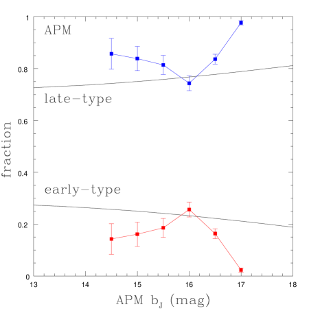
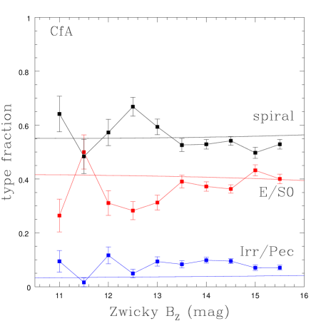
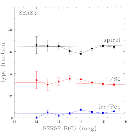
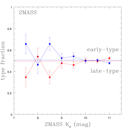
Figure 2: Morphological type fractions as a function of apparent magnitude for the APM (top left), CfA (top right), SSRS2 (lower left) and 2MASS (lower right) surveys. The points with error bars are the data and the curves are the type fractions predicted by the best fit Schechter luminosity functions for the surveys. For the APM survey the relative comoving densities were set to produce the correct average type ratio, as Loveday et al. (1992) did not report the density normalizations for their LFs by type. For the CfA survey, the data we used does not exactly match that fit by Marzke et al. (1994b) in deriving the luminosity function which may lead to differences in the mean comoving densities between the model and the data used here. The CfA and 2MASS survey regions overlap but were independently typed. Note that the features in the type fraction seen for bright magnitudes (which are dominated by the Virgo cluster region) are almost identical. The CfA, 2MASS, and SSRS2 surveys all exhibit morphological type fractions which are, as predicted, roughly constant with apparent magnitude.

We can make a similar comparison for three recent redshift surveys which defined spectral types for the sample galaxies, as shown in Figure 3. Tresse et al. (1999) and Loveday et al. (1999) reanalyzed the APM survey by dividing the sample into bins of low, medium, and high H$\alpha$ (and O[II]) equivalent widths. The spectra were obtained with an 8 arcsec wide long-slit spectrograph which typically covered 45% of the galaxy above the 25 mag/arcsec² isophote (see Tresse et al. (1999)). The LCRS (Shectman et al. (1996)) and ESP (Vettolani et al. (1997)) surveys used fiber spectrographs with fiber diameters of 3$\farcs$5 and 2$\farcs$5 respectively. Both the LCRS (Lin et al. (1996)) and ESP (Zucca et al. (1997)) luminosity functions defined by emission line equivalent widths show strong systematic trends in the type fraction with redshift—the low EW fraction diminishes with redshift while the high EW fraction steadily rises. In the Bromley et al. (1998a) analysis of the LCRS survey, the galaxies were divided into 6 spectral clans (1=earliest, 6=latest) which we have simplified in Figure 3 by combining the clans in pairs since each pair member shows very similar behavior. The earliest pair (clans 1 and 2) shows a steep drop with magnitude, the intermediate pair (clans 3 and 4) shows a compensating rise, and the latest pair (clans 5 and 6) shows no variation. Except for the APM results and the latest clan pair in Bromley et al. (1998a), the variations in the type fractions are in gross disagreement with those predicted from the luminosity function models.

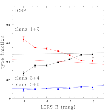
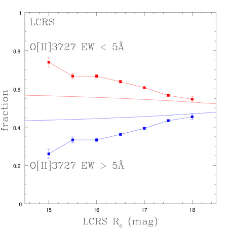
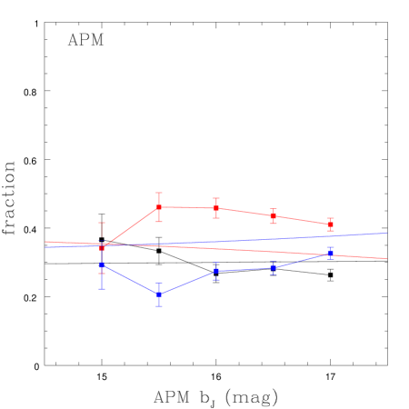
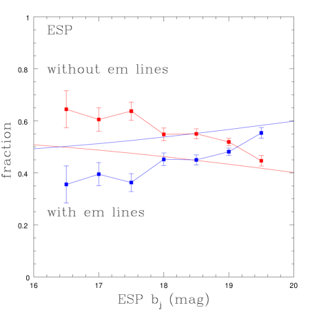
Figure 3: Spectral type fractions as a function of apparent magnitude for the LCRS by spectral clan (top left) and emission line equivalent width (top right), for the APM survey by emission line equivalent width (lower left), and the ESP survey by emission line equivalent width (lower right). The LCRS (classified both by “clans” and [O II] equivalent widths) and ESP surveys, which were all done with fiber-fed spectrographs, show strong dependences of spectroscopic type fractions with apparent magnitude; the APM survey, which was based on large aperture long-slit spectra, does not.

3 The Failure of Spectral Typing

While no survey has type fractions which exactly match the predictions of its luminosity functions, we conclude that morphological classification leads to broadly self-consistent results for bright, nearby galaxy samples (CfA, SSRS2, 2MASS). It can fail badly for more distant, fainter samples like the APM when the images lack sufficient dynamic range or resolution to distinguish successfully among galaxy types. The surprising result is that spectrally-typed samples from fiber surveys (ESP and LCRS) fail the test badly, while the smaller APM sample based on long slit spectra passes the test. Global spectra of galaxies must lead to well-defined, self-consistent spectral type definitions, so the most likely origin of the problem is the small size of the spectral apertures used by the fiber Surveys. At the median redshift ($z\simeq 0.1$) of all the fiber surveys (LCRS, ESP, 2dFGRS, SDSS) the fiber sizes match the typical size of a galactic bulge ($1\farcs 0=1.2h^{-1}$ kpc). In the fiber surveys, an early-type spiral galaxy with a large bulge will have the spectrum of an early-type galaxy when it is bright, nearby, and the fiber covers only the bulge; on the other hand, it will have a later-type spectrum when it is faint, distant, and the fiber includes part of the disk. Such an aperture bias very naturally explains the trends seen for the ESP and LCRS surveys in Figure 3.

Few studies using spectral typing methods have considered the problems of aperture bias. Tresse et al. (1999) discuss the issue for the APM survey, concluding that their 8$\farcs$0 wide longslit aperture is large enough to avoid any biases, as is borne out by our tests in §2. Zaritsky et al. (1995) discuss the issue briefly, concluding that aperture bias would not be a problem. Our own reading of the Zaritsky et al. (1995) tests drives us to the opposite conclusion, at least for the restricted problem of determining luminosity function shapes where differential errors in classifications as a function of luminosity can radically change the derived faint-end slopes. Quantitatively estimating the extent of the problem is difficult because we lack detailed probability distributions for the structural variables describing spiral galaxies (bulge-to-disk luminosity ratios, disk scale lengths, and bulge scale lengths as a function of total luminosity). We can, however, show that the spectral types are ill-defined by comparing the fiber apertures to images of galaxies in §3.1, examining the variation in H$\alpha$ equivalent widths with aperture size in §3.2, and considering simplified models of galaxies in §3.3. In §3.4 we explore some of the consequences of aperture bias for spectrally-typed luminosity functions.

3.1 Evidence for Aperture Bias from Galaxy Images

We start by illustrating the problem with images. Figure 4 shows the 3$\farcs$5 diameter LCRS fiber aperture superposed on POSS II images of Sa and Sb galaxies with a range of absolute luminosities ($-2$ mag to $+2$ mag relative to $L_{*}$ from our 2MASS survey) after rescaling the images to the redshift at which they would have $R_{c}\simeq 16.5$ mag in the LCRS survey. The images make clear that the fiber apertures sample only central spectra and that the region covered by the aperture depends strongly on redshift or apparent magnitude. Even for the faintest LCRS galaxies ($R_{c}\simeq 18$ mag), most of the galaxy disks lie outside the aperture. The aperture problem becomes steadily worse for the SDSS, ESP, and 2dFGRS surveys which have smaller fiber diameters (3$\farcs$0, 2$\farcs$5, and 2$\farcs$0 respectively) but approximately the same median redshift. The biases become smaller for surveys with larger spectrographic apertures, as illustrated by the APM results. Seeing (which will increase the effective fiber aperture by 0$\farcs$5 to 1$\farcs$0 depending on the site and the observing conditions) and pointing/coordinate errors ($\sim 0\farcs 3$ to $1\farcs 0$) will increase the disk fraction entering the fiber, but not by enough to remove the problem. For example, we left the pointing offsets between POSS II and 2MASS in Fig. 4 to provide an indication of their importance. Non-uniformities in the fiber illumination will tend to reduce the effective aperture.

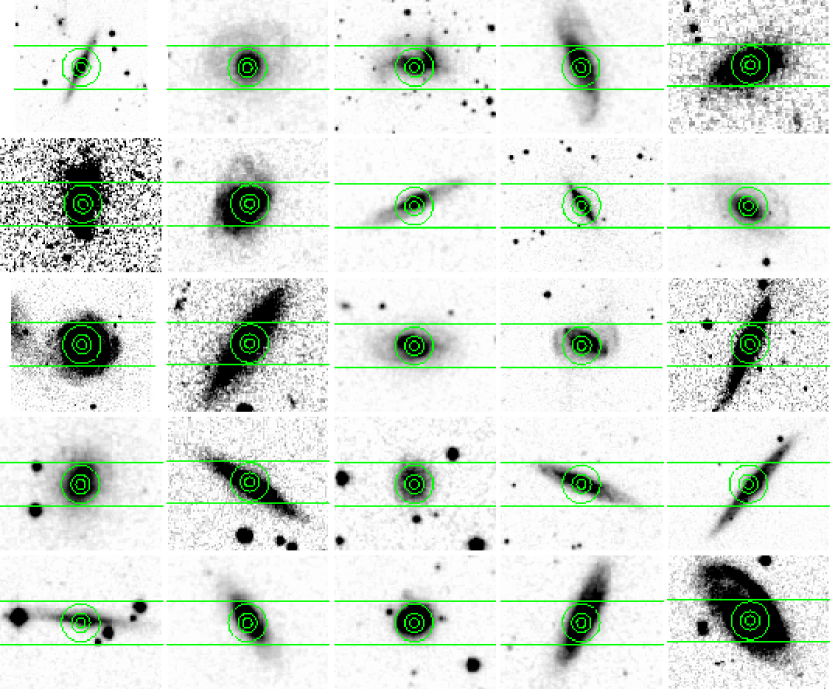
Figure 4: Fiber apertures superposed on galaxies. The greyscale POSS II images are Sa and Sb galaxies from the 2MASS survey rescaled to the redshifts they would have at the midpoint of the LCRS survey ($R_{c}=16.5$ mag). The galaxies in each row have the same absolute luminosity ($-2$, $-1$, $0$, $+1$ and $+2$ mag relative to $L_{*}$ from top to bottom) based on the late-type galaxy infrared luminosity function. The superposed circles show the area covered by the 3$\farcs$5 diameter LCRS fiber aperture at the redshifts corresponding to the galaxy being observed over the magnitude range of the LCRS survey. The offsets are due to astrometry differences between 2MASS and the digitized POSS II images, which we left in to give a feeling for the effects of pointing errors. The largest circle corresponds to the faint limit, $R_{c}=18$ mag, the middle circle to the midpoint $R_{c}=16.5$ mag, and the smallest circle to the bright limit $R_{c}=15$ mag. The ESP, 2dFGRS and SDSS surveys have very similar survey depths but smaller fiber aperture diameters of 2$\farcs$5, 2$\farcs$0 and 3$\farcs$0 respectively. The horizontal lines show the geometry of the APM spectrograph slit at the LCRS midpoint and should be compared in size to the intermediate circle. It is clear that the typical fiber size (intermediate circles) represent incomplete and unrepresentative samples of the light distribution of the galaxies; it would be extremely difficult to classify these galaxies accurately if only the light within the intermediate circles were used. On the other hand, the large rectangular apertures of the APM survey are a far better sampling of the overall galaxy light distributions, and hence classifications based on such spectra are arguably more reliable, accurate, and representative.

3.2 Evidence for Aperture Bias from Galaxy Spectra

We can also illustrate the problem using spectra. We have a large sample of high signal-to-noise ratio, major axis, long slit spectra of 2MASS galaxies in the magnitude range $10.5<K_{s}<11.25$ mag, which were obtained to measure the dynamical properties of a statistically well-defined sample of galaxies. The slit width is 2$\farcs$0. We extracted spectra for slit lengths of 2$\farcs$6, 5$\farcs$2, 10$\farcs$3, 20$\farcs$6 and 41$\farcs$3 (2, 4, 8, 16 and 32 pixels) and computed the H$\alpha$ equivalent width for each aperture. The median redshift of galaxies in this magnitude range is $z\simeq 0.027$ (Kochanek et al. 2000a ) which roughly corresponds to $13.4<R_{c}<14.2$ mag in the LCRS sample if we match the two samples using median redshifts. Galaxies were classified as having central AGN if their emission-line equivalent widths were $\log$[O I]$/\log$H$\alpha>-1.2$ dex or $\log$[N II]$/\log$H$\alpha>-0.25$ dex, which we adapted from Osterbrock (1989) to match those lines available in our spectra. “Star-forming” galaxies were defined as those with detectable H$\alpha$ in all apertures; “intermediate” galaxies were those without H$\alpha$ in one or more apertures. Figure 5 shows that many galaxies with emission lines have equivalent widths which rise with increasing aperture area, although there is also a minority of star-forming galaxies with falling equivalent widths which could be created by emission from a weak central AGN. For illustration we can count the number of galaxies crossing the spectral boundaries used by the APM survey at H$\alpha$ equivalent widths of 2Å  and 15Å. Of the 76 galaxies we studied here, seven (9%) cross from low to intermediate EW, five (7%) cross from intermediate to high EW, seven (9%) cross from intermediate to low EW, and three (4%) cross from high to intermediate EW. In total, 29% of the galaxies change their spectral classification as we increase the slit length. Note that the slopes of many galaxies with decreasing EW become fairly flat for the longer slit lengths, while the slopes of galaxies with increasing EW are often still increasing rapidly for the longer slit lengths.

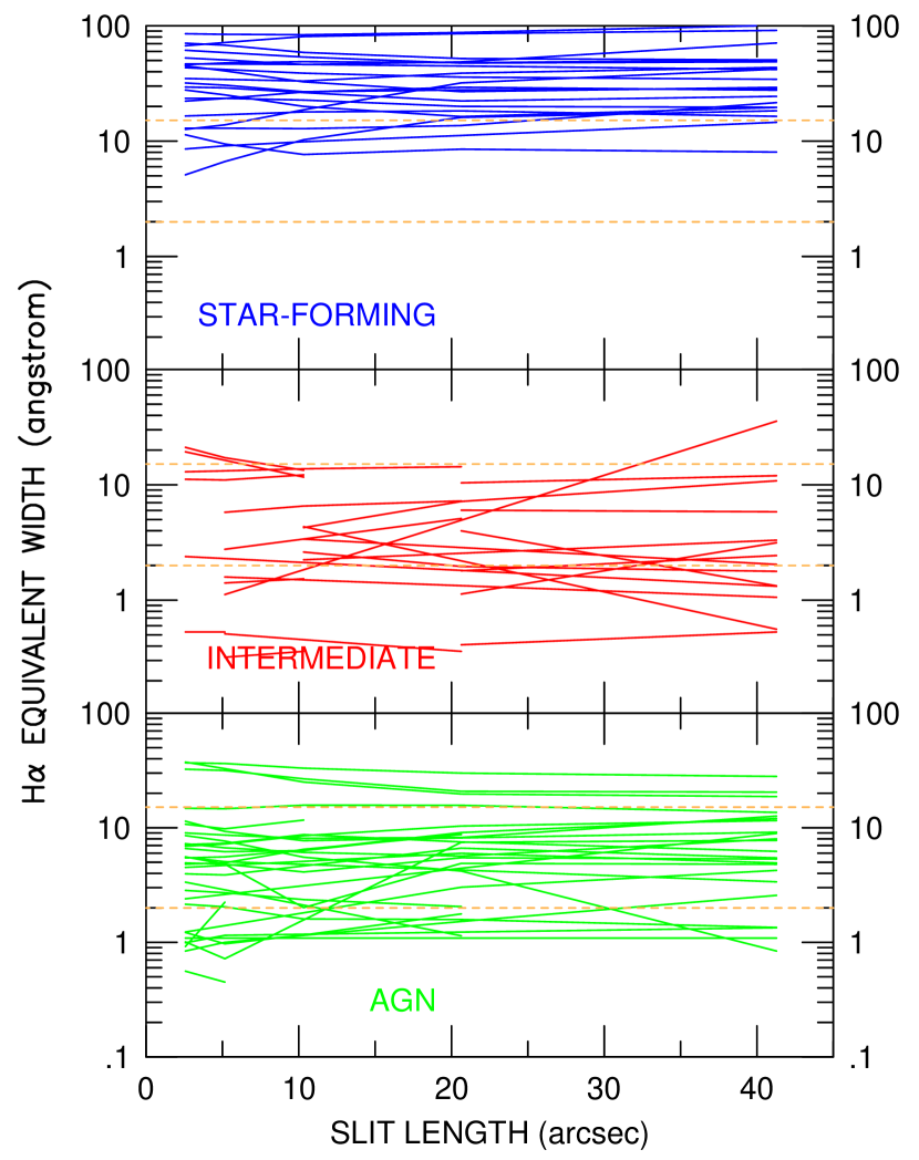
Figure 5: The H$\alpha$ equivalent widths as a function of spectroscopic aperture length for 76 randomly-selected 2MASS galaxies with $10.50<K_{s}<11.25$ mag. The dashed horizontal lines are the spectral type boundaries used by the APM survey. Galaxies were roughly subdivided by spectroscopic type: “AGN” are those galaxies with high [O I]/H$\alpha$ or [N II]/H$\alpha$ in their central aperture; “star-forming” galaxies were those with detectable H$\alpha$ in all extracted apertures; and “intermediate” are those with H$\alpha$ not detected in one or more aperture. A significant percentage of galaxies, with and without AGN, cross the APM type boundaries with increasing spectroscopic aperture, thus demonstrating a potential aperture bias in spectroscopic classification.

Geometry makes it difficult to convert quantitatively our observations into equivalent LCRS observations. Let $r$ be the ratio of the slit length to the fiber diameter. The spectrum of a 2MASS galaxy at redshift $z_{0}$ covers the same area as the LCRS spectrum of a galaxy at redshift $z=0.85z_{0}r^{1/2}$ and it has the same physical length as the LCRS fiber diameter at redshift $z=z_{0}r$. For a face-on galaxy, matching the physical areas of the spectral apertures is the better approximation (although the slit extends further into the disk for the same total area), while for an edge-on galaxy, matching the physical lengths of the spectral apertures is the better approximation. Given that the median redshift of the 2MASS sample is only one-quarter than of the LCRS sample, $r\simeq 20$ corresponds to the median LCRS redshift if we match the physical areas of the apertures and $r\simeq 4$ if we match the physical lengths. Thus, Figure 5 either illustrates the equivalent width trends for the bright LCRS sample, if you match physical areas, or the full LCRS sample, if you match physical lengths.

Figure 5 also illustrates the dangers of subdividing the sample into large numbers of spectral types. While only 29% of the galaxies would cross the APM boundaries dividing the sample into three types, a higher percentage would cross sample boundaries if we divide the sample into five types by adding another boundary at 5Å. Larger numbers of classes lead to lower reliability because larger fractions of the galaxies of a particular type are actually galaxies drifting through that type due to the effects of aperture bias rather than galaxies which intrinsically have that spectral type.

3.3 Evidence for Aperture Bias from Galaxy Models

Finally, the problem can be illustrated with simple models. We phrase the discussion in terms of emission line equivalent widths, but the same effects will be found in more sophisticated principal component analyses or galaxies typed based on broad band colors measured in small apertures. Consider a face-on galaxy composed of an exponential disk (scale length $h_{d}$) and a de Vaucouleurs bulge (effective radius $R_{e}$) with a bulge-to-disk luminosity ratio of $B/D$. The average relation between the two scale lengths is $\log R_{e}=0.95\log h_{d}-0.86$ ($\pm 50\%$) for the K-band, but the scatter increases steadily towards shorter wavelengths (de Jong (1996)). We assume that the spectrum of the disk includes an emission line with equivalent width $EW_{0}$ while the bulge has no emission lines, so that the global spectrum of the galaxy would have equivalent width $EW_{g}=EW_{0}/(1+B/D)$ because the addition of the continuum from the bulge reduces the equivalent width of the disk emission line. In a finite radius spectral aperture $\theta$ ($1\farcs 75$ for LCRS), we collect fractions $f_{D}(\theta D_{A}(z)/h_{d})$ and $f_{B}(\theta D_{A}(z)/R_{e})$ of the light from the disk and the bulge respectively, where $D_{A}(z)$ is the angular diameter distance to the galaxy. We then observe an emission line equivalent width of

$$EW_{obs}=EW_{0}\left[{1\over 1+(f_{B}/f_{D})(B/D)}\right]=EW_{g}\left[{1+B/D\over 1+(f_{B}/f_{D})(B/D)}\right],$$ (3)

which differs from the global value of the equivalent width. Spectral types will be inconsistent if the ratio $EW_{obs}/EW_{g}$ strongly on the intrinsic or extrinsic properties of the galaxy, and they will be biased if the ratio depends on luminosity.

As we qualitatively predicted based on Figures 4 and 5, the spectral properties of the galaxies as traced by the variations in $EW_{obs}/EW_{g}$ depend strongly on the distance to the galaxy. Figure 6 shows the expected changes in $EW_{obs}/EW_{g}$ for galaxies with disk scale lengths of $h_{d}=3h^{-1}$ kpc and $0.5h^{-1}$ kpc and a range of bulge-to-disk ratios from 5% to 30% assuming the mean bulge scale length from de Jong (1996) and the LCRS fiber aperture. We assumed that the $3h^{-1}$ kpc galaxy was an $L_{*}$ galaxy with $M_{R}=-20.3$ mag and that the disk surface brightness was independent of luminosity so that the $h_{d}=0.5h^{-1}$ kpc galaxy has $M_{R}=-16.4$ mag. The larger the bulge-to-disk ratio, the larger the fractional changes in the ratio over the redshift range for which the galaxy would be included in the survey. For a galaxy with $B/D=0.2$, a galaxy with an intrinsic equivalent width of $EW_{g}=10$Å  would be classified as low equivalent width ($EW<5$Å  in Lin et al. (1996)) over half the survey’s magnitude range, and the equivalent width is well below the true, global value at all magnitudes. This is, of course, a simplified example. Some early-type spirals show no emission lines along the line-of-sight through the bulge, which would exacerbate the effect. Edge-on galaxies would have a larger fraction of the disk light in the aperture if they were transparent but might not if we include dust. Qualitatively, however, aperture bias naturally produces the decreasing early-type and rising late-type galaxy fractions as a function of apparent magnitude in the LCRS and ESP surveys.

3.4 Consequences of Aperture Bias for Luminosity Functions

It is more difficult to determine whether the spectral types and the luminosity function are biased because of the sensitivity of the problem to so many parameters. The simplest mathematical description of the problem, neglecting inclination and extinction, starts from the distribution of galaxies in luminosity, spectral type (as represented by the global equivalent width) and structural properties ($h_{d}$, $R_{e}$ and $B/D$), $dn/dLdEW_{g}dh_{d}dR_{e}d(B/D)$. We want to derive the distribution in luminosity and spectral type

$${dn\over dLdEW_{g}}=\int dh_{d}dR_{e}d(B/D){dn\over dLdEW_{g}dh_{d}dR_{e}d(B/D)},$$ (4)

but we actually measure $EW_{obs}$ to obtain

$${dn\over dLdEW_{obs}}=\int dh_{d}dR_{e}d(B/D){dn\over dLdEW_{g}dh_{d}dR_{e}d(B/D)}{1+B/D\over 1+(B/D)(f_{B}/f_{D})}.$$ (5)

where the correction factor is the ratio from eqn. (3) and illustrated in Fig. 6. We can simplify and illustrate the problem by assuming that the scale lengths are simple power laws of the luminosity, $h=h_{0}(L/L_{0})^{\beta}$ and $R_{e}=R_{0}(L/L_{0})^{\gamma}$, so that

$${dn\over dLdEW_{obs}}=\int d(B/D){dn\over dLdEW_{g}d(B/D)}{1+B/D\over 1+(B/D)(f_{B}/f_{D})}$$ (6)

where the arguments for the curve of growth functions have the form $\theta D_{A}(z)/h_{0}(L/L_{0})^{\beta}$. In a Euclidean universe (which is almost correct locally), a source of flux $F$ and luminosity $L$ is seen at distance $D_{A}(z)=(L/4\pi F)^{1/2}$, so the arguments for the curve of growth functions have the form, $\theta(F/F_{0})^{-1/2}(L/L_{0})^{1/2-\beta}$ where $F_{0}=L_{0}/4\pi h_{0}^{2}$. For self-similar galaxies, defined by $\beta=\gamma=1/2$, the arguments become independent of luminosity and depend only on the flux. This flux dependence is sufficient to explain the problems in current spectral classifications. Self-similar galaxies also have self-similar surface brightness profiles with constant central surface brightnesses. The de Jong (1996) mean K-band relation between the disk and bulge scale lengths satisfies $\beta\simeq\gamma$ since $R_{e}\propto h_{d}^{0.95}$, but the scatter is large and the relations for constant $EW_{g}$ and $B/D$ could differ from the relation averaged over these variables. The value of $\gamma$ is more problematic since it is closely related to the problem of surface brightness completeness in surveys (e.g. Dalcanton (1998)). In standard bright galaxy samples, all disks have similar central surface brightnesses (even if it is a selection effect!) suggesting that $\beta\simeq 0.5$. Unfortunately, the calculation is extraordinarily sensitive to the value of $\beta$, as illustrated Figure 7 by using $\beta=0.4$, $0.5$, and $0.6$ to scale the properties of the smaller galaxy from Figure 6. In short, aperture biases are almost certainly luminosity dependent, but we cannot prove (or disprove) it from the available statistical data on the structural properties of spiral galaxies.

Figure 6: The ratio of the measured to the global emission line equivalent width as a function of redshift for observations scaled to resemble the LCRS survey. The bulge-to-disk ratios are 5%, 10%, 20% and 30% from top to bottom and the lines are plotted for the redshift range over which the galaxies would have $15<R_{c}<18$ in the LCRS survey. The aperture bias in measured equivalent width is a strong function of scale-length, bulge-to-disk ratio, and redshift.

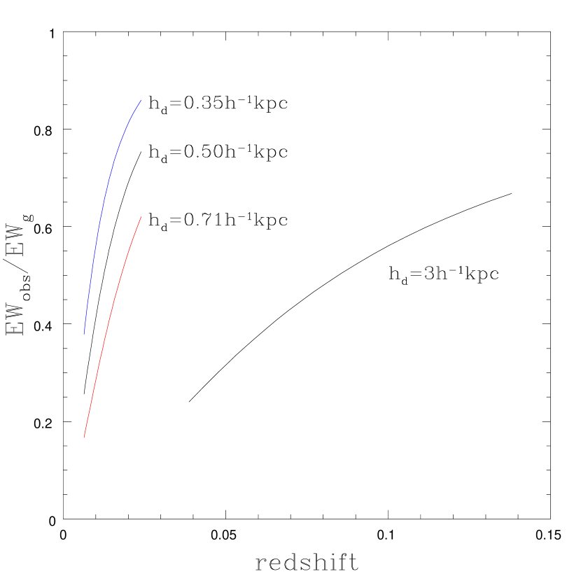
Figure 7: Effect of deviations from self-similar surface brightness profiles. We show the ratio of the observed and intrinsic equivalent widths for the $B/D=0.2$ case from Figure 6, but for the small galaxy we show the results of scaling the disk radius with luminosity as $h\propto L^{\beta}$ with $\beta=0.6$ ($h_{d}=0.35h^{-1}$ kpc), the self-similar exponent $\beta=0.5$ ($h_{d}=0.50h^{-1}$ kpc), and $\beta=0.4$ ($h_{d}=0.71h^{-1}$ kpc) corresponding to a change in the mean surface brightness by $\pm 0.75$ mag/arcsec² for a 3.9 mag change in the luminosity.

The most likely effect of aperture bias is to misclassify fraction $f(M)$ of spectrally late-type galaxies as early-type galaxies, and we can use this to explore the sensitivity of spectrally-typed luminosity functions to its effects. The observed luminosity functions are

$$\phi_{E}^{obs}(M)=\phi_{E}(M)+f(M)\phi_{L}(M)\qquad\hbox{and}\qquad\phi_{L}^{obs}(M)=\left[1-f(M)\right]\phi_{L}(M)$$ (7)

rather than the true luminosity functions $\phi_{E}(M)$ and $\phi_{L}(M)$, but we can easily invert the equation given a model for the error rate $f(M)$. Lets initially consider the case where $f(M)=f$ is a constant. The consequences of the errors then depend on the relative shapes of the luminosity functions. If the shapes of the luminosity functions are similar, then the only effect is to adjust the comoving density estimates. For example, when we examined the effects of typing errors on the morphologically-typed luminosity functions for the 2MASS survey, we found almost no effect due to random typing errors and only slow parameter drifts from typing biases (see Kochanek et al. 2000a ); this effect is a direct result of the roughly constant numbers of galaxies of each morphological type near to the boundary between early- and late-type galaxies (S0/a). The consequences of both random and systematic errors are far greater when the shapes of the luminosity functions are very different, as is found in the spectrally-typed surveys. Figure 8 illustrates the problem for the Schechter function models of the high and low equivalent width samples from Lin et al. (1996). Where the late-type galaxies dominate the comoving density, small ($f=5\%$!) classification problems for the late-type galaxies strongly modify the shape of the early-type luminosity function. Even for purely random errors in the galaxy types, Malmquist bias can mean that the observed density of the rarer galaxy type is dominated by misclassified galaxies of the common type. Large, luminosity dependent biases are needed to make the early-type slope flatter and more similar to the late-type slope or the results of the morphological surveys. Crudely, a $f(L_{*})=30\%$ error rate is enough to reduce the density of low EW galaxies near $L_{*}$ by a factor of two, which must be combined with a rapid reduction in the error for fainter galaxies so that $f(L_{*}/10)\simeq 0$. The corrected luminosity function which results from such a bias has a flat faint-end slope. Whether the actual biases can achieve this is unknown.

Figure 8: Effect of unbiased misclassification on the LCRS luminosity functions divided by O[II]3727Å  equivalent width. The solid curves are the parameterized luminosity functions for high ($>5$Å) and low ($<5$Å) EW from Lin et al. (1996). The dashed lines show the intrinsic luminosity functions assuming that $f=$5%, 10%, or 20% of the intrinsically high EW galaxies are misclassified as low EW galaxies because of aperture bias independent of luminosity (the self-similar case). Small misclassification rates lead to enormous changes in the intrinsic luminosity function of the low EW galaxies because the high and low EW luminosity functions are so different.

The differences between the measured and global spectra affect not only the luminosity functions, but also applications of the spectrally-typed surveys to other problems. For example, Blanton (2000, also see Tegmark & Bromley (1999)) had already discovered inconsistencies in estimates of type-dependent cosmological biasing parameters from the LCRS survey when the sample was divided into high and low redshift samples. Blanton (2000) found that surface brightness selection effects were probably not the origin of the problem, and suggested spectral typing problems as an alternative. Bromley et al. (1998b) extended their earlier survey (Bromley et al. 1998a ) to estimate the luminosity function by clan in high and low density environments. They found that the luminosity functions of the clans most sensitive to the aperture biases (clans 1–4) show stronger dependences on environment than those which are less sensitive (clans 5–6). The sense of the difference, that the early-type clans in the low density, late-type rich environment showed still larger faint-end slope differences than the sample as a whole, is exactly the effect expected from typing biases in which spectrally late-type galaxies are systematically misclassified as early-type galaxies. Where the late-type galaxy fraction is larger, the bias should be larger. The aperture sizes are also small enough to affect estimates of global star formation rates based on the emission lines at all redshifts in the survey. These may affect studies of the differences in star formation rates in different environments (e.g., Hashimoto et al. (1998), Allam et al. (1999)) because the classification error rate depends on environment. These particular studies minimized any biases by comparing galaxies with similar central concentrations to their luminosity profiles.

Figure 9: The ratio of the measured to the global emission line equivalent width for galaxies with bulge-to-disk ratios of 10% (solid) and 30% (dashed) viewed through effective aperture diameters of (bottom to top) 3$\farcs$5, 7$\farcs$0, 10$\farcs$5, and 14$\farcs$0. The scalings are the same as in Figures 6 and 7.

4 What Can Be Done?

The lure of spectral typing—that it supplies a fast, quantitative method for dividing galaxy samples into types—proves to be chimerical in its practical application because the precisely measured spectral types have an unknown, but inconsistent and biased, relation to the true spectral types. We predict that the problems demonstrated in §2 for the LCRS and ESP surveys will also be found in the 2dFGRS and SDSS surveys, since the fiber apertures and mean redshifts of the four surveys are all comparable. Morphological classification appears to avoid such biases for nearby galaxy samples (CfA, SSRS2, 2MASS), but is difficult to extend to the redshift range or sample sizes of the deeper surveys. In this section we discuss methods for correcting current spectral typing systems and alternative typing strategies.

The simplest solution to the problem would be to measure the global spectra of the galaxies. For fiber spectrographs this is easy to implement by dithering the position of the instrumental guide stars rather than holding them fixed during the integration. The required dither amplitude is surprisingly large. Figure 9 shows the ratio between the true and global equivalent widths (as in Figs. 6 and 7) for effective aperture diameters of 3$\farcs$5 (the LCRS aperture), 7$\farcs$0, 10$\farcs$5 and 14$\farcs$0. Apertures two to three times larger than the LCRS aperture (i.e. comparable in size to the APM aperture) are needed to minimize the effects of aperture bias on spectral types. Unfortunately, longer integrations are required because the continuum signal-to-noise ratio of the observations scales as the mean surface brightness of the galaxy inside the dithered aperture (assuming the noise is dominated by the sky brightness), and for typical fiber sizes, the integration time for fixed signal-to-noise initially scales roughly as the aperture diameter. The signal-to-noise ratio for emission lines may actually be larger with dithering because the equivalent width of the emission lines rises with the increase in aperture size.

If measuring the global spectra of all galaxies is impossible, global spectra can be measured for a random sub-sample of the galaxies to build a statistical model for the effects of aperture bias. Enough spectra are required to build a contingency table for converting survey spectral types into global spectral types. Since a three-dimensional table is required (the global spectral type as a function of the survey spectral type and the apparent magnitude), the global spectra of $\sim 10^{3}$ galaxies are needed to provide adequate statistics. Nonetheless, for large redshift surveys with $10^{5}$-$10^{6}$ galaxies, the overhead required to measure $10^{3}$ global spectra is only 1-10% of the total survey even if the integration times are 10 times longer. This sampling method also has the advantage that it can be applied retroactively to an existing survey.

Rather than obtaining global spectra, a survey can try to obtain “isophotal” spectra for survey fields that require multiple exposures (more objects than fibers). The targets are divided into isophotal radius bins and the effective aperture (the amount of dithering) is scaled by the isophotal radius. Perfect isophotal spectra avoid redshift and flux dependent changes in the spectral types of galaxies with the same intrinsic properties. Thus, isophotal spectra provide self-consistent galaxy types, although there will still be luminosity and structure dependent differences between the isophotal and global spectra. By choosing the isophotes and effective apertures so that they match the fiber size for the faintest galaxies, the overhead of obtaining “isophotal” spectra is minimized because large dithers are required only for the brighter, nearby galaxies. Instead of the rapid redshift variations in the ratio of the measured to global equivalent widths seen in Figs. 6, 7, and 9, the ratios found for isophotal spectra would be nearly independent of redshift.

Surveys based on modern multi-color CCD photometry (SDSS and, to a lesser extent, 2MASS) should probably type galaxies based on either broad band colors or fits to the luminosity profiles of the galaxies (e.g. concentration or bulge-to-disk ratio). While colors lack the physical precision of spectra, it is relatively simple to avoid redshift-dependent changes in the type-boundaries. Colors are not free of biases, as dust creates strong, inclination dependent variations in the colors of late-type galaxies. Of the surveys we discuss, only the SDSS survey can easily define galaxy types based on broad band colors. Most of the other surveys have no color information or have only low precision photographic colors (APM, CfA, ESP, LCRS, SSRS2, and 2dFGRS), while the infrared colors measured by the 2MASS survey have little sensitivity to galaxy type. One-dimensional light profile fits are the remaining possibility for automatically assigning galaxy types. These may be the most reliable means of typing galaxies, but they are difficult to automate. In particular, all superposed stars and galaxies must be identified and masked before performing the necessary profile fitting. Like morphological typing, profile typing requires good resolution and high dynamic range images.

In summary, all galaxy classification methods suffer from systematic errors and biases. We are relatively familiar with those of morphological classification, but no method is immune to the problem. In particular, the application of spectral typing to large redshift surveys can be easily automated and “objective” while still introducing significant systematic biases and uncertainties. Because of the shear size of modern redshift surveys, these systematic errors are more important than statistical errors and thus require careful attention in both the planning and analysis of such surveys.

References

- Allam et al. (1999) Allam, S.S., Tucker, D.L., Lin, H., & Hashimoto, Y. 1999, ApJL, 522, L89
- van den Bergh et al. (1996) van den Bergh, S., Abraham, R. G., Ellis, R. S., Tanvir, N. R., Santiago, B. X., & Glazebrook, K. G. 1996, AJ, 112, 359
- Binggeli, Sandage, & Tammann (1988) Binggeli, B., Sandage, A., & Tammann, G.A. 1988, ARA&A, 26, 509
- Blanton et al. (1999) Blanton, M., Cen, R., Ostriker, J. P., & Strauss, M. A. 1999, ApJ, 522, 590
- Blanton (2000) Blanton, M. 2000, ApJ, in press (astro-ph/0003228)
- (6) Bromley, B.C., Press, W.H., Lin, H., & Kirshner, R.P. 1998a, ApJ, 505, 25
- (7) Bromley, B.C., Press, W.H., Lin, H., & Kirshner, R.P. 1998b, ApJ, submitted (astro-ph/9805197)
- Connolly et al. (1995) Connolly, A.J., Szalay, A.S., Bershady, M.A., Kinney, A.L, & Calzetti, D. 1995, AJ, 110, 1071
- da Costa et al. (1998) da Costa, L.N., et al. 1998, AJ, 116, 1
- Dalcanton (1998) Dalcanton, J. J. 1998, ApJ, 495, 251
- de Jong (1996) de Jong, R.S. 1996, A&A, 313, 45
- van Dokkum & Franx (1996) van Dokkum, P. G., & Franx, M. 1996, MNRAS, 281, 985
- Dressler (1980) Dressler, A. 1980, ApJ, 236 351
- Dressler et al. (1997) Dressler, A., Oemler, A., Jr., Couch, W. J., Smail, I., Ellis, R. S., Barger, A., Butcher, H., Poggianti, B. M., & Sharples, R. M., 1997, ApJ, 490, 577
- Folkes et al. (1999) Folkes, S., et al. 1999, MNRAS, 308, 459
- Hashimoto et al. (1998) Hashimoto, Y., Oemler, A., Lin, H., & Tucker, D.L. 1998, ApJ, 499, 589
- Hubble (1936) Hubble, E. P. 1936, The Realm of the Nebulae (New Haven: Yale Univ. Press)
- Kochanek (1996) Kochanek, C. S. 1996, ApJ, 466, 638
- (19) Kochanek, C. S., Pahre, M. A., Falco, E. E., Huchra, J. P., Mader, J., Jarrett, T., Chester, T., Cutri, R., & Schneider, S. 2000a, ApJ submitted
- (20) Kochanek, C. S., Falco, E. E., Impey, C. D., Lehar, J., McLeod, B. A., Rix, H.-W., Keeton, C. R., Munoz, J. A., & Peng, C. Y. 2000b, ApJ, 543, 131
- Kolatt & Dekel (1997) Kolatt, t., & Dekel, A. 1997, ApJ, 479, 592
- Lilly et al. (1995) Lilly, S. J., Tresse, L., Hammer, F., Crampton, D., & Le Fèvre, O. 1995, ApJ, 455, 108
- Lin et al. (1996) Lin, H., Kirshner, R.P., Shectman, S.A., Landy, S.D., Oemler, A., Tucker, D.L., & Schechter, P.L. 1996, ApJ, 464, 60
- Loveday et al. (1992) Loveday, J., Peterson, B.A., Efstathiou, G., & Maddox, S.J. 1992, ApJ, 390, 338
- Loveday et al. (1996) Loveday, J., Peterson, B.A., Efstathiou, G., & Maddox, S.J. 1996, ApJS, 107, 201
- Loveday, Tresse, & Maddox (1999) Loveday, J., Tresse, L., & Maddox, S. 1999, MNRAS, 310, 281
- (27) Marzke, R.O., Geller, M.J., Huchra, J.P., & Corwin, H.G. 1994b, AJ, 108, 437
- Marzke et al. (1998) Marzke, R.O., da Costa, L.N., Pellegrini, P.S., Willmer, C.N.A., & Geller, M.J. 1998, ApJ, 503, 617
- Morgan & Mayall (1957) Morgan, W. W., & Mayall, N. V. 1957, PASP, 69, 291
- (30) Naim, A., Lahav, O., Sodre, L., & Storrie-Lombardi, M.C. 1995a, MNRAS, 275, 567
- (31) Naim, A., et al. 1995b, MNRAS, 274, 1107
- Oemler (1974) Oemler, A., Jr. 1974, ApJ, 194, 1
- Osterbrock (1989) Osterbrock, D. E. 1989, Astrophysics of Gaseous Nebulae and Active Galactic Nuclei (Mill Valley: University Science Books)
- Sandage & Tammann (1987) Sandage, A., & Tammann, G. A. 1987, A Revised Shapley-Ames Catalog of Bright Galaxies, Carnegie Institution of Washington Publication # 635 (Washington: Carnegie Institution)
- Sandage (1961) Sandage, A. 1961, The Hubble Atlas of Galaxies, Carnegie Institution of Washington Publication # 618 (Washington: Carnegie Institution)
- Schechter (1976) Schechter, P. 1976, ApJ, 203, 297
- Shectman et al. (1996) Shectman, S.A., Landy, S.D., Oemler, A., Tucker, D.L., Lin, H., Kirshner, R.P., & Schechter, P.L. 1996, ApJ, 470, 172
- Slonim et al. (2000) Slonim, N., Somerville, R., Tishby, N., & Lahav, O. 2000, MNRAS, submitted (astro-ph/0005306)
- Stewart (1964) Stewart, P. 1964, concurring opinion in Jacobellis versus Ohio, 378US184, 1964.
- Tegmark & Bromley (1999) Tegmark, M., & Bromley, B. 1999, ApJ, 518, L69
- Tresse et al. (1999) Tresse, L., Maddox, S., Loveday, J., & Singleton, C. 1999, MNRAS, 310, 262
- Vettolani et al. (1997) Vettolani, G., et al. 1997, 325, 954
- Vogt et al. (1996) Vogt, N. P., Forbes, D. A., Phillips, A. C., Gronwall, C., Faber, S. M., Illingworth, G. D., & Koo, D. C. 1996, ApJ, 465, L15
- Zaritsky, Zabludoff, & Willick (1995) Zaritsky, D., Zabludoff, A.I., & Willick, J.A. 1995, AJ, 110, 1602
- Zucca et al. (1997) Zucca, E., et al. 1997, A&A, 326, 477