Comparative CMBology: Putting Things Together
Abstract
I present a series of diagrams which illustrate why the cosmic microwave background (CMB) data favor certain values for the cosmological parameters. Various methods to extract these parameters from CMB and non-CMB observations are forming an ever-tightening network of interlocking constraints. I review the increasingly precise constraints in the plane and show why more cosmologists now prefer CDM cosmologies to any other leading model.
School of Physics, University of New South Wales, Sydney, Australia
charley@bat.phys.unsw.edu.au
1. What is the CMB data trying to tell us?
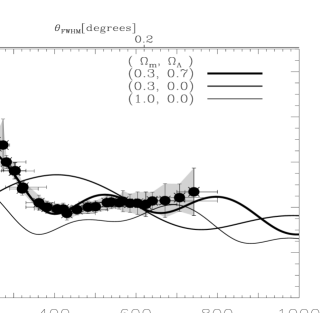
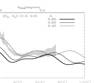
A convenient way to interpret CMB observations is to fit the angular power spectrum of the data to parameter-dependent models. Figure 1 shows the recent CMB measurements along with three such models. In Figure 2, binning of this data reduces the scatter and provides a representative region favored by the data. Important parameters that can be constrained by CMB power spectra include Hubble’s constant , the cosmological constant , the density of cold dark matter , and the density of baryonic matter . Figures 1 - 8 provide a qualitative feel for the lever arm that the CMB data provides for constraining these and other parameters simultaneously. Unless stated otherwise, the models shown have the following default values: , , , , a power spectral index of primordial scalar density fluctuations and an overall normalization K. The grey band in Figure 2 is reproduced in Figures 3 - 8 and represents the data in a model-independent way. With it, the eye can pick out which models best fit the data.
A reduction in increases the amplitude of the first peak (Fig. 3). An increase in the number of baryons increases the gravitating mass of the oscillating baryon-photon fluid . This enhances the first peak (Fig. 4) by producing more gravitational compression as the baryons drag the photons further into the potential wells (and further away from the potential hills). The second peak is suppressed because, before decoupling, these smaller scales experienced the same additional compression (and rarefaction) and, at decoupling, we are seeing a subdued rebound from this enhanced compression (and rarefaction), i.e., we are seeing the smaller amplitude of an oscillation whose zero level had been lowered in the previous oscillation by the effect of additional baryons. An increase in decreases the amplitude of the first peak (Fig. 6). For discussion of the physics of the parameter dependencies of features in the CMB power spectrum see e.g. Hu & Sugiyama (1995), Hu (1995), Tegmark (1996), Lineweaver et al. (1997).



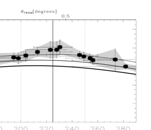
Just as the SNIa data is our strongest lever arm for determining the acceleration of the universe, , the CMB data is our strongest lever arm for determining the geometry of the universe, . The ability of the CMB to constrain can be seen in Fig. 9, panel A and Fig. 10 in which the CMB contours are elongated in the constant direction (upper left to lower right). However, since both and control the position of the peak, there is a slight degeneracy. It is difficult to separate the effect of the spatial geometry of the universe from the effect of . This degeneracy is reflected in the width of the elongated CMB constraints in the plane. The models in Fig. 8 have , . The data and the high baryon model peak at . This crude eye-ball estimate should be compared to the more careful but model-dependent estimates of Bond et al. (2001, ) and Hu et al. (2001, at the level based on the Boomerang and Maxima results only).
2. Putting It All Together
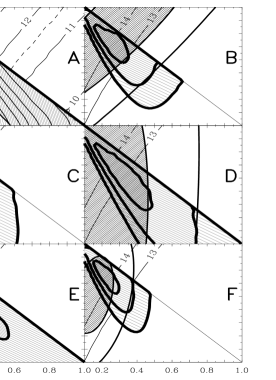
Presumably we live in a universe which corresponds to a single point in multidimensional parameter space. If the universe is to make sense, independent determinations of , , and the minimum age of the Universe must be consistent with each other (Fig. 11). Estimates of from HST Cepheids and from the CMB must overlap. Deuterium and CMB determinations of should be consistent (Fig. 4, but see Kaplinghat & Turner 2000). Regions of the plane favored by SNIa and CMB must overlap with each other and with other independent constraints. That this is the case is shown in Fig. 9.
2.1. Consistency enforcement: a worked example in the plane
If any model can squeak by the SNIa constraints it is the very low models. However these models are the ones most strongly excluded by the CMB data (Fig. 9, panels A & B). The SNIa results show that the universe is accelerating but cannot yield a value of the cosmological constant unless one assumes that the universe is flat. However, that assumption is not necessary since we have CMB data that tells us that the universe is approximately flat. Figure 9 is an example of how various independent constraints can be combined with CMB constraints in the plane. The 2 combined constraints in panel F are limited to open and flat models and are reproduced in Fig. 10.
All four constraints in Fig. 10 come from CMB constraints assuming adiabatic initial conditions, in combination with SNIa constraints. The amplitude () and shape () of the local power spectrum of galaxies were included as additional constraints by Bridle et al. (2000, catalogue of peculiar velocities), Tegmark et al. (2000, IRAS PCSz) and Jaffe et al. (2000, where the first errorbar is the Gaussian prior and the second is the full range considered). To constrain and , marginalization of the other parameters was done by maximization (Lineweaver 1999, Tegmark et al. 2000) and integration (Bridle et al. 2000, Jaffe et al. 2000). The number of parameters marginalized over to obtain the results shown in Fig. 10 is given in Table 1 along with the priors used for , and geometry. Calibration errors were treated slightly differently.

| Reference | Data | # parameters | Geometry | ||
|---|---|---|---|---|---|
| Lineweaver(1999) | pre 4/1999 | 6 | flat open | ||
| Jaffe et al.(2000) | DMR+Boom+Max | 7 | flat open closed | ||
| Bridle et al.(2000) | all | 3 | flat | ||
| Tegmark et al.(2000) | all | 10 | flat open closed |
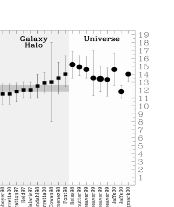
3. The New Standard Model
The parameters that we are trying to determine are fundamental because they give the answers to fundamental questions: What is the universe made of? How old is the universe? How big is the observable universe? My view of the best current values are given in Table 2.
| Parameter estimate | References |
|---|---|
| Fig. 10 | |
| Fig. 10 | |
| Mould et al 99, Parodi et al 00, Freedman et al 01 | |
| Gyr | Fig. 11 |
| Olive et al 99, Tytler et al 01 |
In this paper entitled ‘putting things together’ I have left out a lot: tensor modes (), early reionization (), hot dark matter (, do neutrinos have a cosmologically significant mass), non-Gaussianity, topological defects, quintessence, scale dependent slopes (), non-adiabatic initial conditions, variation in the speed of light and/or the fine structure constant. Any or all of these, or some we have not thought of, may prove to be crucial in the high precision future of CMBology.
3.1. CDM! Any objections?
Lensing constraints in the plane have been invoked as evidence against CDM models (e.g. Kochanek 1996). However in his contribution to these proceedings based on the JVAS/CLASS survey, Helbig reports new lensing constraints which do not exclude the model.
Numerical simulations of the central density profiles of low surface brightness galaxies in CDM models do not match the observations very well, but this may be the result of our ignorance of how baryons assemble into galaxies (Navarro & Steinmetz 2001).
Some cosmologists believe there may be a coincidence problem. Why just now should we have ? (e.g. Carroll 2001, Fig. 11). However, this ‘coincidence’ may well be explained away as an anthropic selection effect.
Another problem with CDM is that it is an observational result that has yet to be theoretically confirmed. From a quantum field theoretic point of view, presents a huge problem and even ‘seems ridiculous’ (Carroll 2001, Sect. 1.3, see also Cohn 1998 and Sahni & Starobinsky 1999). But if observations continue to yield some imaginative theorist will solve this problem.
As more cosmological data comes in, the CMB and non-CMB constraints form an ever-tightening network of interlocking constraints. Fig. 9 shows some of the pieces of this ever-tightening network while Fig. 10 shows the latest tightenings. One of the major new unsung results of recent efforts to simultaneously fit parameters is that the fits are good fits. The parameter values are consistent with each other. This may not last. If, as our data gets better, the best fit model is no longer a good fit, new ideas would be needed. Parameter space may need another few dimensions to contain the real universe. I know of no better way to find these new dimensions than to analyse the increasing precise measurements of the CMB and combine the results with other independent cosmological observations. New data from Boomerang, Maxima, CBI, DASI, VSA, MAP, Beast, Planck and others ensure the health and guarantee continued progress towards determining the fundamental parameters of our universe.
References
- Binney et al 2000 Binney, J., Dehnen, W., & Bertelli, G. MNRAS, submitted, 2001, astro-ph/0003479
- Bond et al 2001 Bond, J.R. et al. 2001, these proceedings, astro-ph/0011378
- Bridle et al. 2000 Bridle, S.L., Zehavi, I., Dekel, A, Lahav, O., Hobson, M.P., Lasenby,A.N. 2000, MNRAS astro-ph/0006170
- Carretta et al. 2000 Carretta, et al. 2000, ApJ, 533, 215
- Carroll 2000 Carroll, S.M. 2001, Living Reviews of Relativity, submitted, Fig. 11, astro-ph/0004075
- Cohn 1998 Cohn, J.D. 1998, Astrophys. Sp. Sci 259, 213, astro-ph/9807128
- Efstathiou et al. 1999 Efstathiou, G., Bridle, S.R., Lasenby, A.N., Hobson, M.P., Ellis, R.S. 1999, MNRAS, 303, L47-L52
- Freedman et al 2001 Freedman, W. et al. 2001, in preparation (these proceedings?)
- Helbig 2001 Helbig, P. 2001, these proceedings, astro-ph/0011031
- Hu 1995 Hu, W. 1995, PhD thesis, Berkeley
- Hu & Sugiyama 1995 Hu, W. & Sugiyama, N. 1995, ApJ, 444, 489
- Hu et al. 2000 Hu, W., Fukugita, M., Tegmark, M. 2001, ApJ, submitted
- Jaffe etal. 2000 Jaffe, A. et al. 2000, PRL, in press, astro-ph/0007333
- Kaplinghat & Turner 2000 Kaplinghat, M. & Turner, M.S. submitted, astro-ph/0007452
- Kochanek 1996 Kochanek, C. 1996, ApJ, 466, 638
- Lineweaver etal 1997 Lineweaver, C.H. et al. 1997, A&A, 322, 365, Section 3.2.1
- Lineweaver & Barbosa 1998 Lineweaver, C.H. & Barbosa, D. 1998, ApJ, 496, 624
- Lineweaver 1998b Lineweaver, C.H. 1998, ApJ, 505, L69
- Lineweaver 1999 Lineweaver, C.H. 1999, Science, 284, 1503-1507
- Mould 1999 Mould, J. et al. 1999, astro-ph/9909260
- Navarro & Steinmetz 2001 Navarro, J. F. & Steinmetz, M. 2001, ApJ, submitted, astro-ph/0001003
- Olive 1999 Olive, K.A., Steigman, G. & Walker, T.P. 1999, astro-ph/9905320
- Parodi 2000 Parodi, B.R., Saha, A., Sandage, A. & Tammann, G.A. 2000, ApJ, submitted, astro-ph/0004063
- Sahni 1999 Sahni, V. & Starobinsky, A. 1999, astro-ph/9904398
- Tegmark 1996 Tegmark, M. 1996, in Proc. Enrico Fermi, Course CXXXII, Varenna, 1995
- Tegmark, Zaldarriagga & Hamilton 2000 Tegmark, M., Zaldarriaga, M. & Hamilton, A.J.S. 2001, Phys. Rev. D., astro-ph/0008167 v3
- Tytler 2001 Tytler, D. et al. 2001, Physica Scripta, in press astro-ph/0001318