Abstract

We present synthetic Doppler maps of gaseous flows in semidetached binaries based on the results of 3D gas dynamical simulations. Using of gas dynamical calculations alongside with Doppler tomography technique permits to identify main features of the flow on the Doppler maps without solution of ill-posed inverse problem. Comparison of synthetic tomograms with observations makes possible both to refine the gas dynamical model and to interpret the observational data.

Problem Setup

Traditional observations of binary systems are carried out using photometric and spectroscopic methodics. The former gives the time dependence of brightness in a specific band $I(t)$ and the latter can give the time dependence of wavelength of some Doppler-shifted line $\lambda(t)$. Given ephemeris $\varphi(t)$ is known, the dependencies $I(t)$ and $\lambda(t)$ can be converted with the help of Doppler formula to the light curve $I(\varphi)$ and phase dependency of radial velocity $V_{R}(\varphi)$.

During last ten years the observations of binary systems in the form of trailed spectrograms for some emission line $I(\lambda,t)$ or in other terms $I(V_{R},\varphi)$ become widely used. A method of Doppler tomography [1] is suited to analyze the trailed spectrograms. This method provides obtaining a map of luminosity in the 2D velocity space from the orbital variability of emission lines intensity. The Doppler tomogram is constructed as a conversion of time resolved (i.e. phase-folded) line profiles into a map on ($V_{x}$, $V_{y}$) plane. To convert the distribution $I(V_{R},\varphi)$ to Doppler map $I(V_{x},V_{y})$ we should use the expression for radial velocity as a projection of velocity vector on the line of sight, i.e. $V_{R}=-V_{x}\cos(2\pi\varphi)+V_{y}\sin(2\pi\varphi)$ (here we assume that $V_{z}\sim 0$, the minus sign before $V_{x}$ is for consistency with the coordinate system), and solve an inverse problem that is described by integral equation (see Appendix A of [1]):

$$I(V_{R},\varphi)=\int\int I(V_{x},V_{y})g(V_{R}+V_{x}\cos(2\pi\varphi)-V_{y}\sin(2\pi\varphi))dV_{x}dV_{y}\,,$$

where $g(V)$ is normalized local line profile shape (e.g., a Dirac $\delta$-function), and the limits of integration are from $-\infty$ to $+\infty$. This inverse problem is ill-posed and special regularization is necessary for its solving (e.g. Maximum Entropy Method [1, 2], Fourier Filtered Back Projection [3], Fast Maximum Entropy Method [4], etc., see also [5]). As a result we obtain a map of distribution of specific line intensity in velocity space. This map is easier to interpret than original line profiles, moreover, the tomogram can show (or at least gives a hint to) some features of flow structure. In particular, the double-peaked line profiles corresponding to circular motion of the gas (e.g. in accretion disk) become a diffuse ring-shaped region in this map. Resuming, we can say that components of binary system can be resolved in velocity space while they can not be spatially resolved through direct observations, so the Doppler tomography technique is a rather power tool for studying of binary systems.

Unfortunately the reconstruction of spatial distribution of intensity on the basis of Doppler map is an ambiguous problem since points located far from each other may have equal radial velocities and deposit to the same pixel on the Doppler map. So the transformation $I(V_{x},V_{y})\to I(x,y)$ is impossible without some a priori assumptions on the velocity field.

The situation changes drastically when one uses gas dynamical calculations alongside with Doppler tomography technique. In this case we are not need to cope with the inverse problem since the task is solved directly: $\rho(x,y)~{}\&~{}T(x,y)\to I(x,y)$ and $I(x,y)~{}\&~{}V_{x}(x,y)~{}\&~{}V_{y}(x,y)\to I(V_{x},V_{y})\to I(V_{R},\varphi)$. Difficulties can arise when converting the spatial distributions of density and temperature $\rho(x,y)$, $T(x,y)$ into the distribution of luminosity of specific emission line $I(x,y)$. For thick lines the formation of line profile should be described by radiation transfer equations (see, e.g., [6]), therefore to make our preliminary synthetic Doppler maps we assume that the matter is optically thin. As a first approximation we adopt the line luminosity as $I=\rho$ and as $I=\rho^{2}T^{1/2}$ [7, 8].

We also should emphasize the complexity of Doppler maps analysis for eclipsing binaries (see, e.g., [9]). The synthetic Doppler map produces the line emissions from any site of binary and suggests that they are visible at all orbital phases, in other words there are no eclipses and occultations of emission regions. Clearly, eclipsing systems violates that assumption. Usually, when dealing with observations, the eclipsed parts of trailed spectrograms are naturally excluded from input data for construction of Doppler tomograms. But conversion of gas dynamical simulation results into Doppler maps suggests using of full set of data. Thus when analyzing of synthetic Doppler maps for eclipsing binaries we should take in mind that some features can be occulted on some phases even for optically thin case.

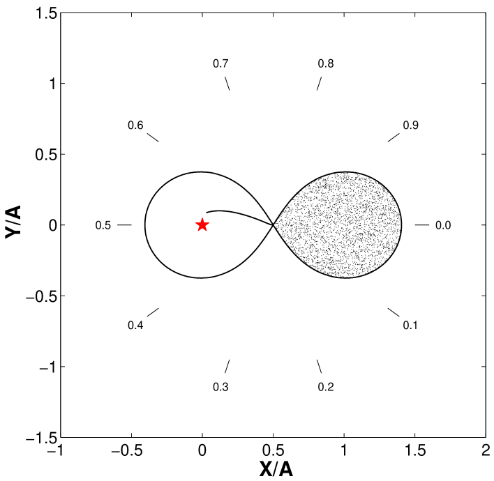
Figure 1: The adopted coordinate system with phase angles of observer in a binary system. The $x$ and $y$ coordinates are expressed in terms of the separation $A$. The red asterisk is the accretor. The donor-star is shadowed. The critical Roche lobe and ballistic trajectory of a particle moving from $L_{1}$ are shown by a solid lines. Orbital rotation of the binary is counter-clockwise.

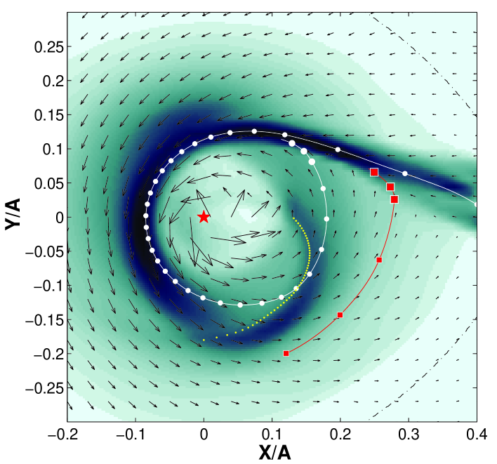
Figure 2: The distribution of density over the equatorial plane. The $x$ and $y$ coordinates are expressed in terms of the separation $A$. Arrows are the velocity vectors in observer’s frame. The red asterisk is the accretor. The dashed-dotted line is Roche equipotential passing through $L_{1}$. The yellow dotted line is the tidally induced spiral shock. Gas dynamical trajectory of a particle moving from $L_{1}$ to accretor is shown by a white line with circles. Another gas dynamical trajectory is shown by a red line with squares (see also Fig. 6).

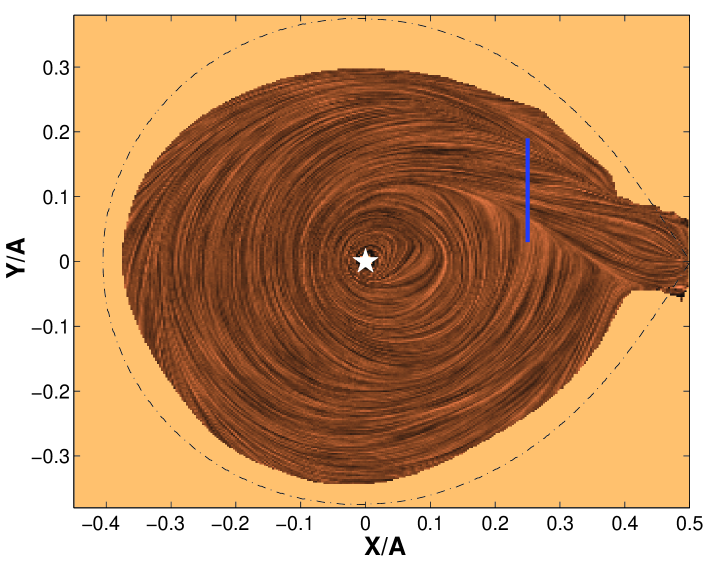
Figure 3: The texture of flow the equatorial plane (in corotation frame), i.e. visualization of velocity vectors field using Line Integral Convolution Method [20]. The white asterisk is an accretor. See Fig. 4 for the explanation of a blue line.

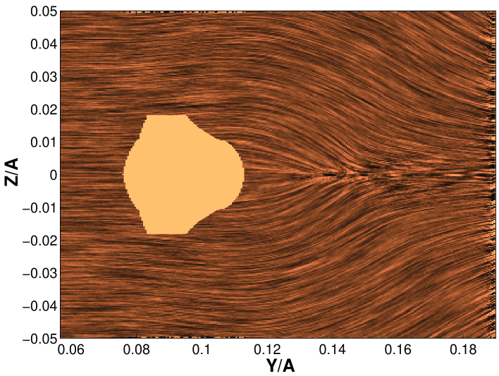
Figure 4: The texture of flow the $YZ$ slice along a blue line in Fig. 3. Empty region corresponds to cross-section of the stream from $L_{1}$.

3D gas dynamical simulations: the model and results

The full description of the used 3D gas dynamical model can be found in [10]. Here we pay attention only to the main features of the model.

Let us consider the semidetached binary system with mass of accretor $M_{1}$, mass of donor-star $M_{2}$, separation $A$, and velocity of orbital rotation $\Omega$. These parameters are connected by third Kepler’s low $A^{3}\Omega^{2}=G(M_{1}+M_{2})$. To describe the gas flow in this binary system we used the 3D system of Euler equations. The calculations were carried out in the non-inertial Cartesian coordinate system rotating with the binary system. To close the system of equations, we used the equation of state of ideal gas $P=(\gamma-1)\rho\varepsilon$, where $\gamma$ is the ratio of heat capacities. To mimic the system with radiative losses, we accept in the model the value of adiabatic index close to unit: $\gamma=1.01$, that corresponds to the case close to the isothermal one [11, 12].

To obtain numerical solution of the system of equations we used the Roe–Osher TVD scheme of a high approximation order [13, 14] with Einfeldt modification [15]. The original system of equations was written in a dimensionless form. To do this, the spatial variables were normalized to the distance between the components $A$, the time variables were normalized to the reciprocal angular velocity of the system ${\Omega}^{-1}$, and the density was normalized to its value in the inner Lagrangian point $L_{1}$. We adopted the computational domain as a parallepipedon $[-\hbox{$\,{}^{1}\!/_{2}$}A\ldots\hbox{$\,{}^{1}\!/_{2}$}A]\times[-\hbox{$\,{}^{1}\!/_{2}$}A\ldots\hbox{$\,{}^{1}\!/_{2}$}A]\times[0\ldots\hbox{$\,{}^{1}\!/_{4}$}A]$ (due to the symmetry of the problem calculations were conducted only in the top half-space). A sphere with a radius of $\hbox{$\,{}^{1}\!/_{100}$}A$ representing the accretor was cut out of the calculation domain. The boundary conditions were taken as ‘free outflow’ on the accretor star and on the outer edges of computational domain. In gridpoint corresponding to $L_{1}$ we injected the matter with parameters $\rho=\rho(L_{1})$, $V_{x}=c(L_{1})$, $V_{y}=V_{z}=0$, where $c(L_{1})$ is a gas speed of sound in $L_{1}$ point. As the initial conditions we used rarefied gas with the following parameters $\rho_{0}=10^{-5}\cdot\rho(L_{1})$, $P_{0}=10^{-4}\rho(L_{1})c^{2}(L_{1})/\gamma$, ${{\mathchoice{\hbox{$\displaystyle V$}}{\hbox{$\textstyle V$}}{\hbox{$\scriptstyle V$}}{\hbox{$\scriptscriptstyle V$}}}}_{0}=0$.

Analysis of considered problem shows that the gas dynamical solution is defined by three dimensionless parameters [16–18]: mass ratio $q=M_{2}/M_{1}$, Lubow-Shu parameter $\epsilon=c(L_{1})/A\Omega$ [16], and adiabatic index $\gamma$. The value of adiabatic index was discussed above and we used the value $\gamma=1.01$. Analysis of our previous results [17, 18] shows that the main characteristic features of 3D gas dynamical flow structure are qualitatively the same in wide range of parameters $q$ and $\epsilon$. Therefore for model simulation we chose them as follows: $q=1$, $\epsilon=\hbox{$\,{}^{1}\!/_{10}$}$.

The results of calculations will be presented in coordinate system (see Fig. 1) which is widely used in Doppler mapping. The origin of coordinates is located in the center of the accretor, ‘$x$’-axis is directed along the line connecting the centers of stars, from accretor to the mass-losing component, ‘$z$’-axis is directed along the axis of rotation, and ‘$y$’-axis is determined so that we obtain a right-hand coordinate system (i.e. ‘$y$’-axis points in the direction of orbital movement of the donor-star). In Fig. 1 we put digits showing the phase angles of the observer in binary system. We also show a critical Roche lobe with shadowed donor-star and ballistic trajectory of a particle moving from $L_{1}$ point to accretor.

The morphology of gaseous flows in considered binary system can be evaluated from Figs 2, 3 and 4. In Fig. 2 the distribution of density over the equatorial plane and velocity vectors are presented. In this Figure we also put a gas dynamical trajectory of a particle moving from $L_{1}$ to accretor (a white line with circles) and a gas dynamical trajectory passing through the shock wave along the stream edge (a red line with squares, see also Fig. 6). In Fig. 3 we present the so called texture figure in equatorial plane which is visualization of velocity vectors field using Line Integral Convolution Method [20]. In Fig. 4 the similar texture is presented for $YZ$ slice along a blue line in Fig. 3. Empty region in Fig. 4 corresponds to cross-section of the stream.

Analysis of presented results as well as our previous studies [21, 22] show the significant influence of rarefied gas of circumbinary envelope on the flow patterns in semidetached binaries. The gas of circumbinary envelope interacts with the stream of matter and deflects it. This leads, in particular, to the shock-free (tangential) interaction between the stream and the outer edge of forming accretion disc, and, as the consequence, to the absence of ‘hot spot’ in the disc. At the same time it is seen, that the interaction of the gas of circumbinary envelope with the stream results in the formation of an extended shock wave located along the stream edge (‘hot line’). From Figs 2 and 3 it also seen that spiral shock tidally induced by donor-star appears (dotted line in Fig. 2). Appearance of tidally induced two-armed spiral shock was discovered by Matsuda [19, 23, 24]. Here we see only one-armed spiral shock. In the place where the second arm should be we see the strong gas dynamical interaction of circumbinary envelope with the stream causing the formation of rather intensive shock along the outer edge of the stream. This gas dynamically induced shock probably prevents the formation of second arm of tidally induced spiral shock.

An analysis of the flow structure in $YZ$ plane (Fig. 4) shows that a part of the circumstellar envelope interacts with the (denser) original gas stream and is deflected away from the orbital plane. This naturally leads to the formation of ‘halo’. Following to [10], one can define ‘halo’ as that matter which: i) encircles the accretor being gravitationally captured; ii) does not belong to the accretion disc; iii) interacts with the stream (collides with it and/or overflows it); iv) after the interaction either becomes a part of the accretion disc or leaves the system.

Described gas dynamical features of flow structure are good candidates to be observed using Doppler mapping technique.

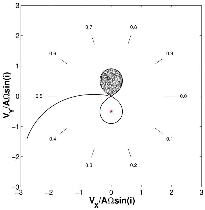
Figure 5: The adopted velocity coordinate system with phase angles of observer in a binary system. The critical Roche lobe and ballistic trajectory of a particle moving from $L_{1}$ point to accretor are shown by a solid line. The red asterisk is the accretor. The donor-star is shadowed.

Synthetic Doppler maps: methodics

The Doppler maps show the distribution of luminosity in the velocity space. Each point of flow has a three-dimensional vector of velocity ${{\mathchoice{\hbox{$\displaystyle U$}}{\hbox{$\textstyle U$}}{\hbox{$\scriptstyle U$}}{\hbox{$\scriptscriptstyle U$}}}}=(U_{x},U_{y},U_{z})$ in observer’s (inertial) frame. In the case when observer is located in the orbital plane of the binary the Doppler map’s coordinate $(V_{x},V_{y})$ will coincide with $U_{x}$ and $U_{y}$. To define these coordinates for the case of inclined system we have to find a projection of vector $\textstyle U$ on the plane constituted by vectors $\textstyle n$ and ${{\mathchoice{\hbox{$\displaystyle n$}}{\hbox{$\textstyle n$}}{\hbox{$\scriptstyle n$}}{\hbox{$\scriptscriptstyle n$}}}}\times{{\mathchoice{\hbox{$\displaystyle\Omega$}}{\hbox{$\textstyle\Omega$}}{\hbox{$\scriptstyle\Omega$}}{\hbox{$\scriptscriptstyle\Omega$}}}}$, where $\textstyle n$ is a direction from the observer to binary.

The line emissivity in the velocity space can be written as:

$$I(V_{x},V_{y})\sim\int\limits_{\cal O}\int\limits_{U_{x}}\int\limits_{U_{y}}I(x,y,z)\delta(U_{x}(x,y,z)\sin i+U_{z}(x,y,z)\cos i-V_{x})$$

$$\qquad\qquad\qquad\qquad\delta(U_{y}(x,y,z)\sin i+U_{z}(x,y,z)\cos i-V_{y})d{\cal O}dU_{x}dU_{y}\,,$$

where $d{\cal O}=dxdydz$, $i$ – inclination angle. Usually $U_{z}\ll U_{x},U_{y}$ in the most dense parts of the flow therefore we can neglect the third component of velocity $U_{z}$. This assumption allows us to take off ‘$\sin i$’ beyond the integral and to simplify the expression. Using $V_{x}/\sin i$ and $V_{y}/\sin i$ as coordinates for Doppler map will hide the dependency on the inclination angle.

The adopted dimensionless coordinate system for Doppler maps is shown in Fig. 5. We also put in Fig. 5 digits (the same as in Fig. 1) showing the phase angles of observer in binary system. The transformation of the donor-star from spatial to velocity coordinate system is very simple as it is fixed in the corotating frame. Every point $\textstyle r$ fixed in the binary frame has a velocity ${{\mathchoice{\hbox{$\displaystyle\Omega$}}{\hbox{$\textstyle\Omega$}}{\hbox{$\scriptstyle\Omega$}}{\hbox{$\scriptscriptstyle\Omega$}}}}\times{{\mathchoice{\hbox{$\displaystyle r$}}{\hbox{$\textstyle r$}}{\hbox{$\scriptstyle r$}}{\hbox{$\scriptscriptstyle r$}}}}$ in corotation frame. This is linear in the perpendicular distance from the rotation axis and therefore the shape of the donor-star projected on the orbital plane is preserved (see Fig. 5). Since the velocity of each point of donor-star is perpendicular to the radius vector, all points of donor-star are rotated by 90^∘ counter-clockwise between the spatial (see Fig. 1) and velocity coordinate diagrams [1].

Figure 5 depicts in velocity coordinates a critical Roche lobe with shadowed donor-star and ballistic trajectory of a particle moving from $L_{1}$ to accretor. On the velocity plane the accretor has coordinates (0,$K_{1}$), where $K_{1}=-A\Omega M_{2}/(M_{1}+M_{2})$ or in dimensionless form (for adopted value of $q=1$) $K_{1}=-\hbox{$\,{}^{1}\!/_{2}$}$.

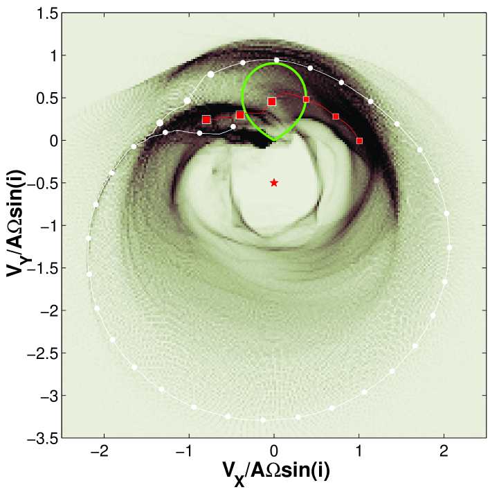
Figure 6: Synthetic Doppler map for $I=\rho$. The secondary Roche lobe (a bold green line) and the accretor (a red asterisk) are also shown. The white line with circles and red line with squares show gas dynamical trajectories in the velocity coordinates (see Fig. 2).

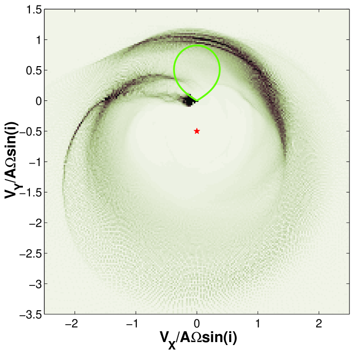
Figure 7: Synthetic Doppler map for $I=\rho^{2}T^{1/2}$.

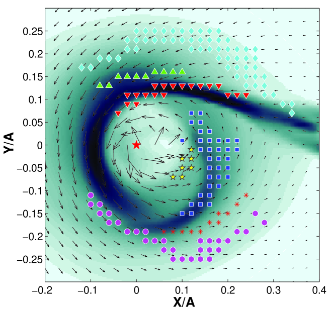
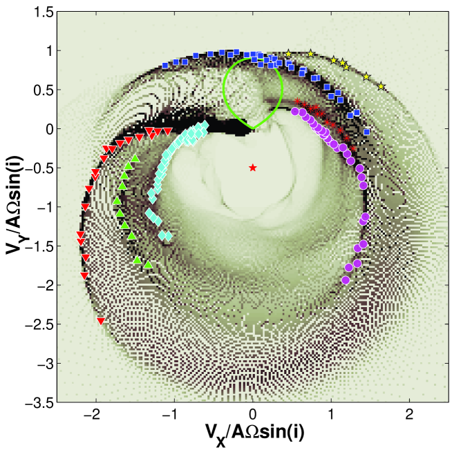
Figure 8: (Upper panel) Density and velocity distribution in equatorial plane with marked sites. (Lower panel) Synthetic Doppler map corresponding to the equatorial plane with the same marks.

Synthetic Doppler maps: analysis

As it was mentioned earlier we used both $I=\rho$ and $I=\rho^{2}T^{1/2}$ to build synthetic Doppler maps. The synthetic Doppler map calculated with $I=\rho$ is presented in Fig. 6. This map shows the intensity integrated over the $z$-coordinate, i.e. taking into account all $z$-layers of computational grid. Figure 7 presents the Doppler map corresponding to $I=\rho^{2}T^{1/2}$. The comparison of results presented in Figs 6 and 7 shows that all characteristic features are the same for different prescriptions of $I$, therefore for further analysis we will use results for $I=\rho$.

For the sake of comparison we have marked different features of flow structure and put these marks both in spatial and on velocity coordinates. Let us consider results presented in Figs 2 and 6. As it follows from these figures stream from $L_{1}$ (first part of curve marked by white line with circles) transforms to a spiral arm in the 2-nd and 3-d quadrants of the Doppler map. Shock wave caused by interaction of circumbinary envelope with the stream is located along the stream edge in spatial coordinates. Three last points (marked by larger symbols) of curves with circles and squares in Fig. 2 are the examples of two flowlines passing through the shock. The position of this shock on Doppler map is an spiral arm starting approximately from the center of donor-star in the direction of negative $V_{x}$. This arm lies above the arm caused by stream from $L_{1}$.

To analyze other features we have marked the corresponding sites both in spatial and velocity coordinates (see Fig. 8a,b). This comparison is a straightforward problem since we simply choose from all sites of gas dynamical flow structure those that fall in specific places on the Doppler map and mark them. It is seen that tidally induced spiral shock (dashed line in Fig. 2) or more precisely the dense post-shock zone (blue squares in Fig. 8a) produces bright arm in the first quadrant of Doppler map. It is important to note that gas of circumbinary envelope overflowing the stream (cyan diamonds and green up triangles) significantly increase the luminosity of the zone of Doppler map located below the zone corresponding to the stream. Analysis of other features can be conducted by comparison of Figs 8a and 8b as well (magenta circles, yellow stars and red asterisks).

Doppler maps: observations

Doppler tomography of binaries is widely and actively used now. Since pioneer work by Marsh and Horne [1] a lot of Doppler map observations were made (see, e.g., [25–28]). Just to give to reader the idea on observable Doppler maps we present here in Fig. 9 two Doppler maps of HeII $\lambda~{}4686$Å  for IP Peg obtained by Morales-Rueda, Marsh and Billington [25].

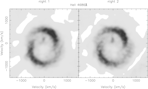
Figure 9: Doppler maps of HeII $\lambda~{}4686$Å  for IP Peg [25]. This figure is reproduced under the kind permission by L.Morales-Rueda.

Conclusions

Three-dimensional gas dynamical simulations of flow structure in semidetached binaries allow to build synthetic Doppler maps. In turn it gives a possibility to identify main features of the flow on the Doppler map without solution of ill-posed inverse problem. Comparison of synthetic tomograms with observations makes possible both to refine the gas dynamical model and to interpret the observational data.

References

- [1] Marsh T.R., and Horne K., MNRAS 235, 269 (1988).
- [2] Narayan R., and Nityananda R., Ann. Rev. Astron. Astrophys. 24, 127 (1986).
- [3] Robinson E.L., Marsh T.R., and Smak J., in Accretion Disks in Compact Stellar Systems, ed. J.C.Wheeler, World Sci. Publ., Singapore, 1993, p. 75.
- [4] Spruit H.C., preprint astro-ph/9806141 (1998).
- [5] Frieden B.R., in Picture Processing and Digital Filtering, ed. T.S.Huang, Springer-Verlag, Heidelberg, 1979, p. 177.
- [6] Horne K., and Marsh T.R., MNRAS 218, 761 (1986).
- [7] Richards M.T., and Ratliff M.A., ApJ 493, 326 (1998).
- [8] Ferland C.J., PASP 92, 596 (1980).
- [9] Kaitchuck R.H., Schlegel E.M., Honeycutt R.K., Horne K., Marsh T.R., White J.C.,II, and Mansperger C.S., ApJS 93, 519 (1994).
- [10] Bisikalo D.V., Boyarchuk A.A., Kuznetsov O.A., and Chechetkin V.M., AZh 77, 31 (2000) (Astron. Rep. 44, 26, astro-ph/9907087).
- [11] Sawada K., Matsuda T., and Hachisu I., MNRAS 219, 75 (1986).
- [12] Bisikalo D.V., Boyarchuk A.A., Kuznetsov O.A., Popov Yu.P., and Chechetkin V.M., AZh 72, 367 (1995) (Astron. Rep. 39, 325).
- [13] Roe P.L., Ann. Rev. Fluid Mech. 18, 337 (1986).
- [14] Chakravarthy S., and Osher S., AIAA Pap. N 85–0363 (1985)
- [15] Einfeldt B., SIAM J. Numer. Anal. 25, 294 (1988).
- [16] Lubow S.H., and Shu F.H., ApJ 198, 383 (1975).
- [17] Bisikalo D.V., Boyarchuk A.A., Kuznetsov O.A., and Chechetkin V.M., AZh 75, 706 (1998) (Astron. Rep. 42, 229, preprint astro-ph/9812484).
- [18] Bisikalo D.V., Boyarchuk A.A., Chechetkin V.M., Kuznetsov O.A., and Molteni D., AZh 76, 905 (1999) (Astron. Rep. 43, 797, preprint astro-ph/9907084).
- [19] Sawada K., Matsuda T., Inoue M., and Hachisu I., MNRAS 224, 307 (1987).
- [20] Cabral B., and Leedom C., in SIGGRAPH 93 Conference Proceedings, 1993, p. 263.
- [21] Bisikalo D.V., Boyarchuk A.A., Kuznetsov O.A., and Chechetkin V.M., AZh 74, 880 (1997) (Astron. Rep. 41, 786, preprint astro-ph/9802004).
- [22] Bisikalo D.V., Boyarchuk A.A., Chechetkin V.M., Kuznetsov O.A., and Molteni D., MNRAS 300, 39 (1998).
- [23] Sawada K., Matsuda T., and Hachisu I., MNRAS 219, 75 (1986).
- [24] Sawada K., Matsuda T., and Hachisu I., MNRAS 221, 679 (1986).
- [25] Morales-Rueda L., Marsh T.R., and Billington I., MNRAS 313, 454 (2000).
- [26] Steeghs D., Harlaftis E.T., and Horne K., MNRAS 290, L28 (1997).
- [27] Harlaftis E.T., Steeghs D., Horne K., Martín E., and Magazzú A., MNRAS 306, 348 (1999).
- [28] Baptista R., Harlaftis E.T., and Steeghs D., MNRAS 314, 727 (2000).