The Cosmic Background Radiation circa $\nu$2K

Abstract

We describe the implications of cosmic microwave background (CMB) observations and galaxy and cluster surveys of large scale structure (LSS) for theories of cosmic structure formation, especially emphasizing the recent Boomerang and Maxima CMB balloon experiments. The inflation-based cosmic structure formation paradigm we have been operating with for two decades has never been in better shape. Here we primarily focus on a simplified inflation parameter set, $\{\omega_{b},\omega_{cdm},\Omega_{tot},\Omega_{\Lambda},n_{s},\tau_{C},\sigma_{8}\}$. Combining all of the current CMB+LSS data points to the remarkable conclusion that the local Hubble patch we can access has little mean curvature ($\Omega_{tot}=1.08\pm 0.06$) and the initial fluctuations were nearly scale invariant ($n_{s}=1.03\pm 0.08$), both predictions of (non-baroque) inflation theory. The baryon density is found to be slightly larger than that preferred by independent Big Bang Nucleosynthesis estimates ($\omega_{b}\equiv\Omega_{b}{\rm h}^{2}=0.030\pm 0.005$ cf. $0.019\pm 0.002$). The CDM density is in the expected range ($\omega_{cdm}=0.17\pm 0.02$). Even stranger is the CMB+LSS evidence that the density of the universe is dominated by unclustered energy akin to the cosmological constant ($\Omega_{\Lambda}=0.66\pm 0.06$), at the same level as that inferred from high redshift supernova observations. We also sketch the CMB+LSS implications for massive neutrinos.

1 CMB Anisotropies & Distortions

1.1 What Was Revealed in 1999/2000

As we penetrate the CMB, we go from a nearly perfect blackbody of $2.725\pm 0.002\,K$ [1], to a $3.372\pm 0.007\,mK$ dipole pattern associated with the 300 ${\rm~{}km~{}s^{-1}}$ flow of the earth in the CMB, to the now familiar motley pattern of anisotropies associated with $2\mathrel{\hbox to0.0pt{\lower 3.0pt\hbox{$-$}\hss}\raise 2.0pt\hbox{$\mathchar 316\relax$}}\ell\mathrel{\hbox to0.0pt{\lower 3.0pt\hbox{$\mathchar 536\relax$}\hss}\raise 2.0pt\hbox{$\mathchar 316\relax$}}20$ multipoles at the $30\mu K$ level revealed by COBE at $7^{\circ}$ resolution, then at higher $\ell$ in some 19 other experiments (though most with many fewer resolution elements than the 600 or so for COBE). The picture was dramatically improved this year, as results were announced first in summer 99 from the ground-based TOCO experiment in Chile [2], then in November 1999 from the North American balloon test flight of Boomerang [3], then in April 2000 from the first CMB long duration balloon (LDB) flight, of Boomerang [4], followed in May 2000 from the night flight of Maxima [5]. Boomerang’s best resolution was $10^{\prime}$, about 40 times better than that of COBE, with tens of thousands of resolution elements. Maxima had a similar resolution but covered an order of magnitude less sky. Both experiments were designed to reveal the primary anisotropies of the CMB, those which can be calculated using linear perturbation theory. What we see in Fig. 1 are two images of soundwave patterns that existed about 300,000 years after the Big Bang, when the photons were freed from the plasma. The visually evident structure on degree scales is even more apparent in the power spectra of the Fourier transform of the maps (Fig. 2), which show a dominant (first acoustic) peak, a less prominent (or non-existent) second one, and the hint of a third one from Maxima. In the following, we describe the implications of these results for cosmology. Space constraints preclude adequate referencing here, but these are given in [6, 7, 8].

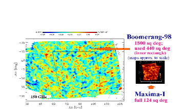
Figure 1: The Boomerang 150A GHz bolometer map (one out of 16) is shown. Of the entire 1800 square degrees covered (not all of which is shown), only the interior 440 sq. degs. within the central rectangle were used in our analysis, i.e., in all less than 5% of the data. The 124 square degree Maxima-I map, drawn to scale, is also shown. Bandpowers derived from these maps and their noise correlation matrices (Figure 2) were used to derive the parameters given in Table 1.

We are only at the beginning of the high precision CMB era. HEMT-based interferometers are already in place taking data: the VSA (Very Small Array) in Tenerife, the CBI (Cosmic Background Imager) in Chile, DASI (Degree Angular Scale Interferometer) at the South Pole, where the bolometer-based single dish ACBAR experiment will operate this year. Other LDBs will be flying within the next few years: Arkeops, Tophat, Beast/Boost; and in 2001, Boomerang will fly again, this time concentrating on polarization. As well, MAXIMA will fly as the polarization-targeting MAXIPOL. In April 2001, NASA will launch the all-sky HEMT-based MAP satellite, with $12^{\prime}$ resolution. Further downstream in 2007, ESA will launch the bolometer+HEMT-based Planck satellite, with $5^{\prime}$ resolution.

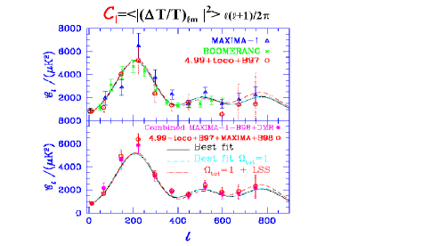
Figure 2: The ${\cal C}_{\ell}$ (defined in terms of CMB temperature anisotropy multipoles, $(\Delta T/T)_{\ell m}$, as indicated) grouped in bandpowers for prior-CMB experiments, including TOCO and the North American Boomerang test flight, (squares) are contrasted with the Boomerang-98 LDB (crosses) and Maxima-I (triangles) results in the upper panel. The lower panel shows the optimally combined power spectra of Boomerang+Maxima+DMR (squares) and contrasts it with that for Boomerang+Maxima+prior-CMB (circles), showing that including the prior experiments does not make a large difference to the results. Best-fit models for arbitrary $\Omega_{tot}$ and for the restriction to the flat case are shown in both panels.

1.2 Primary & Secondary Processes

As we peer back in time, we reach a fuzzy wall at redshift $z\sim 1100$, the photon decoupling ”surface”, through which the Universe passed from optically thick to thin to Thomson scattering over a physical distance $\sim 10{\rm~{}kpc}$, i.e., $\sim 10{\rm~{}Mpc}$ comoving. Prior to this, acoustic wave patterns in the tightly-coupled photon-baryon fluid on scales below the ”sound crossing distance” at decoupling, $\mathrel{\hbox to0.0pt{\lower 3.0pt\hbox{$\mathchar 536\relax$}\hss}\raise 2.0pt\hbox{$\mathchar 316\relax$}}100{\rm~{}kpc}$ physical, $\mathrel{\hbox to0.0pt{\lower 3.0pt\hbox{$\mathchar 536\relax$}\hss}\raise 2.0pt\hbox{$\mathchar 316\relax$}}100{\rm~{}Mpc}$ comoving, were viscously damped, strongly so on scales below the $\sim 10{\rm~{}kpc}$ thickness over which decoupling occurred. After, photons freely-streamed along geodesics to us, mapping (through the angular diameter distance relation) the post-decoupling spatial structures in the temperature to the angular patterns we observe now as the primary CMB anisotropies. The maps are images projected through the fuzzy decoupling surface of the acoustic waves (photon bunching), the electron flow (Doppler effect) and the gravitational potential peaks and troughs (”naive” Sachs-Wolfe effect) back then. Free-streaming along our (linearly perturbed) past light cone leaves the pattern largely unaffected, except that temporal evolution in the gravitational potential wells as the photons propagate through them leaves a further $\Delta T$ imprint, called the integrated Sachs-Wolfe effect. Intense theoretical work over three decades has put accurate calculations of this linear cosmological radiative transfer on a firm footing, and there is a speedy, publicly available and widely used code for evaluation of anisotropies in a wide variety of cosmological scenarios, “CMBfast” [9].

Secondary anisotropies associated with nonlinear effects also leave an imprint. The photons were weakly-lensed by intervening mass, were Thompson-scattered by the flowing gas once it became ”reionized” at $z\sim 20$, and were occasionally Compton-upscattered, with mean fractional energy shifts $4T_{gas}/m_{e}c^{2}$, by nonlinear hot gas (thermal Sunyaev-Zeldovich or Compton cooling effect); the flowing cluster induces a further kinetic SZ effect. Of these secondary processes, all have the same spectral signature of a perturbed blackbody, with a $\lambda$-independent thermodynamic temperature perturbation, $\Delta T(\lambda,{\hat{q}})$ — except for the thermal SZ effect.

The SZ spectral distortion is related to the Compton $y$ parameter, which is proportional to the line of sight integral of the electron pressure: $\Delta T$ is negative, $-2y$, on the Rayleigh-Jeans side and positive on the Wien side, $(E_{\gamma}/T_{cmb})y$, passing through zero at $1378\mu{\rm m}$ or 218 GHz. The COBE FIRAS experiment limits the energy injection that leads to the thermal SZ pattern to be ${\delta E_{Compton\ cool}/E_{cmb}}=4y<6.0\times 10^{-5}$ (95% CL) [1]. It is routine now to see the (concentrated) fluctuations in $y$ from clusters, though the sky-average $y$ is predicted to be $\mathrel{\hbox to0.0pt{\lower 3.0pt\hbox{$\mathchar 536\relax$}\hss}\raise 2.0pt\hbox{$\mathchar 316\relax$}}10^{-5}$. SZ anisotropies have been probed by single dishes, the OVRO and BIMA mm arrays, and the Ryle interferometer. A number of HEMT-based interferometers being built are more ambitious: AMI (Britain), the JCA (Chicago), AMIBA (Taiwan), MINT (Princeton). As well, other kinds of bolometer-based experiments will be used to probe the SZ effect, including the CSO (Caltech submm observatory) with BOLOCAM on Mauna Kea, ACBAR at the South Pole, the LMT (large mm telescope) in Mexico, and the LDB BLAST.

A secondary anisotropy not associated with the CMB photons is stellar and accretion disk radiation reprocessed by dust into the infrared and redshifted into the submm, leading to a Wien tail distortion of the CMB blackbody. This has been found in the COBE FIRAS and shorter wavelength DIRBE data, with energy at a level about twice that in optical light. Anisotropies from dust emission from high redshift galaxies are being targeted by the JCMT with the SCUBA bolometer array, the CSO (soon with BOLOCAM), the OVRO mm interferometer, the SMA (submm array) on Mauna Kea, the LMT, the ambitious US/ESO ALMA array in Chile, the LDB BLAST, and ESA’s FIRST satellite. About $50\%$ of the submm background has so far been identified with sources that SCUBA has found.

${\cal C}_{\ell}$’s from nonlinearities in the gas at high redshift are concentrated at high $\ell$, but for most viable models are expected to be a small contaminant. Similarly, Thomson scattering from gas in moving clusters also has a small effect on ${\cal C}_{\ell}$ (although it should be measurable in individual clusters, e.g., with BOLOCAM and with Planck). The effect of lensing is to smooth slightly the acoustic peaks and troughs of Fig. 2 and induce small scale non-Gaussian effects.

1.3 Boomerang & Maxima

Boomerang carried a 1.2m telescope with 16 bolometers cooled to 0.3K in the focal plane aloft from McMurdo Bay in Antarctica in late December 1998, circled the Pole for 10.6 days and landed just 50 km from the launch site, only slightly damaged. In [4], maps at 90, 150 and 220 GHz showed the same spatial features and the intensities were shown to fall precisely on the CMB blackbody curve. The fourth frequency channel at 400 GHz is dust-dominated. Fig. 1 shows the 150 GHz map derived using only one of the 16 bolometers. Although Boomerang altogether probed 1800 square degrees, only the region in the rectangle covering 440 square degrees was used in the analysis described in [7, 8] and this paper. Fig. 1 also shows the 124 square degree region of the sky (in the Northern Hemisphere) that Maxima-1 probed. Though Maxima was not an LDB, it did so well because its bolometers were cooled even more than Boomerang’s, leading to higher sensitivity per unit observing time; further, all frequency channels were used in creating its map.

Analyzing Boomerang and other experiments involves a pipeline that takes (1) the timestream in each of the bolometer channels coming from the balloon plus information on where it is pointing and turns it into (2) spatial maps for each frequency characterized by average temperature fluctuation values in each pixel (Fig. 1) and a pixel-pixel correlation matrix characterizing the noise, from which various statistical quantities are derived, in particular (3) the temperature power spectrum as a function of multipole (Fig. 2), grouped into bands, and two band-band error matrices which together determine the full likelihood distribution of the bandpowers [10]. Fundamental to the first step is the extraction of the sky signal from the noise, using the only information we have, the pointing matrix mapping a bit in time onto a pixel position on the sky.

There is generally another step in between (2) and (3), namely separating the multifrequency spatial maps into the physical components on the sky: the primary CMB, the thermal and kinematic Sunyaev-Zeldovich effects, the dust, synchrotron and bremsstrahlung Galactic signals, the extragalactic radio and submillimetre sources. The strong agreement among the Boomerang maps indicates that to first order we can ignore this step, but it has to be taken into account as the precision increases. The Fig. 2 map is consistent with a Gaussian distribution, thus fully characterized by just the power spectrum. Higher order (concentration) statistics (3,4-point functions, etc.) tell us of non-Gaussian aspects, necessarily expected from the Galactic foreground and extragalactic source signals, but possible even in the early Universe fluctuations. For example, though non-Gaussianity occurs only in the more baroque inflation models of quantum noise, it is a necessary outcome of defect-driven models of structure formation. (Peaks compatible with Fig. 2 do not appear in non-baroque defect models, which now appear unlikely.)

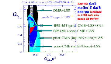
Figure 3: 2-sigma likelihood contours for the dark matter density and dark energy density (assuming $w_{Q}=-1$, i.e., a cosmological constant) are shown when progressively more CMB data are added to the LSS data. The smallest 2-sigma region shows what happens when SNIa data is added to Boomerang+Maxima+prior-CMB+LSS. In all cases, the weak-H+age prior probability is adopted. Other variables have been marginalized, as in Table 1.

1.4 Parameters of Structure Formation

For this paper, we adopt the restricted set of 7 cosmological parameters used in [7, 8]. Among these, we have 2 characterizing the early universe primordial power spectrum of gravitational potential fluctuations $\Phi$, one giving the overall power spectrum amplitude ${\cal P}_{\Phi}(k_{n})$, and one defining the shape, a spectral tilt $n_{s}(k_{n})\equiv 1+d\ln{\cal P}_{\Phi}/d\ln k$, at some (comoving) normalization wavenumber $k_{n}$. We really need another 2, ${\cal P}_{GW}(k_{n})$ and $n_{t}(k_{n})$, associated with the gravitational wave component. In inflation, the amplitude ratio is related to $n_{t}$ to lowest order, with ${\cal O}(n_{s}-n_{t})$ corrections at higher order, e.g., [6]. There are also useful limiting cases for the $n_{s}-n_{t}$ relation. However, as one allows the baroqueness of the inflation models to increase, one can entertain essentially any power spectrum (fully $k$-dependent $n_{s}(k)$ and $n_{t}(k)$) if one is artful enough in designing inflaton potential surfaces. As well, one can have more types of modes present, e.g., scalar isocurvature modes (${\cal P}_{is}(k_{n}),n_{is}(k)$) in addition to, or in place of, the scalar curvature modes (${\cal P}_{\Phi}(k_{n}),n_{s}(k)$). However, our philosophy is consider minimal models first, then see how progressive relaxation of the constraints on the inflation models, at the expense of increasing baroqueness, causes the parameter errors to open up. For example, with COBE-DMR and Boomerang, we can probe the GW contribution, but the data are not powerful enough to determine much. Planck can in principle probe the gravity wave contribution reasonably well.

We use another 2 parameters to characterize the transport of the radiation through the era of photon decoupling, which is sensitive to the physical density of the various species of particles present then, $\omega_{j}\equiv\Omega_{j}{\rm h}^{2}$. We really need 4: $\omega_{b}$ for the baryons, $\omega_{cdm}$ for the cold dark matter, $\omega_{hdm}$ for the hot dark matter (massive but light neutrinos), and $\omega_{er}$ for the relativistic particles present at that time (photons, very light neutrinos, and possibly weakly interacting products of late time particle decays). For simplicity, though, we restrict ourselves to the conventional 3 species of relativistic neutrinos plus photons, with $\omega_{er}$ therefore fixed by the CMB temperature and the relationship between the neutrino and photon temperatures determined by the extra photon entropy accompanying $e^{+}e^{-}$ annihilation. Rather than be exhaustive when the data does not warrant it, the effect of massive neutrinos is shown in Fig. 4 for a few values of $\omega_{hdm}/\omega_{m}$, where $\omega_{m}\equiv\omega_{hdm}+\omega_{cdm}+\omega_{b}$.

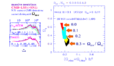
Figure 4: 2-sigma likelihood contours in the $(\omega_{cdm}+\omega_{hdm})$—$\Omega_{\Lambda}$ plane are shown as the fraction of matter in massive neutrinos is increased from 0 up to 0.3, for Boomerang+Maxima+prior-CMB+LSS when the weak-H+age + $\Omega_{tot}=1$ prior probability is adopted. The age restriction used here, $11<$ age $<16$ Gyr, is slightly stronger than the $>10$ Gyr weak-age prior adopted for the Table 1 limits. The CMB data alone cannot now discriminate among the cases — the left plot contrasts the large ${\cal C}_{\ell}$ variation as $n_{s}$ is varied over the tiny one as $\Omega_{hdm}$ is varied from 0 to 0.95. When LSS is added, the contours shift in the expected direction, with more (cold+hot) dark matter preferred, at the expense of less dark energy. Nonetheless, significant dark energy is apparently required. Note that the simplest interpretation of the superKamiokande data on atmospheric $\nu_{\mu}$ is that $\Omega_{\nu_{\tau}}\sim 0.001$, about the energy density of stars in the universe, which implies a cosmologically negligible effect. Degeneracy between e.g., $\nu_{\mu}$ and $\nu_{\tau}$ could lead to the cosmologically very interesting $\Omega_{m\nu}\equiv\Omega_{hdm}\sim 0.1$, although the coincidence of closely related energy densities for baryons, CDM, HDM and dark energy required would be amazing. The $\omega_{b}$ and $n_{s}$ likelihood curves are essentially independent of $\Omega_{m\nu}/\Omega_{m}$ for fixed $\Omega_{m}$.

The angular diameter distance relation adds dependence upon $(1-\Omega_{tot})$ and $\Omega_{\Lambda}$ as well as on $\Omega_{m}\equiv\omega_{m}/{\rm h}^{2}$ [12]. This defines a functional relationship between $\Omega_{tot}$ and $\Omega_{\Lambda}$, a degeneracy [11] that would be exact except for the integrated Sachs-Wolfe effect, associated with the change of $\Phi$ with time if $\Omega_{\Lambda}$ or $\Omega_{k}$ is nonzero. (If $\dot{\Phi}$ vanishes, the energy of photons coming into potential wells is the same as that coming out, and there is no net impact of the rippled light cone upon the observed $\Delta T$.)

Our 7th parameter is an astrophysical one, the Compton ”optical depth” $\tau_{C}$ from a reionization redshift $z_{reh}$ to the present. It lowers ${\cal C}_{\ell}$ by $\exp(-2\tau_{C})$ at the high $\ell$’s probed by Boomerang. For typical models of hierarchical structure formation, we expect $\tau_{C}\mathrel{\hbox to0.0pt{\lower 3.0pt\hbox{$\mathchar 536\relax$}\hss}\raise 2.0pt\hbox{$\mathchar 316\relax$}}0.2$. It is partly degenerate with $\sigma_{8}$ and cannot be determined at this precision by CMB data now.

The LSS also depends upon our parameter set: the most important combination is the wavenumber of the horizon when the energy density in relativistic particles equals the energy density in nonrelativistic particles: $k_{Heq}^{-1}\approx 5\Gamma^{-1}{\,{\rm h}^{-1}~{}\rm Mpc}$, where $\Gamma\approx\Omega_{m}{\rm h}\Omega_{er}^{-1/2}$. Instead of ${\cal P}_{\Phi}(k_{n})$ for the amplitude parameter, we often use ${\cal C}_{10}$ at $\ell=10$ for CMB only, and $\sigma_{8}^{2}$ when LSS is added; $\sigma_{8}^{2}$ is a bandpower for density fluctuations at $8{\,{\rm h}^{-1}~{}\rm Mpc}$, a scale associated with rare clusters of galaxies. When LSS is considered in this paper, it refers to constraints on $\Gamma+(n_{s}-1)/2$ and $\ln\sigma_{8}^{2}$ that are obtained by comparison with the data on galaxy clustering and cluster abundances [7].

When we allow for freedom in $\omega_{er}$, the abundance of primordial helium, tilts of tilts ($dn_{\{s,is,t\}}(k_{n})/d\ln k,...$) for 3 types of perturbations, the parameter count would be 17, and many more if we open up full theoretical freedom in spectral shapes. However, as we shall see, as of now only 3 or 4 combinations can be determined with 10% accuracy with the CMB.

Table 1: Cosmological parameter values and their 1-sigma errors are shown, determined after marginalizing over the other $6$ cosmological and $4^{+}$ experimental parameters, for B98+Maxima-I+prior-CMB and the weak prior used in [7, 8] ($0.45\mathrel{\hbox to0.0pt{\lower 3.0pt\hbox{$-$}\hss}\raise 2.0pt\hbox{$\mathchar 316\relax$}}{\rm h}\mathrel{\hbox to0.0pt{\lower 3.0pt\hbox{$-$}\hss}\raise 2.0pt\hbox{$\mathchar 316\relax$}}0.9$, age $>10$ Gyr). The LSS prior was also designed to be weak. The detections are clearly very stable if extra ”prior” probabilities for LSS and SN1 are included. (Indeed, they are stable to inclusion of stronger priors -except if the BBN-derived $0.019\pm 0.002$ is imposed [7].) Similar tables for B98+DMR are given in [7] and for B98+MAXIMA-I+DMR in [8]. If $\Omega_{tot}$ is varied, parameters derived from our basic 7 come out to be: age=$13.2\pm 1.3$ Gyr, ${\rm h}=0.70\pm 0.09$, $\Omega_{m}=0.35\pm.06$, $\Omega_{b}=0.065\pm.02$. Restriction to $\Omega_{tot}=1$ yields: age=$11.6\pm 0.4$ Gyr, ${\rm h}=0.80\pm.04$, $\Omega_{m}=0.31\pm.03$, $\Omega_{b}=0.046\pm.005$.

	cmb	+LSS	+SN1	+SN1,LSS	cmb	+LSS	+SN1	+SN1,LSS
$\Omega_{tot}$	$1.09^{+.07}_{-.07}$	$1.08^{+.06}_{-.06}$	$1.04^{+.06}_{-.05}$	$1.04^{+.05}_{-.04}$	1.0	1.0	1.0	1.0
$\Omega_{b}{\rm h}^{2}$	$.031^{+.005}_{-.005}$	$.031^{+.005}_{-.005}$	$.031^{+.005}_{-.005}$	$.031^{+.005}_{-.005}$	$.030^{+.004}_{-.004}$	$.030^{+.003}_{-.004}$	$.030^{+.004}_{-.004}$	$.030^{+.003}_{-.004}$
$\Omega_{cdm}{\rm h}^{2}$	$.17^{+.06}_{-.05}$	$.14^{+.03}_{-.02}$	$.13^{+.05}_{-.05}$	$.15^{+.03}_{-.02}$	$.19^{+.06}_{-.05}$	$.17^{+.02}_{-.02}$	$.16^{+.03}_{-.03}$	$.17^{+.01}_{-.02}$
$n_{s}$	$1.05^{+.09}_{-.08}$	$1.04^{+.09}_{-.08}$	$1.05^{+.10}_{-.09}$	$1.06^{+.08}_{-.08}$	$1.02^{+.08}_{-.07}$	$1.03^{+.08}_{-.07}$	$1.03^{+.08}_{-.07}$	$1.04^{+.07}_{-.07}$
$\Omega_{\Lambda}$	$0.48^{+.20}_{-.26}$	$0.63^{+.08}_{-.09}$	$0.72^{+.07}_{-.07}$	$0.70^{+.04}_{-.05}$	$0.58^{+.17}_{-.27}$	$0.66^{+.04}_{-.06}$	$0.71^{+.06}_{-.07}$	$0.69^{+.03}_{-.05}$

Table 1 shows there are strong detections with only the CMB data for $\Omega_{tot}$, $\omega_{b}$ and $n_{s}$ in the minimal inflation-based 7 parameter set. The ranges quoted are Bayesian 50% values and the errors are 1-sigma, obtained after projecting (marginalizing) over all other parameters. With Maxima, $\omega_{cdm}$ begins to localize, but much more so when LSS information is added. Indeed, even with just the COBE-DMR+LSS data, the 2-sigma contours shown in Fig. 3 are already localized in $\omega_{cdm}$. That $\Omega_{\Lambda}$ is not well determined is a manifestation of the $\Omega_{tot}$–$\Omega_{\Lambda}$ near-degeneracy discussed above, which is broken when LSS is added because the CMB-normalized $\sigma_{8}$ is quite different for open cf. $\Lambda$ models. Supernova at high redshift give complementary information to the CMB, but with CMB+LSS (and the inflation-based paradigm) we do not need it: the CMB+SN1 and CMB+LSS numbers are quite compatible. In our space, the Hubble parameter, ${\rm h}=(\sum_{j}(\Omega_{j}{\rm h}^{2}))^{1/2}$, and the age of the Universe, $t_{0}$, are derived functions of the $\Omega_{j}{\rm h}^{2}$: representative values are given in the Table caption.

Since this is a conference devoted to neutrinos, Fig. 4 is included to show what happens as we let the fraction of the matter in massive neutrinos vary, from 0 to 0.3. Until Planck precision, the CMB data by itself will not be able to strongly discriminate this ratio. Adding HDM does have a strong impact on the CMB-normalized $\sigma_{8}$ and the shape of the density power spectrum (effective $\Gamma$ parameter), both of which mean that adding some HDM to CDM is strongly preferred in the absence of $\Omega_{\Lambda}$. However a nonzero (though smaller) $\Omega_{\Lambda}$ is still preferred.

We can also forecast dramatically improved precision with further analysis of Boomerang and Maxima, other future LDBs, MAP and Planck. Because there are correlations among the physical variables we wish to determine, including a number of near-degeneracies beyond that for $\Omega_{tot}$–$\Omega_{\Lambda}$ [11], it is useful to disentangle them, by making combinations which diagonalize the error correlation matrix, ”parameter eigenmodes” [6, 11]. For this exercise, we will add $\omega_{hdm}$ and $n_{t}$ to our parameter mix, making 9. (The ratio ${\cal P}_{GW}(k_{n})/{\cal P}_{\Phi}(k_{n})$ is treated as fixed by $n_{t}$, a reasonably accurate inflation theory result.) The forecast for Boomerang based on the 440 sq. deg. patch with a single 150 GHz bolometer used in the published data is 3 out of 9 linear combinations should be determined to $\pm 0.1$ accuracy. This is indeed what we get in the full analysis of the Table and Boomerang+DMR only. If 4 of the 6 150 GHz channels are used and the region is doubled in size, we predict 4/9 could be determined to $\pm 0.1$ accuracy. And if the optimistic case for all the proposed LDBs is assumed, 6/9 parameter combinations could be determined to $\pm 0.1$ accuracy, 2/9 to $\pm 0.01$ accuracy. The situation improves for the satellite experiments: for MAP, we forecast 6/9 combos to $\pm 0.1$ accuracy, 3/9 to $\pm 0.01$ accuracy; for Planck, 7/9 to $\pm 0.1$ accuracy, 5/9 to $\pm 0.01$ accuracy. While we can expect systematic errors to loom as the real arbiter of accuracy, the clear forecast is for a very rosy decade of high precision CMB cosmology that we are now fully into.

References

- [1] Mather, J.C. et al., ApJ 512, 511 (1999).
- [2] Miller, A.D. et al., ApJ Lett 524, L1 (1999) TOCO.
- [3] Mauskopf, P. et al., ApJ Lett 536, L59, (2000) BOOM-97.
- [4] de Bernardis, P. et al., Nature 404, 995 (2000), astro-ph/00050087, http://www.physics.ucsb.edu/ boomerang/
- [5] Hanany, S. et al., ApJ Lett, submitted (2000), astro-ph/0005123, http://cfpa.berkeley.edu/maxima
- [6] Bond, J.R. in Cosmology and Large Scale Structure, Les Houches Session LX, eds. R. Schaeffer J. Silk, M. Spiro & J. Zinn-Justin (Elsevier Science Press, Amsterdam), pp. 469-674, (1996).
- [7] Lange, A. et al., PRD, in press (2000), astro-ph/0005004.
- [8] Jaffe, A. et al., PRL, in press (2000), astro-ph/0007333.
- [9] Seljak U. & Zaldarriaga M., ApJ, 469, 437 (1996).
- [10] Bond, J.R., Jaffe, A.H. & Knox, L., PRD 57, 2117 (1998), astro-ph/9708203; ApJ 533, 19 (2000), astro-ph/9808264.
- [11] e.g., Efstathiou, G. & Bond, J.R., Mon. Not. R. Astron. Soc. 304, 75 (1999), where many other near-degeneracies between cosmological parameters are also discussed.
- [12] The dark energy parameterized here by could have complex dynamics associated with it, e.g., if it is the energy density of a scalar field which dominates at late times (now often termed a quintessence field, , with energy - see http://feynman.princeton.edu/ steinh/ ”Quintessence? - an overview” for a pedagogical introduction). One popular phenomenology is to add one more parameter, , where and are the pressure and density of the -field. Thus and for the cosmological constant. The CMB and LSS does not currently give a useful constraint on , though SN1 apparently gives .